S T R U C T U R E L E A R N I N G r i t e s h a j o o d h a
A Ph.D. thesis submitted to the Faculty of Science, University of the Witwatersrand, in fulfillment of the requirements for the degree of Doctor of Philosophy in Computer
Science.
Doctor of Philosophy
Supervised by Dr. Benjamin Rosman
School of Computer Science and Applied Mathematics The University of the Witwatersrand
using Score-based Structure Learning,Doctor of Philosophy.
A Ph.D. thesis submitted to the Faculty of Science, University of the Witwatersrand, in fulfillment of the requirements for the degree of Doctor of Philosophy in Computer Science.
s u p e r v i s o r:
Dr. Benjamin Rosman
l o c at i o n:
January. She was8years old when she lost her mother. In1947she married Mr. Bhoodan Ajoodha and lived on56Croesus Avenue in Newclare. In1960she leased her farm in Lenasia (95Nirvana Avenue) and, together with her husband, she bought the first house in
Lenasia and had12children (6sons and6daughters),35grand-children,43
great-grand-children, and3great-great-grand-children. As one of her93descendents, I am proud to have shared some of her stories and experiences. She was the first Indian woman to
travel on board the Concorde1, crossing two international time-lines. At the age of87she lived a fruitful and memorable life, leaving behind an impressive legacy.
(a) (b) (c)
Figure1: (a) Mr. and Mrs. Ajoodha abord the Concorde; (b) Mr. and Mrs. Ajoodha at their home, the first house in Lenasia; (c) Mrs. Ajoodha celebrating my2ndBirthday.
Although partially observable stochastic processes are ubiquitous in many fields of science, little work has been devoted to discovering and analysing the means by which several such processes may interact to influence each other. In this thesis we extend probabilistic structure
learning between random variables to the context of temporal models which represent partially observable stochastic processes. Learning an influence structure and distribution
between processes can be useful for density estimation and knowledge discovery. A common approach to structure learning, in observable data, is score-based structure learning, where we search for the most suitable structure by using a scoring metric to value structural configurations relative to the data. Most popular structure scores are variations on
the likelihood score which calculates the probability of the data given a potential structure. In observable data, the decomposability of the likelihood score, which is the ability to represent the score as a sum of family scores, allows for efficient learning procedures and significant computational saving. However, in incomplete data (either by latent variables or
missing samples), the likelihood score is not decomposable and we have to perform inference to evaluate it. This forces us to use non-linear optimisation techniques to optimise
the likelihood function. Furthermore, local changes to the network can affect other parts of the network, which makes learning with incomplete data all the more difficult. We define two general types of influence scenarios: direct influence and delayed influence
which can be used to define influence around richly structured spaces; consisting of multiple processes that are interrelated in various ways. We will see that although it is possible to capture both types of influence in a single complex model by using a setting of the parameters, complex representations run into fragmentation issues. This is handled by
extending the language of dynamic Bayesian networks to allow us to construct single compact models that capture the properties of a system’s dynamics, and produce influence
distributions dynamically.
The novelty and intuition of our approach is to learn the optimal influence structure in layers. We firstly learn a set of independent temporal models, and thereafter, optimise a structure score over possible structural configurations between these temporal models. Since
the search for the optimal structure is done using complete data we can take advantage of efficient learning procedures from the structure learning literature. We provide the following contributions: we (a) introduce the notion of influence between temporal models; (b) extend traditional structure scores for random variables to structure scores for temporal
models; (c) provide a complete algorithm to recover the influence structure between temporal models; (d) provide a notion of structural assembles to relate temporal models for
types of influence; and finally, (e) provide empirical evidence for the effectiveness of our method with respect to generative ground-truth distributions.
The presented results emphasise the trade-off between likelihood of an influence structure to the ground-truth and the computational complexity to express it. Depending on the availability of samples we might choose different learning methods to express influence relations between processes. On one hand, when given too few samples, we may choose to
learn a sparse structure using tree-based structure learning or even using no influence structure at all. On the other hand, when given an abundant number of samples, we can use
penalty-based procedures that achieve rich meaningful representations using local search techniques.
importance of knowledge discovery and density estimation in the temporal setting.
Some of the work in this thesis appears in the following peer reviewed publications:
[Ajoodha and Rosman 2018] Ritesh Ajoodha andBenjamin Rosman.
Advanc-ing Intelligent Systems by LearnAdvanc-ing the Influence Structure between Partially Observed Stochastic Processes using IoT Sensor Data. AAAI SmartIoT: AI Enhanced IoT Data Processing for Intelligent Applications, New Orleans Riverside, New Orleans, Lou-siana, USA.February2018.
[Ajoodha and Rosman 2017]Ritesh Ajoodha andBenjamin Rosman. Tracking
Influence between Naïve Bayes Models using Score-Based Structure Learning. PRASA-RobMech. December2017.
I would like to thank my supervisor, Dr. Benjamin Rosman, for supporting me over the five years that we have been working together, and for giving me the freedom and tools to explore and discover new areas of probabilistic AI. Dr. Rosman has been a hugh inspiration to me and our weekly meetings have been my best learning experiences at WITS.
My other colleagues, teachers, and mentors have also been very supportive to my research. Including (Dr.) Richard Klein; (Prof.) Turgay Celik; Kgomotso Monyepote; (Miss.) Diane Coutts; (Dr.) Nishana Parsard; Andrew Francis; (Dr.) Pravesh Ranchod; Mike Mchunu; (Dr.) Hima Vadapalli; (Dr.) Hairong Bau; (Prof.) Michael Sears; (Prof.) Montaz Ali; (Prof.) Clint Van Alten; (Prof.) Sigrid Ewert; (Prof.) Ebrahim Momoniat; (Prof.) Joel Moitsheki; and (Prof.) Charis Harley.
I would also like to thank the members of the Robotics, Autonomous Intelligence and Learning (RAIL) Laboratory for their support; constructive criticisms; and sug-gestions. Namely Ofir Marom; Steve James; Phumlani Khoza; Richard Fisher; Logan Dunbar; Ashley Kleinhans; Beatrice van Eden; Benjamin van Niekerk; (Dr.) Andrew Saxe; Adam Earle; and Jason Perlow.
It would have significantly harder for me to complete the background of this re-search had it not been for (Prof.) Daphne Koller and (Prof.) Andrew Ng who provided the world with Coursera2
. By making free quality education available to the world, these authors have enabled many students the opportunity to learn about the pure sciences from world renowned researchers, despite their location and financial back-grounds. In particular, I would like to thank (Prof.) Daphne Koller and (Prof.) Judea Pearl for providing relevant and useful educational lectures which are available on YouTube.
Thank you to the NIPS; AISTATS; PRASA; Ph.D. panel members ((Dr.) Pravesh Ran-chod, (Prof.) Michael Sears, and (Prof.) Montaz Ali); the participants at the Bayesian Inference Summer School in Battys Bay (namely Prof. Udo von Toussaint, Prof. Kevin H Knuth, and Prof. John Skilling); my anonymous Ph.D. examination panel; and var-ious other anonymous reviewers for feedback and suggestions to strengthen our re-search tools and clarity of mathematical descriptions. I appreciate the time and effort spent to review my research papers and thesis. I would like to extend this gratitude to the representatives at the Deep Learning Indaba20173, which took place at WITS this year, and Dr. Asad Mahmood who provided a useful discussion and review before the final submission of this work.
2 https://www.coursera.org/
3 http://www.deeplearningindaba.com
me through the development of the tools necessary to implement and experiment on these ideas. I greatly appreciate your dedication and commitment to strengthening the programming community by being the most user-friendly trouble-shooting tool.
I would formally like to acknowledge the following funding awarded during my doctoral studies, without which this research would not have been possible: the Teaching Development Grant Collaborative Project funded by the Department of Higher Education, South Africa (Ref. APP-TDG-0020/21); the WITS Staff Bursary (Ref. A0034695); the NRF Scarce Skills Doctoral Scholarship (Ref. SFH14072479869); and the Doctoral Postgraduate Merit Award Scholarship (Ref.468045). A full list of funding and awards can be found on my website4
.
My parents’ tireless efforts to provide a quality education and a loving living envi-ronment for my brothers and I will always be appreciated. I cherish all of our family bonding times and know that I would have not been able to complete this research without them.
I would like to thank my brothers, Ravish and Rushil, and sister-in-law, Meera, for all their support and tolerance in having to listening to me prattle-on about my research. I thank my Nanie for making me all those delicious study-treats when I battled through the development of this project.
4 ritesh.ajoodha.co.za
I, Ritesh Ajoodha (student number:468045), hereby declare the contents of this Ph.D. thesis to be my own work. This thesis is submitted for the degree of Doctor of Philos-ophy in Computer Science at the University of the Witwatersrand. This work has not been submitted to any other university, or for any other degree.
Johannesburg, South Africa
1 i n t r o d u c t i o n 1
1.1 Introduction 1
1.2 Problem Statement 2
1.3 Overview of Literature 3
1.4 Overview of Method 4
1.5 Novelty and Contribution 5
1.6 Thesis Structure 6
2 b a c k g r o u n d 7
2.1 Introduction 7
2.2 Bayesian Networks: Representation 8
2.2.1 Bayesian Networks 8
2.2.1.1 What is a Bayesian Network? 9
2.2.1.2 I-maps and I-equivalence 11
2.2.1.3 Naïve Bayes Model 12
2.2.2 Dynamic Bayesian Models 13
2.2.2.1 Markov Systems 14
2.2.2.2 Time Invariance 14
2.2.2.3 What is a Dynamic Bayesian Network? 15
2.2.2.4 Hierarchical Bayesian Networks 16
2.3 Bayesian Networks: Learning 19
2.3.1 Parameter Estimation 19
2.3.1.1 Maximum Likelihood Estimation 20
2.3.1.2 Bayesian Learning 23
2.3.1.3 Learning Latent Variables 27
3 r e l at e d w o r k 33
3.1 Introduction 33
3.2 The Likelihood Score 34
3.3 The Bayesian Information Criterion 35
3.4 The Bayesian Score 36
3.5 Learning Tree-structured Networks 38
3.6 Learning General Graph-structured Networks 39
3.7 Structure Learning Complexity 44
4 t h e r e p r e s e n tat i o n o f d y na m i c i n f l u e n c e 47
4.1 Introduction 47
4.2 Influence Networks 48
4.2.1 Influence Structure 48
4.2.2 Independency Maps 50
4.2.3 Factorisation of Influence Networks 50
4.2.4 Influence Networks 50
4.2.5 Independency Equivalence 51
4.3 Dynamic Influence Networks 52
4.3.1 Context 52
4.3.2 Assumptions 53
4.3.2.1 Time Granularity 53
4.3.2.2 The Markov Assumption 54
4.3.2.3 The Time-Invariance Assumption 55
4.3.3 Dynamic Influence Networks 55
4.4 Inference on Influence Networks 58
4.5 Importance of Influence Structures 59
5 s t r u c t u r e s c o r e s a n d a s s e m b l e s 63
5.1 Introduction 63
5.2 Structure Scores 64
5.2.1 The Likelihood Score 64
5.2.1.1 Scoring Influence Models 65
5.2.1.2 Scoring Dynamic Bayesian Networks 68
5.2.1.3 Influence between Hierarchical Dynamic Bayesian
Net-works 69
5.2.2 The Dynamic Bayesian Information Criterion (d-BIC) 73
5.3 Structure Assembles 75
5.3.1 The Direct Assemble Subgroup 76
5.3.2 The Delayed Assemble Subgroup 81
5.3.3 Empirical Analysis of Structure Assembles 85
6 i n f l u e n c e s t r u c t u r e s e a r c h 87
6.1 Introduction 87
6.2 Influence Structure Selection 88
6.3 Learning Mutually Independent Models 89
6.3.1 Expectation Maximisation 90
6.4 Learning Tree-structured Influence Networks 91
6.5 Learning Graph-structured Influence Networks 93
6.5.1 The Search Space 94
6.5.2 Local Search Procedure 95
6.5.3 Computational Complexity and Savings 96
7 e x p e r i m e n ta l r e s u lt s 97
7.1 Introduction 97
7.2 Learning in the Non-Dynamic Case 99
7.3 Learning Influence Between HMMs 102
7.3.1 Learning Direct Influence Between HMMs 103
7.3.2 Learning Delayed Influence between HMMs 105
7.4 Learning General Hierarchical Dynamic Bayesian Networks 107
7.5 Discussion of Results 111
7.5.1 Ability to Recover the Ground-truth 111
7.5.2 Execution Time to Recover the Ground-truth 112
7.5.3 Availability of Data 112
7.5.4 Domain Knowledge 113
7.5.5 Penalty Scores 113
7.5.6 Learning Latent Parameters 114
7.5.7 Generalisation of Learning Tasks 114
8 c o n c l u s i o n 117
8.1 Summary 117
8.2 Learning a DIN for Knowledge Discovery and Density Estimation 119
8.3 Major Contributions 119
i a p p e n d i x 121
a a l g o r i t h m s 123
a.1 Example of data 127
1
I N T R O D U C T I O N
1.1 i n t r o d u c t i o n
S
tochastic processes are commonly used for describing the evolution of variables over time. Despite this, the question of how several of these processes may in-fluence each other has received little attention in the literature. One may choose to represent these influence structures as a dynamic probability distribution which models the likelihood of the influence relations, between observable and partially observable multi-dimensional processes, relative to the data.In the observable case, modelling the influence between multi-dimensional pro-cesses requires establishing a hypothesis test to assess if influence relations exist between these sets of processes. One would have to assess exactly the extent to which the sets of processes influence each other and move towards establishing an algorithm to capture them. Even the most optimistic computational complexity approximation suggests a search space that is super-exponential given the length and number of multi-dimensional processes involved.
Modelling the influence structure between a set of partially observablemultiple di-mensional processes is significantly harder. Partially observable processes have miss-ing data which causes the likelihood of the processes to the data, even modeled independently, to have multiple optima. This leaves us with an intractable problem in establishing a hypothesis test to relate these sets of multi-dimensional processes for recovering their influence relation.
As an example, suppose we want to learn the influence distribution of traffic on a road network. We may have a set of features that describes each road over time (e.g. light level; number of cars, weather, number of collisions, etc.). These temporal observations may tell us about latent features such as the traffic condition on each road over a period of time. Our task is to then learn the influence of traffic between all of the roads over time.
In this thesis, we assess this problem. We devise a complete algorithm to recover the influence relations between a set of partially observable multi-dimensional stochastic processes by using score-based structure learning. In score-based structure learning we search for the most suitable structure by using a scoring metric to value structural configurations relative to the data. We also provide empirical results to demonstrate the effectiveness of our approach.
This introductory section is structured as follows. Section1.2 provides a detailed
assessment of the problem of learning influence between partially observed multi-dimensional processes;Section1.3provides an overview of the literature of structure
learning as a viable solution to this problem;Section1.4provides an overview of the
framework used to solve this problem;Section1.5 outlines our major contributions;
and finally,Section1.6provides an outline of the structure for the remainder of this
thesis.
1.2 p r o b l e m s tat e m e n t
Processes interact in various ways (eg. the stock market or traffic conditions of roads etc.). Understanding how the structure of interactions manifest between families of processes is useful for knowledge discovery (eg. learning the structure of the influ-ence of traffic over time) and general density estimation (eg. estimating the distribu-tion of traffic over a period of time). However, we often only observe the consequence of the interaction between several processes (since aspects of them are latent) and do not actually get to observe and therefore study the process directly (eg. inferring the latent variable traffic condition using observable features, since we do not have access to the variable traffic condition directly).
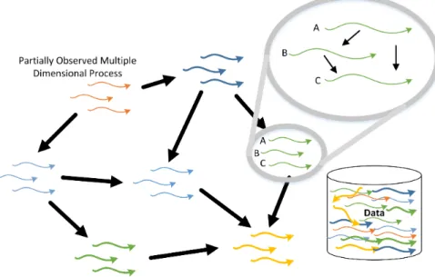
This leaves the task of being given a set of observable features (the data), that describe a set of latent processes, and recovering the underlying structure of the influence relations between these processes. More precisely, considerFigure2which
shows an example of a set of partially observed processes each given by3features (A, B, and C). Our task is to deduce the probability distribution that most likely resembles the model which generated the data. That is, we need to learn some structure between processes and parameter setting (which describe the probability of data values) that is capable to describe this temporal distribution. The structure of influence in this case is given by the black bold solid arrows.
Figure2: An influence structure between multi-dimensional processes. The colored solid ar-rows indicate features which describe processes and the black bold solid arar-rows indicate the influence between these processes.
A closer inspection of this problem reveals another learning task to identify the probability distribution for each individual multi-dimensional process with respect to the given set of observations. However, often we need to aggregate observable temporal features to tell us about high-level features which we can use to better describe each multi-dimensional process.
In this task we are only given the temporal features as data and are asked to deduce the dynamic probability distribution which explains the interaction between these
processes as illustrated by Figure 2. In scenarios where we have complete data we
often resort to maximum likelihood estimation (MLE), which optimises the likelihood function for a set of parameters that describes the processes with respect to the data. Unfortunately, in this case we are not given complete data and instead are given a set of partially observable processes, each with a set of temporal observations, that we want to discover the probabilistic structure of influence between. In this case the likelihood function has multiple optima which we can not optimise by just using the derivative of the likelihood function [Koller and Friedman2009].
Recovering the influence structure from temporal incomplete data, that is induced by a set of temporal observations, appears in most practical applications where we wish to perform density estimation to given observations; or learn the latent charac-teristics of an environment, which changes over time, for knowledge discovery (e.g. learning how traffic on roads in an area influence each other over time, or how the protein composition of a cell changes as its conditions change). In the next section we provide a brief overview of current practices in structure learning to address this problem.
1.3 ov e r v i e w o f l i t e r at u r e
As far as we know this particular problem has not been solved in current literature, however, several foundational learning practices can make our task simpler. In score-based structure learning we want to optimise a scoring function over different net-work configurations [Friedmanet al.1999]. That is, we use a structure score to search for the most suitable structure relative to the data. Most popular structure scores are variations on the likelihood score which calculates the probability of the data given a potential structure [Liuet al. 1996].
In observable data, the decomposability of the likelihood score [Carvalho et al.
2011], which is the ability to represent the score as a sum of variable family scores, allows for efficient learning procedures and significant computational saving [Koller and Friedman2009].Figure3 shows an example of how score-based structure
learn-ing can be used to select a network which makes the data ofX1, X2, X3, and X4 as likely as possible. The likelihood to the data is given by the score beneath each struc-ture. The structure with the highest score is selected since it has the highest likelihood relative to the training data.
In incomplete data, the likelihood score is not decomposable and we have to per-form inference to evaluate it [Tanner and Wong1987]. This forces us to use non-linear optimisation techniques, such as expectation maximization or gradient ascent [Binder
et al.1997], which are methods used to optimise the likelihood function with multiple optima [Dempster et al.1977]. Furthermore, local changes to the network can affect other parts of the network, which makes learning with incomplete data all the more difficult [Jordan1998]. Score-based structure learning provides a way to select an op-timal network for observable data but still leaves learning the latent aspects of the network open.
In this thesis we propose a score-based structure learning approach as being suited to the task of learning influence between partially observable processes since it can (a)
• • • X1 X2 X3 X4 30 X1 X2 X3 X4 20 • • • X1 X2 X3 X4 8
Figure3: An example of how score-based structure learning selects the best network struc-ture with respect to the data. The figure shows three strucstruc-tures each with a strucstruc-ture score below it. The shaded nodes represent observable variables. The highest struc-ture score is selected (circled in red) and the corresponding strucstruc-ture is used.
consider the complete influence structure between processes as a state in the search space; (b) preserve basic score properties allowing for feasible computations; and (c) provide a clear indication of the independence assertions between temporal models relative to the data. A complete literature review is provided inChapter3. In the next
section we discuss on overview of the proposed method to recover influence between processes.
1.4 ov e r v i e w o f m e t h o d
We note the major difficulty of this problem lies in the representation of the la-tent components of the influence network. In this thesis we develop an algorithm which learns the probability distribution that describes interactions between pro-cesses which manifest in the temporal observations that describe each process.
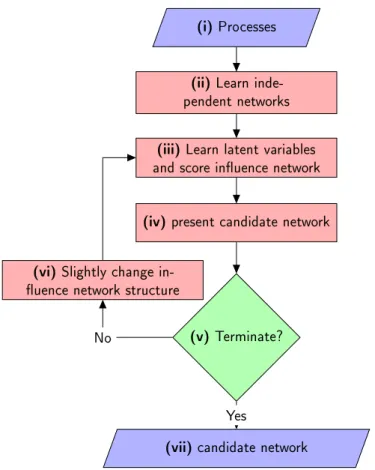
The high-level architecture of the proposed algorithm is given by Figure 4. The
general algorithm is as follows. We (i) input the processes; (ii) learn each stochastic process independently as a temporal model; (iii) relearn the parameters for an influ-ence network (with the new independinflu-ence assertions) by maximising the likelihood function for the hidden variables between the temporal models which represent each stochastic process; (iv) compute the structure score of the dynamic influence network; (v) check whether the condition to terminate the algorithm is met, either by conver-gence, some threshold, or if there is no way to improve the dynamic influence net-work relative to the data; (vi) slightly change the influence structure which encodes the distribution with the best possible change and continue with steps (iii), (iv), and (v). In (vii) we select the best candidate dynamic influence network.
Our method extends concepts in score-based structure learning for the domain of tracking influence between stochastic processes. We first factorise the distributions presented as stochastic processes into a set of temporal models. We then define an assembleand ascoring functionto evaluate the quality of candidate influence networks (Chapter 5). At this point we have a combinatorial optimisation problem which
re-quires us to traverse the search space for the optimal influence network, which we return as the goal structure that best fits the training data (Chapter 6). In the next
(i) Processes (ii) Learn inde-pendent networks (iii) Learn latent variables and score inuence network (iv) present candidate network
(v) Terminate? (vi) Slightly change
in-uence network structure
(vii) candidate network Yes
No
Figure4: An overview of the proposed algorithm to recover influence between stochastic processes represented as temporal networks.
1.5 n ov e lt y a n d c o n t r i b u t i o n
The novelty and intuition of our approach is to learn the influence structure in layers. We firstly learn a set of independent temporal models, and thereafter, optimise a structure score over possible structural influence configurations. Since the search for the optimal structure is done using complete data we can take advantage of efficient learning procedures and significant computational saving from the structure learning literature [Koller and Friedman2009].
We provide the following high-level contributions:
1. The notion of influence between processes. This includes the formulations of direct and delayed influence (Chapter4).
2. Several scoring function for dynamic influence networks by extending and adapting traditional scores for random variables along with their key properties (Chapter5).
3. The notion of a structural assemble to relate temporal models for dynamic in-fluence tasks (Chapter5).
4. A learning procedure to recover the influence structure between temporal mod-els with latent variables. We further extend the local search procedures to use assembles that link temporal models meaningfully while preserving decompos-ability and score-equivalence required for a manageable search (Chapter6).
5. We provide empirical evidence for the effectiveness of our method with respect to a generative ground-truth distribution (Chapter7).
1.6 t h e s i s s t r u c t u r e
This thesis is structured as follows. Chapter 2 provides the background work on
Bayesian networks and parameter estimation necessary to understand this thesis; Chapter3 provides relevant related work which served as the foundation for most
of the algorithms presented in this thesis.Chapter 4 defines influence between
pro-cesses and how to represent it using dynamic influence networks.Chapter5provides
the structure scores necessary to evaluate the worth of dynamic influence networks and introduces the notion of a structural assemble to relate temporal models. Chap-ter6provides learning and evaluation procedures that traverse the search space and
evaluate the learned model with respect to the ground truth generative model. Chap-ter7provides the results and discussion of this research. Finally,Chapter8presents
2
B A C K G R O U N D
2.1 i n t r o d u c t i o n
O
ur primary objective, in this thesis, is to track influence between stochastic processes. Stochastic processes are trajectories of complex statistical depen-dence that evolve over time and space [Doob 1953; Karlin 2014]. Common examples of stochastic processes include the exchange rate fluctuations [Bates1996], the stock market [Gardiner 1985], temperature [Van Kampen 1992], speech signals [Rabiner and Juang 1986], audio signals [Kim 2000], video signals [Moore and Essa 2002], etc.Figure5shows an example of the monthly price of brent spot crude oil asa stochastic process [Conget al.2008].
Figure5: Monthly price of brent spot crude oil, January 1995 to February 2016. Adapted from Independent Statistics & Analysis, U.S. Energy Information Administration (EIA) (Petroleum & Other Liquids) [Conget al.2008].
Stochastic processes can be modelled by relating random variables to each other over adjacent time-steps in dynamic Bayesian networks [Press1989]. Dynamic Bayesian networks can expressively represent probabilistic dependencies between random vari-ables over time, however, they present their own learning and representation prob-lems [Schweppe1973]. We explore the learning and representation of dynamic Bayesian networks in this chapter.
This chapter reviews the ground-work required to understand the content pre-sented in this thesis. All of the concepts outlined here are traditional probabilistic
graphical frameworks that have been developed and refined over many years [ Mur-phy and Russell 2002; Bishop2006; Koller and Friedman2009]. The intention of this chapter is to simply provide the reader with some context necessary to understand the developments of procedures presented in this thesis and are not intended to pro-vide a tour of the practices of probabilistic graphical models.
Additional readings for understanding the representation, inference, and reason-ing of probabilistic graphical models can be found in Koller and Friedman [2009]; Murphy and Russell [2002]; Pearl [1988]. In Section 2.2, we explore the
representa-tion of several Bayesian networks; and in Section 2.3, we present the fundamental
practices to learning Bayesian networks.
2.2 b ay e s i a n n e t w o r k s: r e p r e s e n tat i o n
Suppose that we are given astochastic processthat is parameterised by a set of random variables:X={X1,. . .,Xn}. Our goal is to represent a joint distributionPoverX. Rep-resenting this joint distribution is both technically and computationally demanding [Bailey1990;Sakamoto and Ghanem2002]. This is because controlling a distribution parameterised over such an extensive space would take a large amount of computer memory and would require a super-exponential amount of prior information elicited by an expert.
The exploration of independence properties and alternative parameterisation has allowed us to express sparse compact representations that we use to explore complex joint distributions. We begin with a useful tool, called Bayesian networks, that uses independence assertions to compactly express a joint distribution [Pearl2011].
Section2.2.1 establishes the representation of a Bayesian network along with
suit-able applications and groupings; and Section 2.2.2 expands the Bayesian network
representation into a template class of models that can describe complex statistical relationships over time.
2.2.1 Bayesian Networks
Representing probability distributions by graphical models has been explored before [Wright 1921 1934]. During these early innovations the joint probability distribution was described as influence between random variables encoded as a directed acyclic graphical structure which represented independence assertions [Smith1989;Howard and Matheson1984].
These developments gave raise to the notion of a Bayesian network which embeds independence assertions into a graphical structure together with a probability distri-bution. Pearl (and his colleagues) proposed the Bayesian network [Verma and Pearl 2013;Geiger and Pearl2013;Geigeret al.2013 1990]. We ascribe this preliminary work on Bayesian networks to the work laid out byPearl[1988].
Section2.2.1.1begins by defining the Bayesian network and discuses some
of I-maps and I-equivalence; and finally,Section2.2.1.3presents the simplest version
of a Bayesian network called a naïve Bayes model, showcases various applications of Bayesian networks, and presents the problem of eliciting the structure of a Bayesian network manually by an expert.
2.2.1.1 What is a Bayesian Network?
A Bayesian network is a directed acyclic graph (DAG) whose nodes represent random variables and whose edges represent the influence of one variable over another [Pearl 2011]. A Bayesian network structure is often established as a set of conditional inde-pendence assertions between these random variables that encode a joint distribution in a compact way [Pearl 1988; Koller and Friedman 2009]. Two random variablesX andYare said to be conditionally independent given a setZ, denoted(X ⊥⊥ Y |Z), if once we knowZ, then knowingXdoes not give us any information aboutY. We will use this notion of conditional independence to define the Bayesian network structure. Definition 2.1. A Bayesian network structure, GB, is a DAG whose nodes repre-sent random variables X1,. . .,Xn. Let PaGXB
i denote the parents of Xi in G
B, and NonDescendantsXi denote the variables in the graph that are not descendants ofXi
inGB. ThenGB encodes the following set of conditional independence assumptions, called local independencies, denoted byIl(GB):
∀Xi: (Xi⊥⊥NonDescendantsXi|Pa
GB Xi),
where⊥⊥denotes independence.
Figure 6 provides an example of a Bayesian network structure. The graph in
Fig-ure 6 is a DAG with six random variables represented as nodes. Four of these are
directly observed (observable, shaded) and two of these are not directly observed (la-tent, non-shaded). The influence between variables are represented as edges between them and are encoded as conditional independence assumptions.
X1
X2
X3
X4 X5
X6
Figure6: A Bayesian network with six random variables. VariablesX
1 andX2 are latent (not directly observed) and variablesX3,X4,X5, andX6are observed. The shaded nodes are called observable variables and non-shaded nodes are called latent variables. Entries in the joint distribution in Bayesian networks can be expressed as a product of factors [Jensen 1996]. A factor encodes the conditional probability distribution (CPD) of a random variable and is constructed with respect to its parent variable(s)
[Pepe and Mori1993].Figure7provides an example of a Bayesian network which is
used to predict the probability of the grass being wet given a set of variables [Pearl 2014]. Figure 7 explicitly presents each factor associated to each random variable.
We note that each factor presented has an associated dependency with respect to the network structure [Pearl 2014]. The variable for wet grass is dependent on the variables Rain and Sprinkler. Each factor is represented by a Bernoulli distribution [Hilbe2011] with values true (T) or false (F). We can condition on certain columns of the factor for Wet grass to give us more information about the distribution described.
Figure7: A Bayesian network showing the relationship between four random variables adapted fromPearl[2014]. Each node in the graph is a variable which is expressed
by a table called a factor. The factor for a variable contains all the possible values for that variable assigned to a probability, this is called a parameter. The product of all factors must be a legal probability distribution.
The ability to represent the joint distribution in terms of a factorisation in Bayesian networks, as shown in Figure 7, is a important contribution [Charniak 1991]. We present the following factorisation known as the chain rule for Bayesian networks [Pearl1988].
Definition2.2. LetGB be a Bayesian network structure over the variablesX1,. . .,Xn. We say that a probability distributionPBover the same space factorises according to
GB ifP
B can be expressed as a product PB(X1,. . .,Xn) = n Y i=1 P(Xi|PaG B Xi).
A Bayesian network is then just the conditional independences described by the Bayesian network structure and the distribution which is described by each variable’s factor [Pearl1988].
Definition2.3. A Bayesian network is a pairB= (GB,PB)where the distributionPB
factorises over the independence assumptions inGB.
Having defined a Bayesian network, we might consider performing reasoning or inference [Jensen1996;Zou and Feng2009;Cooper1990].Wellman[1990] crystallised
the three fundamental types of reasoning patterns in Bayesian networks: causal rea-soning, evidential rearea-soning, and inter-causal reasoning. These patterns can be used to promote knowledge elicitation and learning [Renooij and van der Gaag 2002; Hartemink et al. 2002] as well as the development of intuition to inference tasks [Druzdzel 1993]. The importance of reasoning patterns are emphasised by Pearl [1988]. In the next section we will see how two Bayesian network structures can decompose as the same set of independence assumptions.
2.2.1.2 I-maps and I-equivalence
Recall that our Bayesian network structure,GB, encodes a set of independence asser-tions,I(GB). Let us define these assertions more carefully:
Definition 2.4. Let P be a distribution over a set of random variables X. The set of independence assertions, denotedI(P), is a set of statements of the form(X⊥⊥Y |Z). These statements all hold inP.
GB is said to be an I-map of P since P satisfies the local independence assertions associated with the Bayesian network structureGB. We denote this as I(GB) ⊂I(P). More generally,
Definition2.5. LetGbe a graph structure and I(G) be its set of independence asser-tions.Gis said to be an I-map for a set of independencesIifI(G)⊆I.
Intuitively we view an I-map,G, as an incomplete indication about the set of inde-pendence assumptions that must hold inP [Koski and Noble2011]. However,P may contain additional independence statements that do not hold inG.
An important observation is that I(GB) provides an abstraction from the specific graphical structure to a set of independence assertions. This set stands to represent
GB as a specification of independence statements, which suggests that although two graphical structures, GB1 and GB2, may be semantically different, they could encode exactly the same set of conditionally independence assumptions, that is I(GB1) = I(GB2)[Koller and Friedman2009]. More formally,
Definition 2.6. Two Bayesian network structures, GB1 and GB2, over the same set of random variablesXare said to be I-equivalent ifI(GB1) =I(GB2).
It can be further stated that every possible configuration over the random variables
Xcan be partitioned into sets of mutually exclusive I-equivalence classes as defined in Definition 2.6. Figure8 shows an example of three graphical models that encode
exactly the same independence assumption: (A ⊥⊥ C | B). Notice that although the independence assumption is the same in all three networks, the edges can be oriented in different ways.
I-equivalence was defined byVerma and Pearl[1992];Judea Pearl[1991]. The con-tribution by Chickering [1995]; Verma and Pearl [1992]; Judea Pearl [1991] provide powerful tools to prove properties of I-equivalent graphical structures.
(a) B A C (b) B A C (c) B A C
Figure8: An illustration of three graphical models that encode the independence assumption:
(A⊥⊥C|B).
I-equivalence is undoubtedly an important concept when recovering influence re-lations since the true structure of a Bayesian network is seen as not identifiable from members of the I-equivalence class given observable data alone [Murphy2012;Koller and Friedman2009;Pearl 2011]. However, there are algorithms that can reconstruct the I-equivalence class given the observable distribution, such as those byPearl and Verma[1995];Verma and Pearl[1992];Spirteset al.[2000];Meek[1995].
In the next section we explore the simplest kind of Bayesian network structure and probability distribution, called the naïve Bayes model.
2.2.1.3 Naïve Bayes Model
Perhaps the simplest example of a Bayesian network is the naïve Bayes model [
Mc-Callum and Nigam1998] which has been used successfully by many expert systems
[De Dombalet al.1972;Gorry and Barnett1968;Warneret al.1961].
The naïve Bayes model predefines a finite set of mutually exclusive classes [Rish 2001]. Each instance (set of observations) can fall into one and only one of these classes, which is represented as a latent class variable. The model also poses some observed set of features X1,. . .,Xn. The assumption is that all of the features are conditionally independent given the class label of each instance [Murphy2012]. That is,
∀i(Xi ⊥⊥Xi0 |C), whereXi0 ={X1,. . .,Xn}−{Xi}.
Figure9presents the Bayesian network representation of the naïve Bayes model. The
joint distribution of the naïve Bayes model factorises compactly as a prior probability of an instance belonging to a class,P(C), and a set of CPDs which indicate the proba-bility of a feature given the class [Koller and Friedman2009],P(Xi |C). We can state this distribution more formally as
P(C,X1,. . .,Xn) =P(C)
n
Y
i=1
P(Xi|C).
The naïve Bayes model remains a simple, yet highly effective, compact, and high-dimensional probability distribution that is often used for classification problems [Shinde and Prasad2017; Lewis 1998; Duda and Hart 1973]. The main limitation of the naïve Bayes model is the assumption that all features are conditionally indepen-dent given the class variable.
Class X1 . . . Xn
Figure9: A graphical illustration of the naïve Bayes model.
The use of Bayesian networks span a range of applications including general diag-nostic systems [Andreassenet al.1987;Heckermanet al.2016;Breeseet al.1992]; event forecasting [Abramson1994;Guet al. 1994;West1996;Sunet al.2006]; assessment of short free-text responses [Kleinet al.2011]; machine vision [Levittet al.2013;Binford
et al.2013;Buxton1997]; manufacturing [Nadiet al.1991;Wolbrechtet al.2000;Weber and Jouffe2003], and emergency evacuation [Wanget al.2008] to name a few.
We have seen that the Bayesian network is an important tool for describing high-dimensional complex probability distributions and have outlined several successful applications. However, manually eliciting the conditional probability distribution (CPD) and network structure is a complex task that has plagued decision analysis for many years [Chesley 1978; Spetzler and Stael von Holstein 1975]. This difficult process is subject to many biases [Tversky and Kahneman1975; Daneshkhah 2004] and although some contributing methods can be used to obtain the network structure and parametrisation from an expert [Schachter and Heckerman1987], this remains a difficult processes.
In this subsection we explored the Bayesian network representation as a powerful tool to describe environments for numerous applications. In the next section we will extend this descriptive language for the temporal setting.
2.2.2 Dynamic Bayesian Models
Bayesian networks can be used to model a joint distribution over a set of random variables [Koski and Noble 2011]. In temporal settings, however, we wish to model distributions over trajectories (systems that change over time) [Murphy and Russell 2002].
For example, suppose we are interested in capturing the traffic condition of a road over time [Jayakrishnanet al.1994]. Then we would be interested in building a distri-bution of features over different time-slices with respect to some time granularity to capture the distribution of traffic over time [Papageorgiou1990].
In such cases it is often useful to construct a template model which unrolls as the trajectory evolves over time [Conati et al. 2002]. In this section we explore the rich and expressive language of dynamic Bayesian networks which can be used to describe distributions over trajectories [Pavlovicet al.1999;Dojeret al.2006].
Section2.2.2.1andSection2.2.2.2explore two common assumptions that are made
when dealing with dynamic Bayesian networks; Section 2.2.2.3 introduces the
lan-guage of dynamic Bayesian networks and explores some notable applications and practices of dynamic Bayesian networks; and finally,Section2.2.2.4presents a
partic-ular class of dynamic Bayesian networks which organises its random variables as a hierarchy.
2.2.2.1 Markov Systems
In this section we will consider dynamic Bayesian networks to represent systems that evolve over time. The dynamic Bayesian network is a temporal model represented by a set of template variables, denotedX. We will denote the values of the template variablesXiat timetasX(it).
A stochastic process can be viewed as a trajectory over a set of discrete time steps specified by a time granularity. Over this time granularity, we can model the relation-ship between these time-slices using the chain rule for probabilities (Definition 2.2)
[Koller and Friedman2009] as,
P(X(0:T)) =P(X(0))
TY−1 t=0
P(X(t+1)| X(0:t)).
AsT increases,P(X(0:T)) exponentially increases the number of independence as-sumptions over the trajectory length. Thus, a simplifying assumption is to model the next state as conditionally independent of the past given the present. We present the notion of a Markov system.
Definition 2.7. A dynamic system is said to be Markov, over the set of template variablesX, if for allt>0,
(X(t+1)⊥⊥X(0:(t−1)) | X(t)).
We note that use of the Markov assumption is a reasonable approximation if we use a rich description of the system state [Koller and Friedman 2009; Murphy and Russell2002]. That is, increasing the number of variables which describe each time-slice might allow us to describe influences which persist through time.
2.2.2.2 Time Invariance
The Markov assumption simplifies the distribution over time, however, we need to make one more simplifying assumption about the general representation of the tem-poral model [Koller and Friedman2009;Murphy and Russell2002].
Definition2.8. A Markov system is said to betime invariantifP(X(t+1) | X(t)) is the same∀t. That is∀t>0, we describe the process as the transition modelP(X0|X)as
P(X(t+1)=ξ0| Xt =ξ) =P(X0=ξ0 | X=ξ),
whereξ0 is the next data instance andξis the current data instance.
With these assumptions in hand we can define a dynamic Bayesian network in the next section.
2.2.2.3 What is a Dynamic Bayesian Network?
The assumptions made in the previous section allow us to compactly represent a trajectory over time [Murphy and Russell2002]. It is compact since we need to only specify a 2-time-slice Bayesian network that consists of the initial distribution and a transition model, P(X0|X) [Koller and Friedman 2009]. The transition model can then be unrolled using the Markov and time invariance assumptions into a dynamic Bayesian network. We begin by defining the2-time-slice Bayesian network.
Definition2.9. A2-time-slice Bayesian network for a process over the set of template variablesXis a Bayesian network overX0givenXI, whereXI⊆Xis a set of interface variables.
The conditional Bayesian network described only has parents and hence CPDs for X0. Interface variables refer to those variable that persist through the temporal aspect of the model (e.g. high-level changes in the process). Using our simplifying assumptions, the distribution defined can be described as
P(X0|X) =P(X0|XI) = n Y i=1 P(Xi0|PaX0 i). ( 1)
Consequently for every template variable we will have a template factor (Sec-tion2.2.1.1) which will be initialised as the model unfolds. There are generally two
types of edges defined in these models [Koller and Friedman 2009; Murphy and Russell2002]:
• time-slice edges, which describe dependencies between time-slices. Inter-time-slice edges that are between copies of the same template variables are called persistent edges. We refer to variables with persistent edges as persistent variables.
• Intra-time-slice edges describe dependencies within each time-slice.
We now provide a definition of the unrolled dynamic Bayesian network which uses the notion of a2-time-slice model.
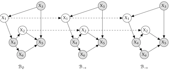
Definition2.10. A dynamic Bayesian network (DBN) is a pairhB0,B→i, whereB0 is a Bayesian network overX(0), representing the initial distribution over states andB→ is a 2-time-slice Bayesian network for the process. For any desired time span T >0, the distribution over X(0:T) is defined as an unrolled Bayesian network, where, for anyi=1,. . .,n:
• the structure and CPDs ofX(i0)are the same as those forXiinB0,
X1 X2 X3 X4 X5 X6 B0 X1 X2 X3 X4 X5 X6 B→ X1 X2 X3 X4 X5 X6 B→
Figure10: A dynamic Bayesian network with six template variables. BothX1andX2are per-sistent variables connected by dotted intra-time-slice perper-sistent edges. The shaded template variables are observable and not a part of the interface set. The network is unrolled over three time-slices. Below each time-slice there is an indication from which model in the2TBN it is derived from.
Figure10 shows an example of an unrolled dynamic Bayesian network. Temporal
models over trajectories have been discussed for many years, such models include hidden Markov models (HMMs) [Rabiner and Juang 1986; Rabiner 1989], Kalman filters [Kalman 1960], and possibly the first formal occurrence of dynamic Bayesian
networks (DBNs) in Dean and Kanazawa [1989]. The connections between HMMs
and DBNs have also been explored [Smyth et al. 1997].Murphy and Russell [2002]; Koller and Friedman[2009];Murphy[2012] provide an overview of temporal repre-sentations and DBNs.
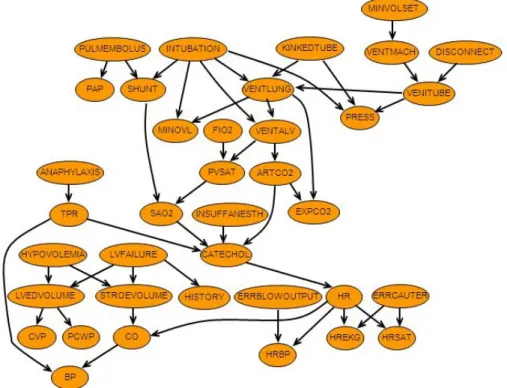
DBNs have been used for dependability, risk analysis, and maintenance [Weberet al. 2012]; speech recognition [Zweig and Russell 1998]; recognising office activities [Oliver and Horvitz2005]; vehicle classification in video [Kafai and Bhanu2012]; the analysis of football matches [Huang et al. 2006]; and even in genetics, where DBNs capture temporal expression data to uncover gene interaction in cellular systems1
[Friedmanet al.2000].
2.2.2.4 Hierarchical Bayesian Networks
DBNs are able to model trajectories of complex statistical dependences that evolve over time [Murphy and Russell 2002]. These are modelled by relating variables to each other over adjacent time-steps [Murphy and Russell 2002]. DBNs expressively represent probabilistic dependencies between variables but can be redefined to ex-press dependencies between composite variables, which are mixtures of other vari-ables [Peelenet al. 2010]. This is useful in situations when we wish to learn abstrac-tions of a subset of observaabstrac-tions for a process. We extend the definition of DBNs
1 This is done using DNA hybridization arrays which estimate the expression levels of thousands of
into hierarchical dynamic Bayesian networks (HDBNs) which expresses composite variables naturally in temporal models.
Hierarchical Bayesian networks (HBNs) are used extensively for reasoning under uncertainty with structured data [Gelman et al. 2014]. In this section we extend the HBN to one which expresses uncertainty over structured data over time. The major contribution of HBNs lies in their expressive power to aggregate random variables as composite structures of other variables [Gelmanet al.2014;Peelenet al.2010;Murphy and Russell2002]. We begin by defining a composite variable.
Definition2.11. A variable,X, is said to be a composite variable if it has a component set{X1,. . .,Xn}of variables.
These composite variables can be expressed recursively to construct complex hier-archical tree (h-tree) structures.
Definition 2.12. A hierarchical tree (h-tree) structure of a composite variable X, de-noted hX, is a directed tree structure rooted at X, with each of the elements in X’s component set being children of X expanding along with each of the component’s respective h-trees.
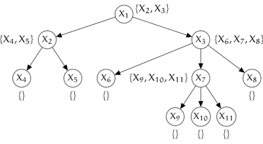
Gyftodimos and Flach [2002] provide an overview of hierarchical models using composite types. Figure 11 shows an example of a simple hierarchical structure for 11 composite variables. Each composite variable, alongside its factor that describes a distribution, also contains a set of composite variables which are dependent on it given the hierarchical structure. Leaf nodes have empty composite variable sets since they are at the lowest level of the hierarchy. These are usually observable. We now formally define a HBN structure using this notion of a h-tree.
Definition2.13. A hierarchical Bayesian network structure of a composite variableX
with corresponding h-tree structure is a set HX = {hX1,. . .,hXn}, where hXi is the
corresponding h-tree for theith component ofX.
A hierarchical Bayesian network is simply a distribution which factorises over this hierarchical structure. More formally,
Definition 2.14. A hierarchical Bayesian network is pair H = (HX,PHX) where PH
X1 { X2,X3} X2 {X4,X5} X3 {X6,X7,X8} X4 {} X5 {} X6 {} X7 {X9,X10,X11} X8 {} X9 {} X10 {} X11 {}
Figure11: A hierarchical Bayesian network structure for11random variables. Each variable is a data-structure made up of a factor and a set of composite variables. The factor describes the conditional probability distributions (CPDs) and the set of composite variables contain the child variables relative to the structure.
An inherited property of hierarchical Bayesian network structure from standard Bayesian network structures is outlined in Definition 2.1. We now naturally extend
this definition for hierarchical dynamic Bayesian networks (HDBNs) for structured time-series data.
Definition2.15. A2-time-slice hierarchical Bayesian network (2-THBN) for a process over a set of composite variablesX is a hierarchical Bayesian network over Xgiven
XI, whereXI⊆Xis a set of interface variables.
We can now adopt the Markov and time invariance simplifying assumptions to define the hierarchical dynamic Bayesian network (HDBN).
Definition2.16. A hierarchical dynamic Bayesian network (HDBN) is a pairHDB =
hH0,H→i, where H0 is a hierarchical Bayesian network over X(0), representing the initial distribution over states andH→ is a2-THBN for the process. For any desired time span T > 0, the distribution over X(0:T) is defined as a unrolled hierarchical Bayesian network, where, for anyi=1,. . .,n:
• the structure and CPDs ofX(i0) are the same as those forXiinH0,
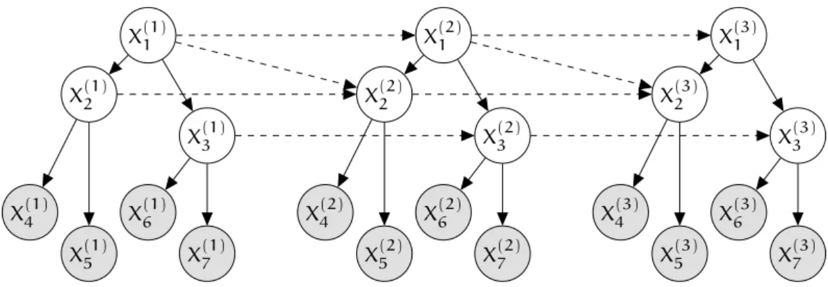
• the structure and CPDs ofX(it)fort > 0are the same as those forXi0 inH→. Figure12illustrates an example of a HDBN with3time-slices and7template
vari-ables. Some inter-time-slice edges are persistent and some persist to other varivari-ables. The main strength of HDBNs is its ability to represent uncertainty in structured data by aggregating variables in high-level features, this allows us to describe a rich prob-ability distribution through the abstraction of observations even in the presence of incomplete data.
X(11) X(21) X(31) X(41) X(51) X(61) X(71) X(12) X(22) X(32) X(42) X(52) X(62) X(72) X(13) X(23) X(33) X(43) X(53) X(63) X(73)
Figure12: A hierarchical dynamic Bayesian network with three time-slices and seven vari-ables per time-slice (3latent and4observable). The inter-time-slice edges (dashed lines) are sometimes non-persistent which can enrich the distribution. The intra-time-slice edges (solid lines) describe the hierarchical structure which is captured in these models.
2.3 b ay e s i a n n e t w o r k s: l e a r n i n g
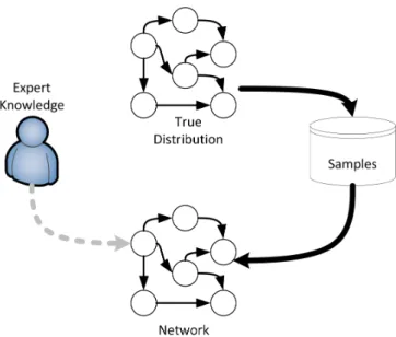
In this section we explore the task of learning Bayesian networks from data. Fig-ure 13 shows the context of the learning process. Suppose we observe (or partially
observe) atrue distribution(P∗) as shown in Figure13. We may also assume that the
true distribution,P∗, is generated from a true network structure (G∗). That is, a set of independence assumptions from which the true distribution is an I-map. From the true distribution we are able to obtain a set of samples. We might also have access to domain expertise which together with the samples generated will allow us to learn a network. Domain knowledge can come in the form of information about the structure between variables or possibly the general structure of a distribution of the involved variables. Hastie et al. [2001]; Bishop [2007] provide an overview of basic learning problems and algorithms in Bayesian networks.
The motivation behind learning Bayesian networks is primarily for density estima-tion [John and Langley1995;Fraley and Raftery2002], to make predictions over new instances, and as a framework for knowledge discovery [Fayyad et al.1996; Hecker-man1996], that is, learning how variables may interact.
There are four different contexts of learning in Bayesian networks [Koller and Fried-man 2009]: we may have (a) a known structure with complete data; (b) unknown structure with complete data; (c) known structure with incomplete data; or (d) un-known structure with incomplete data. We begin by discussing the learning problems (a) and (c) in Section2.3.1, and leave structure learning problems (b) and (d) to be
discussed with the related work in the next chapter.
2.3.1 Parameter Estimation
In this section we explore various parameter estimation learning algorithms. We be-gin be discussing maximum likelihood estimation (MLE) [Scholz1985;Johansen and
Figure13: An illustration of the process of learning a Bayesian network from domain exper-tise and samples that are generated from a true distribution. Adapted fromKoller and Friedman[2009].
Juselius1990] inSection2.3.1.1, which optimises the likelihood function for complete
data. MLE is perhaps the most commonly used parameter estimation tool available [Lehn 2017; Scholz 1985; Enders and Bandalos 2001]. We then explore Bayesian es-timation in Section 2.3.1.2, which is based on the Bayesian paradigm which states
that anything we have uncertainty over should be expressed as a distribution [Shafer 1976].
We also address the problem of learning the parameters of DBNs which are used to express a distribution over trajectories [Koller and Friedman2009;Murphy and Rus-sell2002]. We will see that temporal models are extensions of Bayesian learning due to the simplifying assumptions (Section2.2.2.1and2.2.2.2). Finally, inSection2.3.1.3,
we address learning with incomplete data, which is a much harder problem.
2.3.1.1 Maximum Likelihood Estimation
Perhaps the simplest parameter learning problem is maximum likelihood estimation (MLE) from a set of observations [Scholz1985]. MLE is foundational to many param-eter learning problems and much work has been dedicated to its development [ DeG-root and Schervish2012;Schervish2012;Hastieet al.2001;Bishop2007;Bernardo and Smith2001].Howard[1970] provides a tutorial on maximum likelihood estimation.
Suppose we are given a set of observations in the form of a datasetD={ξ1,. . .,ξM}
sampled independently and identically distributed (IID) from P∗. That is, the in-stances are independent of each other and sampled fromP∗ [Hoadley1971;Gänssler and Stute1979]. Our goal is to find the set of parameters,Θ, that predictsD. In order to address this we often look at the likelihood of the parameters with respect to the data [Scholz1985;Hastieet al.2001;Bernardo and Smith2001]. For example, suppose
that our data consists of a single observation,x, per instance,ξ, then the likelihood of the parameters relative to the data is given by
L(θ:D) =P(D|θ) =
M
Y
m=1
P(x[m]|θ). (2)
The likelihood which is assigned to a particular parameter can be calculated by using the notion of a sufficient statistic [Koller and Friedman2009].
Definition2.17. A functions(D) is a sufficient statistic from instances to a vector in
RK, whereK is the total number of values forX, if for any two datasets Dand D0 and anyθ∈Θwe have
X
x[i]∈D
s(x[i]) = X
x[i]∈D0
s(x[i]) =⇒ L(θ:D) =L(θ:D0).
In other words for any two datasetsDandD0, and any parameterθ, we have that if the sum of all of the sufficient statistics over all the instances in both datasets are the same, then their likelihood functions are the same [Koller and Friedman 2009]. We can express the likelihood of the parameters relative to the data as
L(θ:D) = k Y i=1 θMi i , (3)
whereθiis the parameter forx=x[i]andMiis the sufficient statistic of observation
x[i]. This distribution in the above equation is for a multinomial distribution. To choose the MLE for the parameter,θ, we simply find the optimum, ˆθ, which yields
ˆ
θi= PmMi
i=1Mi
. (4)
Note thatEquation4is just the fraction of the valuexiin the data represented by its
respective sufficient statistic.
MLE is considered a simple way to select a parameter that predicts D. The pa-rameter is constructed by using sufficient statistics which represent the key statistical properties of the datasetDwith computational efficiency and provides a closed form solution. Heckerman [1998]; Buntine [1996 1994] provide several tutorials on this foundational concept.
Although learning the parameters of independent events could be easily done us-ing MLE, Bayesian networks seem to present a significantly more difficult parameter learning problem. In Bayesian network parameter learning we are interested in mod-elling complex conditional distributions. As it turns out learning parameters for a Bayesian network is not significantly harder than learning the parameters for inde-pendent variables since the likelihood function is decomposable with respect to the network’s independence assumptions.
More specifically, Equation 2 presents the likelihood over a single variable.
Sup-pose we extend this formula for the likelihood of all variables in a network given its particular structure. We can express the likelihood of all of the variables, givenD using the chain rule for Bayesian networks as inDefinition2.2,
L(Θ:D) =Y
m
Y
i
P(xi[m]|Ui[m] :Θi),
where Ui is the set of parent values forxi with respect to the structure (iindicates the variable number and mindicates the instance number). We can now switch the order of the products from a product over variables to a product over data instances [Koller and Friedman2009],
L(Θ:D) =Y
i
Y
m
P(xi[m]|Ui[m] :Θi).
Therefore the likelihood of the parameters relative to the data is
L(Θ:D) =Y
i
Li(D:Θi),
which yields the likelihood of each family of variables individually. The decompos-ability of the likelihood function can be further exploited by using table CPDs (which is omitted here. For further reading on the decomposability of the likelihood term for Bayesian networks please consultMurphy and Russell [2002];Bishop [2006]; Koller and Friedman[2009]).
We can also use MLE when dealing with temporal models. Suppose we are given the following Markov chain [Kemeny and Snell 1960; Gilks et al. 1995] as shown in Figure14.
Figure14: A Markov chain over four time-slices. The parameter for each variable is explicitly shown by the blue node. Adapted fromConati[2002].
Given the time invariance assumption (Definition 2.8), we can describe the
tem-poral process as a transition model P(X0|X). Thus we can describe the likelihood function as L(θ:X0:T) = T Y t=1 P(X(t)|X(t−1):θ).
If we consider how the temporal model decomposes over pairs of states Xi andXj, then we can reformulate the product as
L(θ:X0:T) =Y
i,j
Y
t:X(t)=Xi,X(t+1)=Xj
In this case we are considering the probability over each transitionXitoXj. Given the time invariance assumption we note that the parameters for the model are the same regardless of which time point we consider. Therefore, can rewrite the likeli-hood function as a product over pairs of time-slices given the particular sufficient statistic. That is, forXa multinomial random variable andθ∈R,
L(Θ:X0:T) =Y i,j Y t:X(t)=Xi,X(t+1)=Xj θXi→Xj = Y i,j θM[Xi→Xj] Xi→Xj .
Similarly, we can extend this to the context of HMMs [Eddy1996], such as the one inFigure15. The likelihood function for the HMM decomposes as
L(Θ:X0:T,O0:T) =Y i,j θMXi[→XXi→jXj] Y i,k θMOk[|XXii,Ok], (5)
where X and O are multinomial random variables, θ ∈ R, with the additional pa-rameters which correspond to the observation k in the statei exponentiated by the number of times we observe bothXiandOk [Blunsom2004].
X(0) X(1) O(1) X(2) O(2) X(3) O(3)
Figure15: An illustration of a hidden Markov model with 4 time-slices. The dotted lines indicate the inter-time-slice edges for the persistent variable X(t). The solid line indicate the intra-time-slice edges for each respective time-slice.
To summarise, MLE provides a mechanism to select a parameter which makes the data as probable as possible. The convenience lies in its decomposability into local likelihood functions per observable family variable.
When optimising the likelihood function one must be careful of fragmentation, which states that as the number of parents increase, the number of possible assign-ments for each variable increases exponentially. This concept leads to poor parameter estimates in the severe cases. In such cases we might be able to perform better at den-sity estimation by considering simpler structures even if they may be incorrect [Koller and Friedman2009;Murphy and Russell 2002; Bishop2006]. In the next section we explore an extension to MLE which provides a Bayesian alternative.
2.3.1.2 Bayesian Learning
An alternative to MLE for learning the parameters of variables in a Bayesian network isBayesian estimation[John and Langley1995;Heckerman1998]. Bayesian estimation follows the Bayesian paradigm which views any event which has uncertainty as a random variable with a distribution over it [Shafer1976].
The naïve Bayes model, illustrated inFigure9, for classification is an early
to estimate the most likely parameterθrelative to the data, in Bayesian estimation we view the parameterθas a continuous random variable (θ∈[0,1]). Each instance,ξ, is viewed as conditionally independent given θ. However, since θis not known (what we are trying to learn), the instances are not marginally independent and information about every instance should tell us something aboutθ. Figure16illustrates how the
dataset is dependent on the parameterθ which updates its values as more data is acquired over time.
θ
ξ[1] . . . ξ[M]
Figure16: A graphical depiction of Bayesian estimation which views the parameterθ as a random variable. All the data instances are dependent onθ.
As an example considerFigure 17 which shows a simple Bayesian network with
two random variables G and R. Here we see that the parameter valuesθG andθC|G
are expressed explicitly as random variables in the model.Buntine[1994];Gilkset al. [1994] were the first to introduce Bayesian estimation for temporal models in terms of the template model representations.
Figure17: An example of a Bayesian network with variable parameters explicitly indicated as continuous random variables (blue nodes). The observable variables are indicated by the white nodes and the blue nodes explicitly indicate the parameters. Adapted fromWanget al.[2008].
Suppose each instanceξcontains only one observationx, then we can express the joint distribution of each observation by using the chain rule for Bayesian networks (Definition2.2) and the dependencies specified inFigure16as
P(x[1],. . .,x[M],θ) =P(x[1],. . .,x[M]|θ)P(θ).
Which gives us the prior overθand the probability of each instance givenθ,
P(x[1],. . .,x[M],θ) =P(θ)
M
Y
i=1
We note some similarities to MLE inEquation2 with the addition of the prior
prob-ability overθ. The prior distribution allows us to express the posterior of this prior given the data using Bayes rule:
P(θ|x[1],. . .,x[M]) = P(x[1],. . .,x[M]|θ)P(θ) P(x[1],. . .,x[M]) .
There are many choices for a prior distribution. One common choice is the Dirichlet prior which is characterised by a set of hyper-parameters(α1,. . .,αk). The Dirichlet prior for Bayesian networks was defined by Heckermanet al. [1995a]. The Dirichlet probability distribution is described as a density function overθwhich has the form
P(θ) = 1 Z k Y i=1 θαi−1 i , where Z= Qk i=1Γ(αi) Γ(Pki=1αi), Γ(x) = Z∞ 0 tx−1etdt. (6)
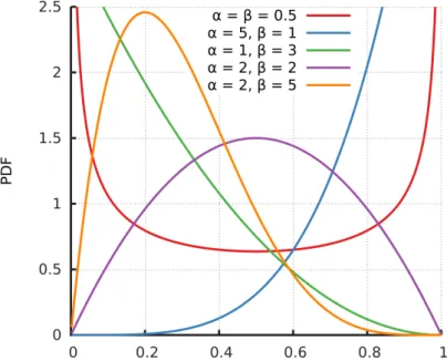
Figure 18 shows several examples of a special case of the Dirichlet distribution
with two hyper-parametersαandβ(also called a beta distribution). We note that as we increase the hyper-parameter values while α= β, we get a peak at the center of the x-axis. This corresponds to a stronger belief that the parameters are positioned around the center (e.g. whenαandβare both2).
Figure18: Examples of various Dirichlet Priors. Adapted fromHoras[2014].
Let us now consider how the Dirichlet prior updates as we receive more evidence for a particular event. The Dirichlet prior, inEquation6, and the likelihood function,
inEquation3, have the same form and so multiplying them gives us
k
Y
i=1
θMi+αi−1
i .
Therefore the posterior distribution is simply Dir(α1+M1,. . .,αk+Mk), whereMi

![Figure 7: A Bayesian network showing the relationship between four random variables adapted from Pearl [ 2014 ]](https://thumb-us.123doks.com/thumbv2/123dok_us/1437444.2692535/26.892.253.623.296.575/figure-bayesian-network-showing-relationship-random-variables-adapted.webp)