Simple Semi-Supervised Learning for Prepositional Phrase Attachment
Gregory F. Coppola, Alexandra Birch, Tejaswini Deoskar and Mark Steedman School of Informatics
University of Edinburgh Edinburgh, EH8 9AB, UK [email protected]
{abmayne, tdeoskar, steedman}@inf.ed.ac.uk
Abstract
Prepositional phrase attachment is an im-portant subproblem of parsing, performance on which suffers from limited availability of labelled data. We present a semi-supervised approach. We show that a discriminative lexical model trained from labelled data, and a generative lexical model learned via Expectation Maximization from unlabelled data can be combined in a product model to yield a PP-attachment model which is bet-ter than either is alone, and which outper-forms the modern parser of Petrov and Klein (2007) by a significant margin. We show that, when learning from unlabelled data, it can be beneficial to model the generation of modifiers of a head collectively, rather than individually. Finally, we suggest that our pair of models will be interesting to com-bine using new techniques for discrimina-tively constraining EM.
1 Introduction
Labelled data for NLP tasks will always be in short supply. Thus, a statistical parser trained with labelled data alone will always be troubled by unseen events—primarily when parsing out-of-domain data, or when faced with rare events from in-domain data. Thus, a major focus of current work is the use of cheap, abundantunlabelled data to improve state-of-the-art parser performance.
We focus on an important sub-problem of parsing—prepositional phrase attachment—and demonstrate a successful semi-supervised learn-ing strategy. We show that, uslearn-ing a mix of la-belled and unlala-belled data we can improve both the in-domain and out-of-domain performance of a prepositional phrase attachment classifier.
Prepositional phrase attachment, for us, is the decision as to which heads a series of prepositional phrases of the form [PP prep NP]modify, as in,
e.g.,
He ate a salad [PPwith a fork] [PP of plastic]
Prepositional phrase attachment is an important sub-problem of parsing in and of itself. Structural heuristics perform poorly (cf., Collins and Brooks, 1995), and so lexical knowledge is crucial.
Moreover, the highly lexicalized nature of prepositional phrase attachment makes it a kind of microcosm of the general problem of learning de-pendency structure, and so acts as a computation-ally less-demanding testing ground on which to try out learning techniques. We have endeavoured to approach the problem with a strategy that might be likely to generalize: a mix of generative and discriminative lexical models, trained using tech-niques that have worked for parsers.
The main contributions of this paper are:
• We compare the performance on the preposi-tional phrase attachment task of natural lexi-calized dependency parsing strategies, to the popular semi-lexicalized model of Petrov and Klein (2007), and show that a lexical is more effective for this problem.
• We show that a discriminative lexical model trained from labelled data and a generative lexical model learned through Expectation Maximization on unlabelled data can per-form better in a product model than either does alone, yielding a significant improve-ment over our baseline reference, the parser of Petrov and Klein (2007).
• We show that, in this case, when learning from unlabelled data, a strategy of generat-ing all modifiers of a headcollectivelyworks better than generating them individually.
2 Prior Work
Work on the topic of prepositional phrase attach-ment typically views the problem as a binary clas-sification task. Given a4-tuple,
hverb,noun1,prep,noun2i
the task is to decide whether the attachment of the [PPprep NP] prepositional phrase
character-ized byhprep,noun2iis toverbor tonoun1.
Human performance on this prepositional phrase attachment task has been estimated by Rat-naparkhi et al. (1994). They found that treebank-ing experts given the4-tuple binary decision task choose the correct attachment88.2%of the time. And, when then given the full context for the same examples, they choose the “correct” attachment (i.e. the same attachment that is given by the Penn Treebank)93.2%of the time.
Approaches to training from labelled data include rule-based (Brill and Resnik, 1994), maximum-entropy (Ratnaparkhi et al., 1994), and a generative “backed-off” model (Collins and Brooks, 1995).
The state-of-the-art is an approach by Stetina and Nagao (1997). They replace each noun and verb by a WordNet sense using a custom word sense disambiguation algorithm. Then, they train a decision tree on labelled WSJ data. Their method achieves essentially a human level of ac-curacy on this task: 88.1%. Toutanova et al. (2004) achieve a comparable result with a method that integrates word-sense disambiguation into the generative attachment model.
There is also a variety of work that makes use of unlabelled data to learn prepositional phrase attachment. An early example in this category is Hindle and Rooth (1991). They estimate the probability that a given preposition modifies a given head using an iterative process with hetero-geneous steps. Ratnaparkhi (1998) uses determin-istic heurdetermin-istics.
The state-of-the-art in this area is due to Pan-tel and Lin (2000). They, use a homespun iterative algorithm learning algorithm which bears a resem-blance to EM, but it does not seem to learn a gen-erative model. One interesting feature of this ap-proach is that the attachment decision for a given word is allowed to make use of the statistics col-lected forsimilar words, which helps to the spar-sity that occurs even in a large, unlabelled corpus.
Their performance on the binary classification task is84.5%.
We are aware of one case that has used a mix of labelled and unlabelled data: Volk (2002) uses a back-off strategy in which information from la-belled data is used when conclusive, and informa-tion from unlabelled data otherwise. Performance on the same task on a NEGRA-based data set lags behind the others, at81.0%.
Finally, Atterer and Sch¨utze (2007) argue that an experimental setup that evaluates a prepo-sitional phrase attachment with possible attach-ments given by an “oracle,” rather than an actual parser, may make the problem appear easier than it really is. This is a good point. But, for the pur-poses of comparing learning techniques, we feel that the typical oracle task is better suited, as it avoids introducing the noise of parser mistakes.
3 Background
3.1 The Prediction Task
We treat prepositional phrase attachment as a structured prediction task, rather than as a binary decision. The input to the prediction procedure will be a (prepositional phrase)attachment prob-lem, a string matching either the regular expres-sion (1) or (2).
(1) verb baseNP (prep baseNP)∗
(2) baseNP (prep baseNP)∗
For example, some attachment problems are:
(3) sought man from Germany with expertise
(4) man from Germany with expertise
Though not indicated above, we assume that POS tags are given as part of the problem, and need not be predicted.
Our goal is to create a prediction procedure which, given an attachment problem,x, will return a derivation, d, which is a parse for xusing the following mini CFG grammar whose initial sym-bol is ROOT:
(5) a. ROOT→VP
b. ROOT→NP
c. VP→verbHNP PP∗
d. NP→baseNPHPP∗
The head of each XP is indicated with a sub-scripted H. All siblings to a head are called its modifiers.
Given a full parse tree in the style of Marcus et al. (1993),attachment problem-derivationpairs were extracted using a TGrep-like functional pro-gram, which is described in Appendix A.1
3.2 Scoring Performance
When evaluating a prediction procedure, we will give it a series of attachment problems and ask for the derivations. In most cases, the score we will focus on is what we can call the binary decision score, i.e., the percentage of the time in which the first prepositional phrase following a verb–direct-object pair is attached correctly. In this case, we are reporting the same score as is typically re-ported on this task, so as to avoid introducing a new metric.
To be clear, then, when scoring, in this way,
[VPset[NPrate [PPon [NPrefund]]][PPat [NP5 percent]]]]
we only ask where [PP on [NP refund]] attaches,
and ignore the attachment decision of [PP at [NP5
percent]].
One might thus ask what the point of bother-ing with the whole derivation is if we are typically only intending to score a binary decision. Well, our model in§5.2 makes each attachment decision independently, and in this example from the WSJ development test set, incorrectly attaches bothon refund and at 5 percent to the verb. In contrast, our model of §5.3 attaches prepositional phrases collectively, and rejects the derivation where on refund and at 5 percent both modify set. Thus, though we only score one decision in a derivation, that decision can be influenced by others, and so it does make a difference to work at the level of derivations.
3.3 Data Sets
The traditional semi-supervised learning task in-volves learning from two sets. The first is a set of pairs,{(xi,di)}, of data points along with their
la-bels. The second is a (typically much larger) set of data points alone,{xj}(i.e. without labels). In our
case, the data points are attachment problems and the labels, which are structured, are derivations.
1Our data sets extracted from the Penn Treebank will be
available on request to those with the relevant license(s) to use Penn Treebank data.
Our experiment is interested in performance across domains. Thus, we also distinguish be-tween in-domain labelled data, some of which we will allow ourselves to use to train model param-eters, and out-of-domain labelled data, which we will not use to train model parameters.2
Our source of labelled data is the Penn Treebank (Marcus et al., 1993). We use sections0-22of the WSJ portion of the Penn Treebank for training and development and sections23,24are left for final evaluation. We variously use i) sections 2-21 as labelled training data, with sections 0,1,22 as a development test set, or ii) sections 0,1,5-22 as labelled data with sections2-4as held-out set for parameter tuning.
We split up the Brown portion of the treebank similarly to Gildea (2001)—i.e. we split it into10
sections such that thes’th sentence is assigned to sections mod 10. We then use sections 0-2 de-velopment test set,4-6for tuning, and sections7-9
are left for final evaluation. Our divisions of the Penn Treebank are chosen to resemble the canoni-cal training-test split for parsing, but we use more sections for testing, to obtain more reliable test scores, as there are far fewer decisions to test on in each section in our task, when compared to pars-ing.
Our source of unlabelled data is the New York Times portion of the GigaWord corpus (Graff et al., 2005). These sentences are parsed automati-cally using the generative semi-lexicalized parser of Petrov and Klein (2007). We did some filter-ing of these unlabelled sentences, removfilter-ing sen-tences with quotations (as quoted material can be ungrammatical) and sentences over 40 words in length (to increase the chance that each automatic parse used was reasonable).
We use these automatically extracted parses only to identify attachment problems (x), which we will then treat as unlabelled. That is, while there is possibly information in the derivations (the d) that the parser is coming up with, we did not use this.
In terms of size, our WSJ2-21 set has29,750
examples. The GigaWord set has8,038,001 ex-amples.
2
3.4 Baseline
Much past work has tested on the 4-tuple, bi-nary decision data set of Ratnaparkhi et al. (1994). This data does not have all of the information re-quired by our approach, and is based on a pre-liminary version of the Penn Treebank (version
0.75), which is incomplete and difficult to work with. Thus, we could not compare our work di-rectly with past work.
In order to evaluate our performance, then, we will compare our model against the performance on prepositional phrase attachment of the Berke-ley parser (Petrov and Klein, 2007), which is pop-ular, readily available, and essentially state-of-art among supervised parsing methods. And, as we said, this is precisely the technology that we use to process unlabelled data, so it makes sense that our model should improve upon this in order to be of any use.
So, we need to evaluate the prepositional phrase attachment performance of the Berkeley parser. What we do is parse the test sections of the Penn Treebank using this parser (which is trained on WSJ2-21). We run our functional program to ex-tract problem-derivation pairs from the automatic parse. Suppose we extract the pair(da,xa) from
the automatic parse. We compare this to the gold tree. If the gold tree contains the pair (dg,xg),
andxa = xg, then we score da with respect to
dg. Otherwise, we do not scoreda.
This means the parser is not penalized for fail-ing to identify attachment problems in the gold parse. And, this should be a favourable compari-son for the parser as it is evaluated on the examples it knows most about, i.e. those for which it can identify the location of an attachment problem.
We supply the parser with gold POS tags to maximize the chance that it will find each attach-ment problem. In this way, we were able to as-sess the performance of the Berkeley parser on
3184
3475 = 91.6%of the test examples in the WSJ set,
and 30913509 = 88%in the Brown (both dev. test and final test). Our models are tested on all examples.
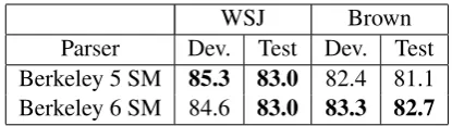
An important parameter for the Berkeley parser is the number ofsplit-merge iterationsdone dur-ing traindur-ing (cf. Petrov and Klein, 2007). The documentation suggests6is better for parsing the WSJ, while 5is better for parsing other English. We tried both. The results are shown in Table 1. We will use whichever parameterization did better
WSJ Brown
[image:4.595.312.520.61.119.2]Parser Dev. Test Dev. Test Berkeley 5 SM 85.3 83.0 82.4 81.1 Berkeley 6 SM 84.6 83.0 83.3 82.7
Table 1: Performance of the Berkeley parser on the prepositional phrase attachment task. The best scores on each data set will be our baseline.
on each data set as the baseline on that data set.3
3.5 Reduction of Open-Class Words
In all experiments, all nouns and verbs were re-placed by more general forms. If applicable, nouns were replaced by their NER label, either person,placeororganization, using the NER clas-sifier of Finkel et al. (2005). All numeral strings of two or four digits were replaced with a symbol representing year, and all other numeral strings were replaced with a symbol representingnumeric value.
A word not reduced in either of these ways was replaced by its stem using the stemmer designed by Minnen et al. (2001).4
Finally, this reduced form is paired with the cat-egory of the wordc ∈ {NOUN,VERB} to distin-guish uses of words that can either be nouns or verbs. We find that these reductions improve per-formance slightly and also reduce the size of the generative probability table.
4 A Discriminative Model from Labelled Data
4.1 The Model
As noted, we have access to one set{(xi,di)}of
labelled examples. We begin by discriminatively training two conditional models on this set.
Our model uses two types of features: i) struc-tural, and ii) lexical.
The structural features exploit two characteris-tics of prepositional phrase attachment that are of-ten noted in the literature. First, a prepositional phrase headed by the prepositionofalmost always attaches to the nearest available attachment site to its left. So, one feature fires whenever this is
3The performance of this parser depends on a random
seed used to initialize the training parser. Our6-iteration grammar was downloaded from the authors’ web site. Our
5-iteration grammar is the one that resulted from our first run of the training process.
4
not the case. Second, prepositional phrases almost never attach to pronouns. So, another feature fires whenever some prepositional phrase attaches to a pronoun.
The first model, denotedpD1(d|x;θD1), uses
these and lexical features of the form
hhead,prepi
Here,headis either a noun or a verb, andprepis a preposition. The featurehhead,prepiis active in derivation diff (a prepositional phrase headed by)prepmodifiesheadind.
Our second model,pD2(d|x;θD2), has all
fea-tures mentioned above, and also those of the form
hhead,prep,nouninsidei
Here, head and prep are as before, and nouninside is the head of the noun phrase inside
the prepositional phrase headed byprep. For example, in
[NPsalad [PPwith [NPdressing]]]
The active features are hsalad, withi and
hsalad, with, dressingi.
This latter type of feature represents straight-forward specialization of the concept used by higher-order dependencies for parsing, especially Carreras (2007), to the problem of prepositional phrases.
Our estimates ofθD1 andθD2 are arrived at
us-ing structured perceptron trainus-ing (Collins, 2002). The models trained on all examples in our training section (i.e. those of type NP and of type VP). We pick the number of perceptron training iterations for each model by maximizing performance on a held-out set, using our parameter tuning split de-scribed in§3.3. We only use feature instances that have occurred at least twice in training.
If Φ(x,d) is a feature vector characterizing
(x,d), the perceptron algorithm will output a parameter vector θDi, and the “score” assigned
to a pair (x,d) under this interpretation will be θDi ·Φ(x,d), with the predicted derivation being
thedwith the highest score (in the case of any tie, we always choose attachment to the verb).
As we have suggested, we are interested in a conditional probability ford givenx, rather than just a linear “score”. This is for use in a future section (i.e.§6). The natural way to achieve this is
WSJ Brown
Classifier Dev. Test Dev. Test pD2 (2nd-order) 87.4 86.0 84.7 83.9
pD1 (1st-order) 86.2 86.0 84.7 83.0
[image:5.595.318.518.61.132.2]Baseline 85.3 83.0 83.3 82.7
Table 2: Performance of the two discriminative classi-fiers.
to interpretθDi as the parameters for a maximum
entropy model, i.e.
pDi(d|x;θDi) =
exp{θDi ·Φ(x,d)} P
d0 exp{θD
i·Φ(x,d 0)}
Fortunately, we will see that we never need actu-ally compute the normalizing term in the denomi-nator.
4.2 Results
The performance of this model both in- and out-of-domain are shown in Table 2, along with the performance of the baseline Berkeley parser.
The results should be of interest to those inter-ested the use of lexical features for parsing. The models that use lexical features outperform the semi-lexical model of Petrov and Klein (2007). Prepositional phrase attachment may be one area where lexicalized models are especially important. We also see that the use of second-order fea-tures buys extra performance on some data sets, but not on others. A look at the dev. sets show that second-order features were active in9 of the first60 decisions in the WSJ, but in0of the first
60in Brown. We speculate that use of word senses as features, taking after Stetina and Nagao (1997), might result in better generality across domains, but leave this to future work.
5 Two Generative Models Trained on Unlabelled Data
5.1 Common Model Structure
We now want to make use of our unlabelled data,
{xj}. For this purpose, we turn to the Expectation
Maximization algorithm (Dempster et al., 1977). Thus, we will estimate generative models of the data, each of the formpG∗(x,d;θG).
It would seem impossible to expect that we could learn the structural features, e.g., that prepo-sitional phrases do not attach to pronouns from un-labelled data. Nor do we need to do this, as this constraint can be encoded with little effort. What we do want to be able to estimate from unlabelled data is the strength of lexical relationships in arbi-trary domains, which we could not hope to encode manually.
So, the question arises as to how to incorporate our knowledge of the structural constraints into the problem, and to constrain the EM process us-ing these. Probably the most powerful and general purpose way to do this would be to use one of the new variants of EM that allows the specification of expectations for feature counts, such as Ganchev et al. (2010) or Druck and McCallum (2010). In this case we could specify that, e.g., we expect the average number of times we see a prepositional phrase attach to a pronoun to be0, and the mod-ified EM process would be encouraged or forced to converge to a solution that respects this expec-tation. This strategy is very general, but also much more expensive than ordinary EM, as each E-step involves an expensive optimization problem.
Here, we get by with a simpler, and much more computationally inexpensive strategy.
The structural constraints we have made use of are very robust. In our WSJ sections2−21, of-headed PPs attach to the nearest non-pronoun to their left in about98.6%of cases. And, in99.6%
of cases, pronouns have nothing attaching to them. Thus, we are willing to take a deterministic stance: we will assign 0 probability mass to derivations that violate our structural constraints. LetAD, intuitively the set of “admissible deriva-tions,” be the set of derivations that have: i) no attachment to a pronoun, unless there is no other choice, and ii) everyof-pp attaching to its nearest available non-pronoun site, if it has one.
Let 1d∈AD be an indicator function, which is
equal to1ifd∈AD, and0otherwise. Then, the strategy is to let
pG∗(x,d) = pG∗(x,d|1d∈AD)·1d∈AD
and to estimate pG∗(x,d | 1d∈AD) from unla-belled data. The result is easily seen to be a prob-ability distribution in which all weight is given to derivations inAD.
We will look at two model structures. In both cases, the data trained on will include all examples
of type VP and NP from our GigaWord set. Ex-amples with unambiguous attachment, such as [NP
place [PP at table]], are included, so that
parame-ters chosen must maximize likelihood over these examples as well. Also note that, since the num-ber of derivations is never unmanageable, when summing over derivations, we do so exhaustively rather than use some form of dynamic program-ming such as, e.g., the inside-outside algorithm.
We will now look at two different ways to struc-ture a model forpG∗(x,d|1d∈AD).
5.2 Individual Dependent Generation
The first model uses the same lexical features as our first-order discriminative model. We model a derivation as a series of sub-events, which will be draws from a pair of random variables,
(head,prep). Intuitively, this corresponds to the eventthe phrase headed byheadgenerates a modifier headed byprep. Following the reason-ing of Collins (1999, p. 46), we imagine that each head’s final modifier is a specialSTOPsymbol.
Thus, the derivation
(6) [VPate [NPsalad] [PPwith [NPfork]]]
is modeled as the four events (eat, with), (eat, STOP), (salad, STOP), (fork, STOP).
Then, the probability of a problem-derivation pair, conditioned on1d∈AD, is estimated as
pGInd(x,d|1d∈AD;θGInd) =
Y
h∈heads(d)
Y
p∈deps(head)
pGInd(prep|head;θGInd)
Hereheads(d)is the set of head ofN P andV P phrases ind, anddeps(head)is the list of modi-fiers ofheadind, including the STOPsymbol.
Even though our unlabelled training set was large, there were still nouns and verbs seen during test that were not seen during training. Thus, we created a GENERIC head for each category (one for VERB and one for NOUN). Each time an event (head,prep) was counted, we would also count(GENERICtype(head),prep), wheretype(head) ∈ {VERB,NOUN}. Thus, the generic head represents a kind of “average head.” Then, if we needed the probability for some event
5.3 Collective Dependent Generation
The next strategy we try is to generate the collec-tion of dependents for a head head as a whole. In particular, we generate each head’smulti-setof dependents.5
In this case, if a verb has a direct object, the direct object is represented in the multi-set of the verbs modifiers. But, rather than put the word it-self, each direct object is represented by a special symbol,DO.
So, in this model, (6) is modeled as three events, (eat,{DO, with}), (salad,{}), and (fork,{}).
Then, ifdepsd(head)is the multi-set of
mod-ifiers ofheadind, our estimate of the probabil-ity of the problem-derivation pair, conditioned on 1d∈AD, is
pGCol(x,d|1d∈AD;θGCol) =
Y
head∈heads(d)
pGCol(depsd(head)|head;θGCol)
Unseen heads are handled in the same manner as in§5.2.
5.4 Initializing and Terminating the EM Process
We consider two cases for initializing the EM pro-cess. In one case, our initial guess at the posterior distribution is the uniform distribution: all deriva-tions for a givenxthat are inAD are considered equally likely, with small random perturbations to break any symmetry (we found there to be essen-tially no difference from run to run).
In the second case, we make better use of our labelled data, and begin with the conditional dis-tribution given bypD1, the model with only
first-order features, that we had estimated discrimina-tively from labelled data, i.e.
pG∗(d|x,1d∈AD;Ø) =pD1(d|x;θD1)
Given that running EM to convergence can overfit the training data, to the detriment of perfor-mance (cf., Liang and Klein (2009)), we chose to run EM for a fixed number of iterations, with the number of iterations determined using a tuning test set. We picked the number of iterations to maxi-mize performance of the best performing model (which turned out to be the collective dependent
5We also experimented with lists and sets, finding
multi-sets to work slightly better. To avoid losing the focus of this discussion, we will only discuss multi-sets.
generation initialized withpD1) on a Brown
tun-ing set, sections4-6.6The optimal number of iter-ations was found to be4.
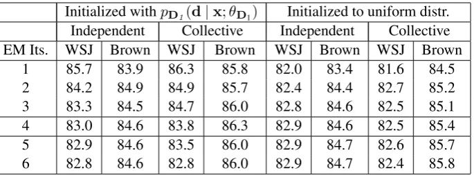
5.5 Results
The performance of these two model structures, under the two kinds of initialization methods, is shown in Table 3. Performance on the dev. test sets is plotted versus the number of iterations of the EM procedure. The fourth row is highlighted as this was determined to be the optimal number of iterations in the manner just described.
We see that the best performing method is that which generates the (multi-set of the) modifiers simultaneously, while initializing using the con-ditional distribution estimated from labelled data. It is also interesting to note that, models initial-ized withpD1 get progressively better at parsing
Brown but worse at parsing WSJ. In fact, after6
iterations, performance at parsing the WSJ is sim-ilar for both models initialized withpD1 and those
initialized with the uniform distribution. This sug-gests to us that the information that we have from our valuable labelled data is being lost, and leads us to think that it may be profitable to incorpo-rate this information more forcefully, using tech-niques for constraining EM with information, such as those of Ganchev et al. (2010) and Druck and McCallum (2010) already mentioned.
However, though the model may be “losing” in-formation relevant to parsing the WSJ, the note-worthy aspect is that it ends up being able to parse the Brown data better than our discriminatively trained parsers (both with accuracy of 84.7 on Brown dev. test), and thus makes a contribution to overall parsing accuracy.
Note that we show the performance of the vari-ous models on the development test set only here. We report results on a held-out set in the next sec-tion.
6
Initialized withpD1(d|x;θD1) Initialized to uniform distr.
Independent Collective Independent Collective EM Its. WSJ Brown WSJ Brown WSJ Brown WSJ Brown
1 85.7 83.9 86.3 85.8 82.0 83.4 81.6 84.5
2 84.2 84.9 84.9 85.7 82.4 84.4 82.7 85.2
3 83.3 84.5 84.7 86.0 82.8 84.6 82.5 85.1
4 83.0 84.6 83.8 86.3 82.9 84.6 82.5 85.4
5 82.9 84.6 83.5 86.0 82.9 84.7 82.6 85.7
[image:8.595.129.472.61.188.2]6 82.8 84.6 82.8 86.0 82.9 84.7 82.4 85.8
Table 3: Performance of the two generative models. Variables are: i) the model learned, independent vs. collective modifier generation (§5.2, 5.3), ii) the intial guess at a conditional distribution for hidden variables (§5.4), and iii) the number of iterations of EM. Score is the binary decision score (cf.§3.2).
6 A Combination of Models
6.1 The Combination
We now have two models of prepositional phrase attachment. One is estimated from labelled data, and one from unlabelled data. Each performs well in isolation. But, we find that the combination of the two in alogarithmic opinion poolframework works better than either does alone.
With roots in Bordley (1982), a logarithmic opinion pool, as defined in Smith et al. (2005), has the form
plop(d|x) = 1
Zlop
Y
α
pα(d|x)wa
In related work, Hinton (1999) describes a prod-uct of experts, i.e. multiple models trained to work together, so that an unweighted product, will be sensible. Petrov (2010) has success with the un-weighted product of the scores of several similar parsing models. Smith et al. (2005) adjust weights by maximizing the likelihood of a labelled dataset. Here, we weight the component models so as to maximize performance on a held out set. Wherei is either1or2, let
plop,i(d|x;θDi, θGCol) =
1
Zi
· pDi(d|x;θDi)
ki ·p
GCol(d|x;θGCol)
1−ki
for someki ∈[0,1]. Thatican be1or2signifies
that we will create two combinations, one forpD1
and one forpD2. TheZi are normalizing factors.
The conditional distributionpGCol(d|x;θGCol)is
obtained from the joint, in theory, by normalizing. In practice, we never actually need to compute any
normalizing factors.7
To estimate ki, we first train θD1
0 and θ D2
0
on our WSJ tuning training sections (0,1,5-22). We then useθD1
0 to estimateθ GCol
0. Finally, we
choose the value for ki that maximizes the
per-formance of the model that combines θDi 0 with
θGCol
0 on our WSJ sections 2-4, with a simple
search over values[0, .01,· · ·, .99,1]. The opti-mal values for thekiwerek1 =.70andk2 =.71.
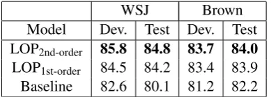
6.2 Results
Table 4 compares our two combined models against our individuals models, and our Berkeley parser baseline. We see that the combined models outperform their component models on all tasks. That is, the LOP1st-ordermodel that combinespD1
andpGCol outperforms bothpD1 andpGCol. And,
the LOP2nd-order model that combines pD2 and
pGCol outperforms bothpD2 andpGCol. This all
adds up to a significant improvement over the per-formance of the Berkeley parser. And, we see that when parsing the out-of-domain Brown data, the first-order model performs as well or slightly bet-ter than the second-order model.
Recall that we have used a new data set. In terms of past work on the Ratnaparkhi et al. (1994) data set, recall that the state-of-the-art using la-belled data alone is Stetina and Nagao (1997), with
7To see this, note that
argmax
d
f(d)
Z1
a·
g(d)
Z2
b
Z3
=argmax
d
1
Z1aZ2bZ3
f(d)ag(d)b
=argmax
d
88.1% accuracy, and with unlabelled data alone is Pantel and Lin (2000), with 84.5% accuracy. Our results compare favourably to these, though, of course, the comparison is indirect.8
Furthermore, both of these other author’s mod-els make use of semantic resources such as Word-Net and similar words lists to combat the spar-sity of combinations that occurs even in large un-labelled samples. The limited utility of second-order features based on only the stems of the nouninside suggests to us that features based on
some more general semantic concept might gen-eralize to other domains better. What is interest-ing in this regard is the strength of our first-order model, LOP1st-order, which achieves performance
approaching or passing the previous work without looking atnouninside. This suggests to us that
col-lective dependent generation is a useful technique, which can presumably be combined with the se-mantic resources of the authors just mentioned to make an even better model.
Returning to the results, while the performance on the out-of-domain Brown corpus looks very comparable to that on the WSJ for both our system and the Berkeley parser, it actually seems that the Brown corpus is somewhat “easier”, in the sense that it contains more examples that can be settled on the basis of our two fairly reliable structural heuristics.9 Table 5 shows the performance on ex-amples in which the structural heuristics do not apply. Here, we see that performance on the out-of-domain Brown corpus lags significantly behind performance on the WSJ.
Those interested in the automatic grammar dis-covery technique of the Berkeley parser will note the significant drop in performance of that parser on this subset of the data which implies that this parser had done essentially perfectly in cases where our structural heuristics did apply, meaning it must havelearnedequivalent heuristics to those that we encoded by hand, which is noteworthy.
Finally, though we have so far reported only the binary decision score (cf. §3.2) for each deriva-tion, Table 6 shows a more general score: the percentage of correct attachments in any example
8While both the Ratnaparkhi et al. (1994) test set and our
WSJ test set are from the essentially the same material, they are not exactly the same examples, as the Treebank has un-dergone reordering.
9On WSJ sections0,1,22-24, structural features fire in
33.8%of examples, while on Brown sections0-2,7-9 struc-tural features fire in46.0%of examples.
WSJ Brown
Model Dev. Test Dev. Test pGCol (4 EM its.) 83.8 81.6 86.3 85.4
LOP2nd-order 88.9 86.9 86.4 86.2
pD2 (2nd-order) 87.4 86.0 84.7 83.9
LOP1st-order 87.5 86.6 86.6 86.2
pD1 (1st-order) 86.2 86.0 84.7 83.0
[image:9.595.308.525.62.173.2]Baseline 85.3 83.0 83.3 82.7
Table 4: Performance of the combined model. Score is the binary decision score (cf.§3.2).
WSJ Brown
Model Dev. Test Dev. Test LOP2nd-order 84.1 80.3 76.0 76.2
LOP1st-order 82.3 79.8 76.1 76.3
[image:9.595.317.515.216.288.2]Baseline 78.7 74.4 70.0 69.0
Table 5: Performance of the combined model on exam-ples that cannot be settled by our two structural con-straints. I.e., examples where i) the preposition is not of, and ii) the direct object is not a pronoun. Score is the binary decision score (cf.§3.2)
(whether headed by noun or verb) in which more than one attachment was possible. Here, we see that the general problem is, as one would expect, harder than the binary decision problem.
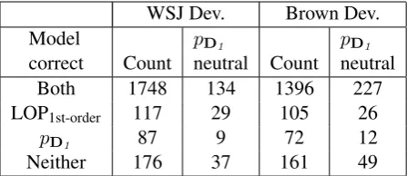
6.3 Analysis: What does Unlabelled Data Change?
At this point, we ask what difference the unla-belled data makes. To answer this question, we consider the nature of the disagreements between the pD1 itself, and the LOP1st-order model that
mixespD1 withpGCol.
In Table 7, the Countcolumn shows the num-ber of agreements and disagreements on the de-velopment test sets. One possible outcome would have been few disagreements between models and that each of these would be won by the combined model. In fact, a significant number of
disagree-WSJ Brown
Model Dev. Test Dev. Test LOP2nd-order 85.8 84.8 83.7 84.0
LOP1st-order 84.5 84.2 83.4 83.9
Baseline 82.6 80.1 81.2 82.2
[image:9.595.320.515.637.707.2]WSJ Dev. Brown Dev. Model
correct Count pD1
neutral Count pD1
neutral
Both 1748 134 1396 227
LOP1st-order 117 29 105 26
pD1 87 9 72 12
[image:10.595.72.296.62.159.2]Neither 176 37 161 49
Table 7: Analysis of the agreements and disagreements between the first-order discriminative classifier, pD1, and the combined model, LOP1st-order. The second row
describes examples where LOP1st-orderwas correct but pD1 was wrong, and the third row describes the con-verse situation. TheCountcolumn gives the number of examples in each category. The pD1neutral col-umn gives the number of examples in each category in which no features in thepD1model were active (the strategy is to pick attachment to verb in this case).
ments go each way, but the large majority are won by the combined model.
ThepD1 neutralcategory counts the number of
times that none ofpD1’s features fire. These are
the examples in whichpD1 has no opinion
what-soever, and so the combined model should have an advantage, if the unlabelled data is contribut-ing useful information. We see that this is indeed the case. When no features fire forpD1, the
strat-egy, as noted, is to choose attachment to the verb, which should still lead to a large number of cor-rect responses. Thus, it makes sense that some disagreements are won by pD1, even when none
of its features fire.
7 Conclusion and Future Work
We have shown that supervised techniques based on lexical dependency parsing outperform the semi-lexicalized strategy of Petrov and Klein (2007).
We have demonstrated that a properly chosen pair of models, one trained discriminatively from labelled data, and one trained generatively from unlabelled data, can be combined in a product model to yield a model better than either is alone. We have shown that, when learning from unla-belled data, it may be preferable to generate de-pendents collectively.
Finally, we have introduced a pair of models which we think will be interesting to combine us-ing the new methods for constrainus-ing EM, e.g., a la Ganchev et al. (2010) or Druck and McCallum (2010).
Acknowledgements
We thank Ioannis Konstas, Micha Elsner, and the reviewers for helpful suggestions. This work was supported by the Scottish Informatics and Com-puter Science Alliance and the ERC Advanced Fellowship 249520 GRAMPLUS.
References
Michaela Atterer and Hinrich Sch¨utze. 2007. Prepositional phrase attachment without ora-cles. Computational Linguistics, 33(4):469– 476.
R. F. Bordley. 1982. A multiplicative formula for aggregating probability assessments. Manage-ment Science, 28:1137–1148.
Eric Brill and Philip Resnik. 1994. A rule-based approach to prepositional phrase attachment disambiguation. In COLING, pages 1198– 1204.
Xavier Carreras. 2007. Experiments with a higher-order projective dependency parser. In Proceedings of the CoNLL Shared Task Session of EMNLP-CoNLL 2007, pages 957–961.
Michael Collins and James Brooks. 1995. Prepo-sitional phrase attachment through a backed-off model. CoRR.
Michael Collins. 1999. Head-Driven Statistical Models for Natural Language Parsing. Ph.D. thesis, University of Pennsylvania.
Michael Collins. 2002. Discriminative train-ing methods for hidden Markov models: theory and experiments with perceptron algorithms. In EMNLP, pages 1–8, Stroudsburg, PA, USA. As-sociation for Computational Linguistics.
A. P. Dempster, N. M. Laird, and D. B. Rubin. 1977. Maximum likelihood from incomplete data via the EM algorithm. Journal of the Royal Statistical Society, B, 39.
Jenny Rose Finkel, Trond Grenager, and Christo-pher D. Manning. 2005. Incorporating non-local information into information extraction systems by Gibbs sampling. InACL.
Kuzman Ganchev, Jo˜ao Grac¸a, Jennifer Gillenwa-ter, and Ben Taskar. 2010. Posterior regulariza-tion for structured latent variable models. Jour-nal of Machine Learning Research, 11:2001– 2049.
Daniel Gildea. 2001. Corpus variation and parser performance. In Lillian Lee and Donna Har-man, editors, Proceedings of the 2001 Confer-ence on Empirical Methods in Natural Lan-guage Processing, EMNLP ’01, pages 167– 202, Stroudsburg. Association for Computa-tional Linguistics.
David Graff, Junbo Kong, Ke Chen, and Kazuaki Maeda. 2005. English Gigaword Second Edi-tion. Linguistic Data Consortium: Philadel-phia.
Donald Hindle and Mats Rooth. 1991. Structural ambiguity and lexical relations. In ACL’91, pages 229–236.
Geoffrey Hinton. 1999. Product of experts. In ICANN.
Percy Liang and Dan Klein. 2009. Online em for unsupervised models. In HLT-NAACL, pages 611–619.
Mitchell P. Marcus, Beatrice Santorini, and Mary Ann Marcinkiewicz. 1993. Build-ing a large annotated corpus of English: The Penn Treebank. Computational Linguistics, 19(2):313–330.
Guido Minnen, John Carroll, and Darren Pearce. 2001. Applied morphological processing of en-glish. Nat. Lang. Eng., 7:207–223, September.
Patrick Pantel and Dekang Lin. 2000. An un-supervised approach to prepositional phrase at-tachment using contextually similar words. In ACL.
Slav Petrov and Dan Klein. 2007. Improved infer-ence for unlexicalized parsing. InHLT-NAACL, pages 404–411.
Slav Petrov. 2010. Products of random latent vari-able grammars. InHLT-NAACL, pages 19–27.
Adwait Ratnaparkhi, Jeffrey C. Reynar, and Salim Roukos. 1994. A maximum entropy model for prepositional phrase attachment. InHLT.
Adwait Ratnaparkhi. 1998. Statistical models for unsupervised prepositional phrase attachement. InCOLING-ACL, pages 1079–1085.
Andrew Smith, Trevor Cohn, and Miles Osborne. 2005. Logarithmic opinion pools for condi-tional random fields. InACL.
J. Stetina and M. Nagao. 1997. Corpus based pp attachment ambiguity resolution with a seman-tic dictionary. InNatural Language Processing Pacific Rim Symposium.
Kristina Toutanova, Christopher D. Manning, and Andrew Y. Ng. 2004. Learning random walk models for inducing word dependency distribu-tions. InICML.
Martin Volk. 2002. Combining unsupervised and supervised methods for pp attachment disam-biguation. In Proceedings of the 19th interna-tional conference on Computainterna-tional linguistics - Volume 1, COLING ’02, pages 1–7, Strouds-burg, PA, USA. Association for Computational Linguistics.
Appendix A: Extracting Examples from Gold Trees
In this section, we describe the functional program used to extract examples from gold trees.
A base noun phrase is phrase labelled NP, which does not dominate any other phrases. A base noun phrase is identified with its head-word. Head words are found using the Java reimplemen-tation of Collins (1999) head-finder in the Stanford NLP API.
Noun phrase examples extracted are those that match
[S. . . [NP1 BaseNPH(prep baseNP)i
∗. . . ] . . . ]
NP1 must be immediately dominated by an S,
baseNPHmust be the left-most descendant of NP1,
and all (prep baseNP)i substrings must be
domi-nated by NP1as well.
Verb phrase examples are those that match
[VP1 verbH(PRT) (ADVP) (baseNP) (prep baseNP)i
+. . . ]
VP1 can occur in any environment. If there is a