Can more be less? An experimental test of the resource curse

Munich Personal RePEc Archive

Can more be less? An experimental test

of the resource curse

Al-Ubaydli, Omar and McCabe, Kevin and Twieg, Peter

31 March 2014

1

Can more be less? An experimental test of the resource curse

Omar Al-Ubaydli, Kevin McCabe and Peter Twieg1

March 2014

A

Several scholars have argued that abundant natural resources can be harmful to economic performance under bad institutions and helpful when institutions are good. These arguments have either been theoretical or based on naturally-occurring variation in natural resource wealth. We test this theory using a laboratory experiment to reap the benefits of randomized control. We conduct this experiment in a virtual world (Second LifeTM) to make institutions more visceral. We find support for the theory.

JEL codes: D72, D74, O13, Q34

Keywords: resource curse; institutions; economic development

I

Can a nation ever find itself regretting discovering some of its natural resources? Many have posed this question after witnessing the hardship in resource-rich countries such as Libya or Iraq. Sachs and Warner (1995) and a large literature have presented considerable evidence that natural resources can indeed be a curse for a variety of reasons, including diminished income growth, lower income, or adversely affected institutions (Ross 2001, Frankel 2010).

The focus of our study is the recently proposed, refined version of the resource curse, whereby the negative consequences of natural resources are restricted to economies with weak institutions (Torvik 2002, Acemoglu et al. 2004, Robinson et al. 2005, Acemoglu and Robinson 2006, Hodler 2006, Mehlum et al. 2006, Olsson 2006, 2007, Bulte and Damania 2008, Vicente 2010, Al-Ubaydli 2011). We test a modified version of the Torvik (2002) model in a laboratory virtual world experiment. Players allocate their labor between production, which is positive-sum, and rent-seeking in the natural resource sector, which is zero-sum. If players play the symmetric Nash equilibrium, then resource booms attract labor away from the productive sector towards

1 _{We wish to thank Noel Johnson, Rebecca Morton, Jim Murphy, Joshua Tucker and several anonymous reviewers}

2

rent-seeking to such a degree that aggregate income decreases—the resource curse. However, if players can establish institutions that promote cooperation (North 1990, North et al. 2009), they can realize the benefits of a resource boom.

We vary two factors: natural resource income; and the players’ ability to communicate and monitor each other—a key determinant of the quality of institutions. We find strong support for the prediction that the resource curse arises only in economies with weak institutions. In general, we find evidence of a mild version of the resource curse, whereby groups with weak institutions tend to squander all the benefits of a resource boom, and may even be harmed by it.

Previous empirical studies have failed to obtain exogenous variation in both of these explanatory variables, instead relying on potentially endogenous, naturally occurring variation (studies such as Tsui 2009 and Acemoglu et al. 2001 rely on plausibly exogenous variation but do not use it to study economic performance; also see Compton et al. 2010). In fact, the empirical debate over how to best handle endogeneity has led to Alexeev and Conrad (2009) questioning whether the aggregate data even support the existence of a resource curse.

This paper has two main contributions. First, by using a laboratory experiment, we can implement randomized control in the explanatory variables of interest, guaranteeing exogenous variation (see Leibbrandt and Lynham 2013 for a complementary experimental investigation). Second, by allowing players to interact in a visceral environment (the Second LifeTM _virtual

world), we can more fully explore the nuances of strong vs. weak institutions. By providing clean evidence of the refined, institutions-mediated model of the resource curse, our paper represents a significant step in our understanding of the economic impact of natural resources.

M

The Torvik (2002) model is well-suited for theoretically exploring the effect of natural resources on societal welfare. However, in its original form, the large number of players and the environment’s complexity render it ill-suited for a laboratory experiment. We modify the model, drawing heavily upon Morgan and Sefton (2000) and the rent-dissipation literature (Tullock 1980, Walker et al. 1990, Baye et al. 1994, Nti 1997, Potters et al. 1998, Knapp and Murphy 2010). More generally, we are only testing one of several distinct causal mechanisms proposed by resource curse scholars. We restrict our attention to the institutions-mediated version of the resource curse to sharpen our focus and because of its suitability for laboratory experimentation.

The economy is populated by identical players, indexed by 𝑖 ∈ {1,2, … , 𝑛}, interacting for one period. Each has one unit of time to allocate between rent-seeking pursuit of the natural resource

(𝑥𝑖) and production (1 − 𝑥𝑖). The economy-wide income from the natural resource is 𝑅 > 0,

3

0, then each gets (1/𝑛)𝑅.) This implies a negative externality to allocating resources to the natural resource sector: 𝑖 can only increase her share by decreasing that of others.

Production has a positive externality: for each unit of time that 𝑖 allocates to production, she receives 𝛼 > 0 and each player 𝑗 ≠ 𝑖 receives 𝛽 > 0. Thus 𝑖’s payoff is:

𝑦𝑖 = 𝛼(1 − 𝑥𝑖) + 𝛽 ∑(1 − 𝑥𝑗) 𝑗≠𝑖

+ 𝑅_{∑ 𝑥}𝑥𝑖

𝑗 𝑗

Analogous results can be obtained by eliminating the positive externality in production and having a stronger negative externality in the natural resource sector, or by having increasing returns in the productive sector, similar to Torvik. (See the appendix for more on this.)

Why should we expect strong negative externalities in the natural resource sector? Economists have long regarded a substantial proportion of natural resource income to be economic rent (Sachs and Warner 1995), which invites zero-sum rent-seeking behavior (Tullock 1980, Nti 1997). The rent-seeking can become wasteful socially as the groups in control of the rent erect barriers to secure their position (Auty 2001), and the conflict can become violent (Frankel 2010). Our precise specification is motivated by a desire to keep payoffs as simple as possible (for the purposes of running an experiment) subject to retaining the spirit of Torvik (2002).

EQUILIBRIUM

Let 𝑌 = ∑ 𝑦_{𝑖 𝑖} denote GDP. Each player chooses 𝑥_𝑖 ∈ [0,1] to maximize 𝑦_𝑖 given

(𝑥1, … , 𝑥𝑖−1, 𝑥𝑖+1, … , 𝑥𝑛). The maximand is smooth and strictly concave; assuming an interior

solution, the unique symmetric Nash equilibrium is (see the appendix for all proofs):

𝑥𝑁𝐸 ₌ (𝑛 − 1)𝑅

𝛼𝑛2 , 𝑌𝑁𝐸 =

1

𝛼𝑛((𝛼 − 𝛽(𝑛 − 1)2)𝑅 + 𝛼2𝑛2+ 𝛼𝛽(𝑛 − 1)𝑛2)

In contrast, the symmetric Pareto efficient outcome is:

𝑥𝑃𝐸 _{= 0, 𝑌}𝑃𝐸 _{= (𝛼 + 𝛽(𝑛 − 1))𝑛 + 𝑅 > 𝑌}𝑁𝐸

We refer to players who play the Nash equilibrium as non-cooperative players, players who play the Pareto efficient equilibrium as cooperative players, and an increase in 𝑅 as a resource boom.

Proposition 1: In response to a resource boom:

4

Resource booms increase the marginal private return to rent-seeking, but the marginal social return to rent-seeking is always zero since rent-seeking is purely redistributive. The marginal private and social costs to rent-seeking are both positive and unaffected by 𝑅.

Proposition 2: In response to a resource boom:

a) For a sufficiently large 𝛽, GDP in a non-cooperative economy will fall; 𝜕𝑌𝑁𝐸/𝜕𝑅 < 0 b) GDP in a cooperative economy always increases one-to-one; 𝜕𝑌𝑃𝐸/𝜕𝑅 = 1 > 0

The marginal social cost to rent-seeking, 𝛼 + (𝑛 − 1)𝛽, exceeds the marginal private cost, 𝛼. When 𝛽 is sufficiently large, the increased rent-seeking brought about by a resource boom actually decreases GDP in a non-cooperative economy as too many resources are shifted from the positive-sum production sector to the zero-sum natural resource sector. In contrast, a cooperative economy reaps the full benefits of a resource boom.

Our goal is to investigate the possibility that an economy regrets a resource boom. The above

version of the resource curse uses levels of GDP rather than, say, GDP’s growth rate. We chose levels to simplify the theoretical exposition and to facilitate laboratory testing; however the thrust of the argument in Torvik (2002)—and hence our argument—does not depend upon any particular outcome variable.

If this game is repeated finitely with period-by-period payoff information, by backward induction, the symmetric Nash equilibrium, efficient play, and all the predictions are retained. The symmetric Nash equilibrium also remains an equilibrium even if the game is repeated infinitely.

INSTITUTIONS

The model’s predictions hinge upon whether the players play cooperatively vs. non -cooperatively. Torvik (2002), Hodler (2006), Mehlum et al. (2006), Olsson (2006, 2007), Bulte and Damania (2008) and Al-Ubaydli (2011) argue that this is determined by the quality of institutions (North 1990). Other models that predict an ambiguous effect of natural resources are Acemoglu et al. (2004), Robinson et al. (2005), Acemoglu and Robinson (2006) and Andersen and Aslaksen (2008), but they explore different mechanisms.

5

How do good institutions come about? We will not tackle this sizeable topic comprehensively in this paper (Acemoglu and Robinson 2006, Greif 2006). For the purposes of a laboratory experiment, a good departure point is Ostrom (2000), which emphasizes cooperation and coordination. She concisely summarizes her findings in the form of several design principles:

 Clear boundary rules (Kimbrough et al. 2009, McCabe et al. 2011)

 Clear usage rules

 The individuals affected by the rules participate in rule-making

 The stakeholders select and hold accountable the monitors

 Graduated sanctions for rule-violation

 Access to conflict-resolution arenas

A common thread is the need for communication channels and monitoring mechanisms.

Ostrom’s fieldwork is complemented by a large experimental literature on the benefits of communication to cooperation and coordination (Cooper et al. 1992, Burton and Sefton 2001, Duffy and Feltovich 2002, Charness and Grosskopf 2004, Brandts and Cooper 2005, Blume and Ortmann 2007).

For the purposes of the present model, we can think of good institutions as being those that increase the likelihood of the players playing cooperatively. Good institutions include a clear allocation of property rights, which decreases the usefulness of violence and lobbying as a means of securing a larger share of the pie. They also include a strong sense of community and mutual affection among stakeholders, which limits selfish rent-seeking. Beyond this, they include punishment mechanisms that can further deter rent-seeking. In the appendix, we formally integrate institutions into our model, and explain how communication channels can bring about good institutions. For now, in the interests of brevity, we focus on the result.

Proposition 3: In repeated play, cooperative play is more likely the greater the opportunity to communicate and monitor.

E

D

Procedure: Each session has 12 players and proceeds in the following manner.

 Virtual world training

 Round 1: Play the main game in groups of 4 for 15 minutes with natural resource income

𝑅 = 𝑟1.

6

 Round 3: Reassigned to new groups of 4 and play the main game for 15 minutes with

𝑅 = 𝑟2.

To minimize noise, we made the experiment long enough to allow players to explore their environment and experiment with strategies. Players were anonymously assigned unique in-game names that they retained throughout the session. We reassigned groups to minimize the reputational transfer across rounds.

Parameters: Players played a continuous time version of the game in our model under a neutral

frame (e.g., “Activity X”instead of “production”), and with the following parameter values.

 Group size 𝑛 = 4

 Private production return 𝛼 = $800/minute

 External production return 𝛽 = $500/minute

 Natural resource income: high 𝑟_𝐻 = $4,000/minute and low 𝑟_𝐿 = $1,200/minute

 The support of 𝑥 is transformed to integers in the range [0,100]

𝑥𝐿𝑁𝐸 = 28, 1_𝑛𝑌𝐿𝑁𝐸 = $1,953/𝑚𝑖𝑛, _𝑛1𝑌𝐿𝑃𝐸 = $2,600/𝑚𝑖𝑛

𝑥𝐻𝑁𝐸 = 94, 1_𝑛𝑌𝐻𝑁𝐸 = $1,144/𝑚𝑖𝑛, _𝑛1𝑌𝐻𝑃𝐸 = $3,300/𝑚𝑖𝑛

Under non-cooperative play, the resource curse will materialize (𝑌_𝐿𝑁𝐸 > 𝑌_𝐻𝑁𝐸). Under cooperative play, GDP per capita should increase by $700/min (27%) when 𝑅 = 𝑟_𝐻. In each session, we randomly assigned 𝑟₁= 𝑟_𝐻, 𝑟₂ = 𝑟_𝐿 or the reverse. At the start, players learn 𝑟₁ and they are informed that it may change, with any change being preceded by an announcement.

Information: Players receive continuous information about their payoff broken down into: the amount they are earning from their production; from others’ production; and from rent-seeking. This allows players to identify when others are rent-seeking without knowing the rent-seeker’s identity. To facilitate payoff calculations, players are continuously told how their payoff will change if they allocate one more/less unit to rent-seeking. In principle, making this information so saliently available could induce players to change their rent-seeking with higher frequency than would be rational (especially in the no-comms treatment below, where there is less for players to do during a session).

We were unconcerned by this prospect because optimal rent-seeking was dependent on the choices of other players, which were themselves changing in real time, and so technically, it was optimal for players to regularly change their rent-seeking. Given the ample time afforded for experimentation, subjects will plausibly have inferred the importance of continually fine-tuning their rent-seeking.

7

variation, with half the sessions starting with 𝑟₁ = 𝑟_𝐻 = $4,000 and the other half starting with

𝑟1= 𝑟𝐿= $1200.

The second explanatory variable is the opportunity to communicate and monitor. Our baseline treatment is no comms, where players have no way of communicating. This corresponds to the poorest institutions and is designed to induce non-cooperative play.

Our second treatment is partial comms. Players can communicate with fellow group members via a live chat interface for 2 minutes prior to the start of each round. It is common knowledge that once the round actually starts, the players will revert to the conditions in the baseline. This gives players an opportunity to establish some informal norms and to discuss optimal strategies. This treatment corresponds to (the opportunity for) an intermediate quality of institutions and is more likely to result in cooperative play than the no comms treatment.

Our third treatment is full comms. In addition to the pre-round communication of the partial comms treatment, players can chat throughout the 15 minutes of the round. Each player also has the ability to intermittently monitor the rent-seeking activities of 2 out of her 3 fellow group members. This gives players much more information on the distribution of rent-seeking, allows them to administer targeted verbal sanctions, helps create a sense of community and mutual affection, and provides a forum for discussing the best response to the natural resource shock in the middle of round 2. This corresponds to (the opportunity for) high quality institutions and the best chance of cooperative play.

We chose not to run the additional treatments necessary to parse the role of communication vis-à-vis monitoring because it was not relevant to our main goal: demonstrating that under sufficiently poor institutions, the resource curse appears, and that under sufficiently good institutions, the resource curse is absent. The precise configuration of institutions at which the resource curse pendulum swings is a topic for future research.

Virtual world environment: Each session was conducted using the virtual world of Second LifeTM _{(Chesney et al. 2009, Fiedler et. al 2011, Atlas and Putterman 2011). Second Life}TM

places individual users into the role of controlling a graphical avatar and navigating and interacting with a three-dimensional spatial environment (Figure 1).

Second LifeTM was employed in this study in order to naturalistically implement many of the features outlined in Ostrom (2000). It is possible to study how communication and monitoring interact with the institutions-mediated resource curse in an environment devoid of the visceral, visual elements inherent in Second LifeTM_{, e.g., using zTree (Fischbacher 2007), though to the}

best of our knowledge, no such experiment has been done.

8

the cooperative institutions that can overcome natural resource management problems (Charness et al. 2007, Charness and Gneezy 2008).

The spatial layout of the experimental environment is depicted in Figure 2. Each group interacted within a separate copy of this environment. It is divided into a central area in which subject training occurs prior to the first experimental round, and four outer areas each inhabited by one subject. Each subject is able to view its two adjacent neighbors, and can check on these

neighbors’ rent-seeking at various times depending on the treatment. Only one neighbor can be effectively monitored at a time, however, as subjects must travel from one side of their area to the other in order to monitor their other neighbor (this takes approximately 15 seconds).

This monitoring process is made especially salient via the fact that it not only involves the conveyance of information about rent-seeking behavior, but also visual contact between subject avatars; previous studies have demonstrated the potential significance of visceral, visual cues of monitoring to cooperative decision-making (Bateson et al. 2006). Furthermore, the ability to monitor only one neighbor at a time allowed for well-organized groups to devise collective monitoring strategies—in one group in particular it was suggested that each subject constantly monitor the his or her left-hand neighbor to ensure that each subject was constantly monitoring (and being monitored by) another subject.

Even in sessions where the monitoring and communication options of subjects were limited, subjects would extensively move around and explore their respective areas. Furthermore, this movement ability afforded subjects a rudimentary capability for communication insofar as movement patterns could be used to communicate information to neighbors. For example, it was

common for subjects to approach each other and mimic each other’s movement patterns, perhaps as a sort of pro-social display (Lakin et al. 2003). After one round in the partial comms

treatment, one subject commented that “i [sic] am pretty sure i [physically interacted]2 with a fellow avatar last round through a transparent fence.”

Rent-seeking is selected using the heads-up display (HUD) depicted in the top-left corner of Figure 1. The HUD also displays several additional pieces of information described above (absent in Figure 1 because the screenshot is from training).

RESEARCH HYPOTHESES

Our data permit us to examine the effect of a resource boom and a resource bust. For brevity, we formulate our hypotheses only in terms of booms.

9

Prediction 1: In response to a resource boom:

a) Under no comms, rent-seeking will increase b) Under full comms, rent-seeking will be unchanged

c) The increase in rent-seeking will be larger in no comms vs. partial comms, and in partial comms vs. full comms

Prediction 2: In response to a resource boom:

a) Under no comms, GDP will decrease

b) Under full comms, GDP will increase one-to-one

c) The increase in GDP will be larger in full comms vs. partial comms, and in partial comms vs. no comms

Studies in the rent dissipation literature have presented data collected from similar environments. Our study differs in that we examine the comparative statics of the size of the prize, and we consider the relationship between rent seeking and social welfare, and how it is mediated by institutions.

R

We ran 12 sessions in 2011. Sessions took place in the George Mason University Krasnow Institute laboratory. Sessions took 2 hours and average earnings were $25.

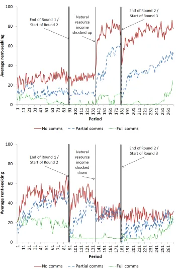
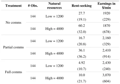
We collected data every 10 seconds. Table 1 contains the main descriptive statistics where the averages are across players and time. Figure 3 gives us a sense of the overall dynamics of rent-seeking averaging across players in each treatment.

Rent-seeking is low at the start of a round because its default value is 0. Each panel of Figure 3 supports our main hypotheses based on within variation: in the absence of communication (solid line), when natural resource income is higher, so too is rent-seeking; when communication is permitted (dotted line), rent-seeking is low and unresponsive to natural resource income. Comparing the two panels of Figure 3 also supports our main hypotheses based on between variation. However the panels of Figure 3 are based on averages and they conceal variation around the mean, to which we turn our attention now.

10

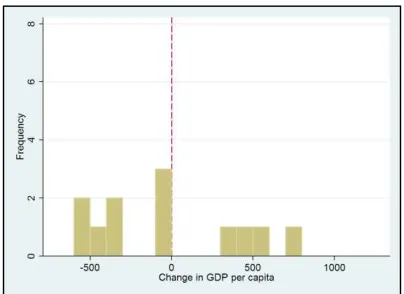
For example, according to Figure 4b, in the partial comms treatment, 8 out of 12 groups had a higher GDP per capita when 𝑅 = $4,000 than when 𝑅 = $1,200. In all treatments, if rent-seeking does not change in response to a resource boom, then GDP per capita should increase by $700. Some groups experience a greater increase than $700 because they decrease their rent-seeking in response to a resource boom. We will further discuss Table 1 and Figures 3 and 4 below in our formal results.

DATA STRUCTURE AND EMPIRICAL STRATEGY

We construct six observations per player per session by averaging each player’s 45 minutes of

data to 2 observations per player per round: 1 for the first 7½ minutes and 1 for the last 7½ minutes. Let 𝑡 ∈ {1,2, … ,6} denote the period; see Table 2. (See the appendix for a fuller discussion, including the alternatives.)

Our main dependent variables are rent-seeking, 𝑥_𝑖𝑡, and earnings, 𝑦_𝑖𝑡; 𝑖 denotes player across all sessions, i.e., 𝑖 ∈ {1,2, … ,144}. 𝐹_𝑖𝑗 is a player fixed effect that takes the value 1 when 𝑖 = 𝑗 and 0 otherwise. 𝑇_𝑡𝑠 is a time fixed effect that takes the value 1 when 𝑡 = 𝑠 and 0 otherwise. 𝑔(𝑖𝑡) is a function denoting which of the 108 groups 𝑖 finds herself in period 𝑡.

Let 𝐻_𝑖𝑡 be a dummy variable that takes the value 1 when 𝑅 = $4,000 and 0 when 𝑅 = $1,200. Let 𝐷_𝑖𝑡𝑃𝑎𝑟𝑡𝑖𝑎𝑙 be a treatment dummy for partial comms, and let 𝐷_𝑖𝑡𝐹𝑢𝑙𝑙 be a treatment dummy for full comms. We estimate the following econometric models.

𝑥𝑖𝑡 = 𝑎 + 𝑏𝐻𝐻𝑖𝑡+ 𝑏𝐼𝑛𝑡𝑃𝑎𝑟𝑡𝑖𝑎𝑙𝐻𝑖𝑡𝐷𝑖𝑡𝑃𝑎𝑟𝑡𝑖𝑎𝑙+ 𝑏𝐼𝑛𝑡𝐹𝑢𝑙𝑙𝐻𝑖𝑡𝐷𝑖𝑡𝐹𝑢𝑙𝑙+ ∑ 𝑏𝐹𝑗𝐹𝑖𝑗 144

𝑗=2

+ ∑ 𝑏𝑇𝑠𝑇𝑡𝑠 6

𝑠=2

+ 𝑢𝑔(𝑖𝑡)+ 𝜀𝑖𝑡

𝑦𝑖𝑡 = 𝑎 + 𝑏𝐻𝐻𝑖𝑡+ 𝑏𝐼𝑛𝑡𝑃𝑎𝑟𝑡𝑖𝑎𝑙𝐻𝑖𝑡𝐷𝑖𝑡𝑃𝑎𝑟𝑡𝑖𝑎𝑙 + 𝑏𝐼𝑛𝑡𝐹𝑢𝑙𝑙𝐻𝑖𝑡𝐷𝑖𝑡𝐹𝑢𝑙𝑙+ ∑ 𝑏𝐹𝑗𝐹𝑖𝑗 144

𝑗=2

+ ∑ 𝑏𝑇𝑠𝑇𝑡𝑠 6

𝑠=2

+ 𝑢𝑔(𝑖𝑡)+ 𝜀𝑖𝑡

𝜀𝑖𝑡 is a white noise error term and 𝑢𝑔(𝑖𝑡) is a group cluster to capture correlation between

decisions within a group. The player fixed effect is included to correct for within-player correlation. We exclude communication treatment variables because we include player fixed effects.

MAIN RESULTS

Result 1a: Under no comms, rent-seeking increases in response to a resource boom.

11

Result 1b: Under full comms, rent-seeking slightly increases in response to a resource boom.

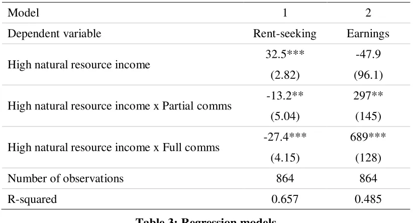
Table 2 and Model 1 in Table 3 confirm that under full comms, per capita rent-seeking increases by 5.1 (p < 0.1 using a Wald test), which is economically quite small (less than half a standard deviation). (In Model 1 of Table 3, the treatment effect is obtained by summing the coefficient

on ‘High natural resource income’ with the coefficient on ‘High natural resource income x Full

comms’.) Both pre- and post-resource boom, rent-seeking on average does not exceed 10 (out of a possible 100); overall, rent-seeking is very low under full comms.

The chat transcripts reflect the players’ success in limiting rent-seeking (we hired research

assistants who were blind to the experiment’s goal and its treatments to classify chat statements;

to ensure accurate classification, we used multiple research assistants for each of the approximately 4,500 messages exchanged in the experiments). In the two minutes prior to the start of each round, over 6% of the 640 messages exchanged by players were explicit attempts at coordinating on zero rent-seeking (and many of the remaining messages were expressions of affirmation and so the figure 6% is a substantial understatement), e.g., “Lets [sic] go all X”,

“everyone press 0 in y” and “Do what’s best for everyone and dont [sic] increase Y”. (In the experiment, production was labeled ‘Activity X’ and rent-seeking was labeled ‘Activity Y’.) In line with Ostrom (2000), successful avoidance of rent-seeking was down to a combination of overt coordination, monitoring, and sanctions. In the 36 groups in the full comms sessions, monitoring stations were used 1099 times (2.5 times per player per round). There were 18 occasions where one player explicitly and correctly accused another player of selfishly rent-seeking. If this number seems low, it is because most accusations were not directed at individual

players; more often they were of the form “someone is putting tokens in Y!!!” or “stop cheating!!!”. The (correctly) accused’s subsequent level of rent-seeking almost always went down in response to the accusation (p < 2% level using a Wilcoxon paired-values test).

Accusations were typically aggressive in tone and constituted verbal sanctions, e.g., “QUIT BEING GREEDY!!!!!!!!”.

Though harder to quantify, chat transcripts clearly reflected some groups’ success in forging a

sense of community and shared goals, which presumably helped limit rent-seeking.

Result 1c: The increase in rent-seeking in response to a resource boom is larger in no comms vs. partial comms, and in partial comms vs. full comms.

12

Similar to the full comms sessions, players in the partial comms sessions took advantage of the (limited) opportunity to chat: 8% of the 577 messages constituted an explicit attempt to coordinate on zero rent-seeking.

Result 2a: Under no comms, on average, GDP per capita does not change in response to a resource boom. However there is substantial likelihood that it decreases.

Table 1 and Model 2 in Table 3 confirm that under no comms, per capita GDP decreases by $48 (p = 0.6), which is statistically and economically insignificant (below a quarter of a standard deviation). Thus on average, we have a mild version of the resource curse, whereby most groups simply do not gain from a resource boom (when they should be gaining $700 per capita).

However if we look at Figure 4a, we can see that 8 out of 12 groups suffered a decrease in GDP per capita, and for 5 of them, this decrease was around $500 per capita, which exceeds a standard deviation in size—a veritable curse. In aggregate, their cursedness is masked by the high success of 4 groups in fully reaping the benefits of a resource boom.

Result 2b: Under full comms, GDP per capita increases one-to-one in response to a resource boom.

Table 1 and Model 2 in Table 3 confirm that under full comms, per capita GDP increases by $641 (p < 0.01), which is almost the predicted $700. A Wald test fails to reject its equality to $700 (p = 0.49). In Figure 4c, we can see that 11 out of 12 groups improve their GDP per capita as a result of a resource boom. Under full comms, resources are anything but a curse.

Result 2c: The increase in GDP in response to a resource boom is larger in full comms vs. partial comms, and in partial comms vs. no comms.

Table 1 and Model 2 in Table 3 confirm that under partial comms, per capita GDP increases by $250, which is above the estimated increase under no comms and smaller than that under full comms. Using Wald tests, we can reject the hypotheses that it is equal to either (p < 0.01). The intermediacy of the partial comms treatment is reflected in Figure 4b, where large gains and losses can be seen in response to resource booms.

In the appendix, we demonstrate the robustness of our results to changing various aspects of the data structure and estimation technique, as well as some ancillary results concerning how close

the players’ actions are to a Nash equilibrium.

C

13

booms can be completely squandered and that on occasion, more can indeed be less. The key ingredient in ensuring the rigorousness of our evidence is our deployment of randomized control,

in contrast to the literature’s typical dependence on observational data. Our data also support the institutions-mediated version of the resource curse, whereby groups with good institutions reap the full benefits of resource booms.

While we could have explored the same questions in a conventional laboratory experiment (Leibbrandt and Lynham 2013), we chose to allow participants to interact in a three-dimensional virtual world. We did this to more accurately capture the features of good institutions that Ostrom (2000) argued characterized successful natural resource management, while retaining the simplicity necessary to test our model.

Historians (Engerman and Sokoloff 1997) and economists (Acemoglu et al. 2001) have offered important insights into how natural resources interact with economic and political institutions, and how such interactions can have effects that last many centuries. By demonstrating that the mechanism underlying the institutions-mediated version of the resource curse is sound, we hope that the literature can focus on more accurately diagnosing its role in the woes of many resource-rich countries, such as Libya.

14

R

Acemoglu, D., S. Johnson and J. Robinson (2001). “The colonial origins of comparative development: An empirical investigation,” American Economic Review, 91, p1369-1401.

Acemoglu, D. and J. Robinson (2006). Economic origins of dictatorship and democracy. New York: Cambridge University Press.

Acemoglu, D., T. Verdier and J. Robinson (2004). “Kleptocracy and divide-and-rule: a model of personal rule,” Journal of the European Economic Association, 2, p162-192.

Alexeev, M. and R. Conrad (2009). “The elusive curse of oil,” Review of Economics and Statistics, 91, p586-598.

Al-Ubaydli, O. (2011). “Natural resources and the tradeoff between authoritarianism and development,” Journal of Economic Behavior and Organization, forthcoming.

Andersen, S. and J. Aslaksen (2008). “Constitutions and the resource curse,” Journal of Development Economics, 87, p227-246.

Atlas, S. and L. Putterman (2011). “Trust among the avatars: A virtual world experiment, with and without textual and visual cues,”Southern Economic Journal, forthcoming.

Auty, R. (2001). Resource abundance and economic development. World Institute for Development Economics Research, Oxford University Press.

Banerjee, A. and E. Duflo (2009). “The experimental approach to development economics,”

Annual Review of Economics, 1, p151-178.

Bateson, M., D. Nettle, and G. Roberts (2006). “Cues of being watched enhance cooperation in a

real-world setting,” Biology Letters, 2, p412-414.

Baye, M., D. Kovenock and C. De Vries (1994). “The solution to the Tullock rent-seeking game when R > 2: Mixed-strategy equilibria and mean dissipation rates,” Public Choice, 81, p363-380.

Bente, G., S. Rüggenberg, N. Krämer and F. Eschenburg (2008). “Avatar-mediated networking: Increasing social presence and interpersonal trust in net-based collaborations,” Human Communication Research, 34, p287–318.

Blume, A. and A. Ortmann (2007). “The effects of costless pre-play communication: experimental evidence from games with Pareto-ranked equilibria,” Journal of Economic Theory, 132, p274-290.

15

Bulte, E. and R. Damania (2008). “Resources for sale: Corruption, democracy and the natural

resource curse,” The B.E. Journal of Economic Analysis and Policy, 8, article 5.

Burton, A. and M. Sefton (2001). “Risk, pre-play communication and equilibrium,” Games and Economic Behavior, 46, p23-40.

Charness, G. and U. Gneezy (2008). “What's in a name? Anonymity and social distance in dictator and ultimatum games,”Journal of Economic Behavior and Organization, 68, p29-35.

Charness, G. and B. Grosskopf (2004). “What makes cheap talk effective? Experimental evidence,” Economics Letters, 83, p383-389.

Charness, G., E. Haruvy, and D. Sonsino (2007),“Social Distance and Reciprocity: An Internet Experiment,” Journal of Economic Behavior and Organization, 63, p88-103.

Chesney, T., S. Chuah and R. Hoffmann (2009). “Virtual world experimentation: An exploratory study,”Journal of Economic Behavior and Organization, 72, p618-635.

Compton, R., D. Giedeman and N. Johnson (2010). “Investing in institutions,” Economics and Politics, 22, p419-445.

Cooper, R., D. DeJong, R. Forsythe and T. Ross (1992). “Communication in coordination

games,” Quarterly Journal of Economics, 107, p. 739-771.

Duffy, J. and N. Feltovich (2002). “Do actions speak louder than words? An experimental

comparison of observation and cheap talk,” Games and Economic Behavior. 39, p1-27.

Engerman, S. and K. Sokoloff (1997). “Factor endowments, institutions and deifferential paths of growth among New World economies,” in S. Haber (ed) How Latin America Fell Behind, Stanford University Press, Stanford CA.

Durlauf, S. and M. Fafchamps (2004). “Social capital,” working paper, University of Wisconsin at Maddison.

Fielder, M., E. Haruvy and S. Li (2011). “Social distance in a virtual world experiment,” Games and Economic Behavior, forthcoming.

Frenkel, J. (2010). “The natural resource curse: A survey,” NBER working paper 15863.

Greif, A. (2006). Institutions and the Path to the Modern Economy: Lessons from Medieval Trade. Cambridge, UK: Cambridge University Press.

16

Kang, S., J. Watt and S. Ala (2008). “Communicators’ perceptions of social presence as a

function of avatar realism in small display mobile communication devices,” Proceedings of the 41st Hawaii International Conference on System Sciences, Washington, DC: IEEE Computer Society, p1–10.

Kimbrough, E., V. Smith and B. Wilson (2008). “Historical property rights, sociality, and the

emergence of interpersonal exchange in long-distance trade,” American Economic Review, 98, p1009-1039.

Knapp, G. and J. Murphy (2010). “Voluntary approaches to transitioning from competitive

fisheries to rights-based management: Bringing the field into the lab,” Agricultural and Resource Economics Review, 39, p245-261.

Lakin, J., V. Jefferis, C. Cheng and T. Chartrand (2003). “The chameleon effect as social glue: evidence for the evolutionary significance of nonconscious mimicry,” Journal of Nonverbal Behavior, 27, p145-162.

Leibbrandt, A. and J. Lynham (2013). “Does the resource curse exist? An experimental test,”

Working paper, Monash University.

McCabe, K., P. Twieg and J. Weel (2011). “Investigating the endogenous emergence of social

networks and trade: A virtual worlds experiment,” working paper, George Mason University.

Mehlum, H., K. Moene and R. Torvik (2006). “Institutions and the resource curse,” Economic Journal, 116, p1-20.

Morgan, J. and M. Sefton (2000). “Funding public goods with lotteries: Experimental evidence,”

Review of Economic Studies, 67, p785-810.

North, D. (1990). Institutions, Institutional Change and Economic Performance. New York, USA: Cambridge University Press.

North, D., J. Wallis and B. Weingast (2009). Violence and Social Orders: A Conceptual Framework for Interpreting Recorded Human History. Cambridge, UK: Cambridge University Press.

Nowak, K, J. Watt and J. Walther (2005). “The influence of synchrony and sensory modality on the person perception process in computer-mediated groups,” Journal of Computer-Mediated Communication, 10, article 3.

Nti, K. (1997). “Comparative statics of contests and rent-seeking games,” International Economic Review, 38, p43-59.

17

Olsson, O. (2007). “Conflict diamonds,” Journal of Development Economics, 82, p267-286.

Ostrom, E., J. Walker and R. Gardner (1992). “Covenants with and without a sword: Self

-governance is possible,” American Political Science Review, 86, p404-417.

Ostrom, E. (2000). “Collective action and the evolution of social norms,” Journal of Economic Perspectives, 14, p137-158.

Potters, J., C. de Vries and F. van Winden (1998). “An experimental examination of rational

rent-seeking,” European Journal of Political Economy, p783-800.

Robinson, J., R. Torvik and T. Verdier (2005). “Political foundations of the resource curse,”

Journal of Development Economics, 79, p447-468.

Ross, M. (2001). “Does oil hinder democracy?,” World Politics, 53, p325-361.

Sachs, J. and A. Warner (1995). “Natural resource abundance and economic growth,” NBER Working Paper 5398.

Torvik, R. (2002). “Natural resources, rent-seeking and welfare.” Journal of Development Economics, 67, p455-470.

Tullock, G. (1980). “Efficient rent seeking,” in J. Buchanan, R. Tollison and G. Tullock (eds),

Toward a theory of the rent-seeking society (College Station: Texas A&M University Press), p97-112.

Tsui, K. (2009). “More oil, less democracy? Theory and evidence from crude oil discoveries,”

Economic Journal, forthcoming.

Vicente, P. (2010). “Does oil corrupt? Evidence from a natural experiment in West Africa,”

Journal of Development Economics, 92, p28-38.

18

F

T

Figure 1: A screenshot from the experiment

This picture shows a subject's avatar, two monitoring beacons (the pillars) which can give information on seeking, and the experimental HUD which displays information and allows for investments in rent-seeking to be made during the session. The monitoring beacon closest to the avatar lies in the player’s

19

Figure 2: The experimental environment

20

Figure 3: Summary rent-seeking dynamics

21

(a) No comms

(b) Partial comms

(c) Full comms

22

Treatment # Obs. Natural

resources Rent-seeking

Earnings in $/min

No comms

144 Low = 1200 27.7 1920

(19.1) (229)

144 High = 4000 60.2 1870

(32.0) (678)

Partial comms

144 Low = 1200 16.7 2,160

(20.8) (329)

144 High = 4000 36.1 2,410

(36.2) (914)

Full comms

144 Low = 1200 4.92 2,430

(10.7) (240)

144 High = 4000 10.0 3,070

(21.7) (604)

Table 1: Sample means and standard deviations (in parentheses) for rent-seeking and earnings

23

Round 1 Round 2 Round 3

0-7½ mins 7½-15 mins 0-7½ mins 7½-15 mins 0-7½ mins 7½-15 mins

t = 1 t = 2 t = 3 t = 4 t = 5 t = 6

24

Model 1 2

Dependent variable Rent-seeking Earnings

High natural resource income 32.5*** -47.9

(2.82) (96.1)

High natural resource income x Partial comms -13.2** 297**

(5.04) (145)

High natural resource income x Full comms -27.4*** 689***

(4.15) (128)

Number of observations 864 864

R-squared 0.657 0.485

Table 3: Regression models

25

A

REEXPRESSING THE NEGATIVE EXTERNALITY

A simple algebraic reframing highlights the equivalence between a positive externality in production and an enhanced negative externality in rent-seeking; letting 𝑥_−𝑖 = ∑ 𝑥_{𝑗≠𝑖 𝑗}:

𝛼(1 − 𝑥𝑖) + 𝛽 ∑(1 − 𝑥𝑗) 𝑗≠𝑖

+ 𝑅_{∑ 𝑥}𝑥𝑖

𝑗

𝑗 ≡ 𝛼(1 − 𝑥𝑖) + (𝑛 − 1)𝛽 − 𝛽𝑥−𝑖 + 𝑅

𝑥𝑖

𝑥𝑖+ 𝑥−𝑖

MODELING INSTITUTIONS

Let 𝜃 ≥ 0 denote the quality of institutions; redefine 𝑖’s payoff as:

𝑦𝑖 = 𝛼(1 − 𝑥𝑖) + 𝛽 ∑(1 − 𝑥𝑗) 𝑗≠𝑖

+ 𝑅[1 − 𝑓(𝜃)] (_{∑ 𝑥}𝑥𝑖

𝑗

𝑗 ) + 𝛿𝑖𝑅𝑓(𝜃) + 𝑔(𝜃) ∑ 𝑦_𝑗≠𝑖 𝑗− ℎ(𝜃)𝑥𝑖

𝛿𝑖 ≥ 0, ∑ 𝛿𝑖 𝑖

= 1

𝑓′ _{≥ 0, 𝑔}′ _{≥ 0, ℎ}′ _{≥ 0, 𝑓(0) = 𝑔(0) = ℎ(0) = 0, 𝑓(𝜃) ∈ [0,1]}

Each of the functions 𝑓, 𝑔, ℎ refers to an aspect of good institutions described by Ostrom (2000) and others. When 𝜃 = 0, the payoff function reduces to its original form. The value of 𝜃 does not alter the fact that 𝑥_𝑖 = 0 ∀ 𝑖 is efficient.

𝑓 (inversely) refers to the scope for rent-seeking in the natural resource sector. With transparent control of the natural resource sector and a clear allocation of property rights (𝑓(𝜃) = 1), each player 𝑖 receives a fixed share 𝛿_𝑖 of natural resource income, and rent-seeking is completely ineffective in securing a larger share of natural resource income. Thus for a sufficiently large 𝑓, players play cooperatively.

26

symmetric Nash. However this amount tends to zero as 𝜃 increases.) Communication is critical for establishing social norms and mutual affection (Ostrom 2000, Durlauf and Fafchamps 2004).

ℎ is a (positive) measure of punishment for rent-seeking. The larger ℎ, the greater the marginal incentive to refrain from rent-seeking, and for a sufficiently large ℎ, players play (approximately) cooperatively. Effective punishment requires monitoring and communication systems, especially in the case of verbal sanctions, which have been shown to be effective in social dilemma situations (Ostrom et al. 1992).

If we solve for the symmetric Nash equilibrium under the new payoff function, letting 𝛾(𝜃) =

𝛼 + (𝑛 − 1)𝛽𝑔(𝜃) + ℎ(𝜃) > 0 ⇒ 𝛾′_{(𝜃) ≥ 0, we obtain:}

𝑥𝑁𝐸 ₌ (𝑛 − 1)𝑅[1 − 𝑓(𝜃)]

𝑛2_𝛾(𝜃) ;

𝜕𝑥𝑁𝐸

𝜕𝑅 =

(𝑛 − 1)[1 − 𝑓(𝜃)] 𝑛2_𝛾(𝜃) ≥ 0 ;

𝜕2_𝑥𝑁𝐸

𝜕𝑅𝜕𝜃 = −

(𝑛 − 1)[𝛾(𝜃)𝑓′_{(𝜃) + 𝛾}′_{(𝜃)(1 − 𝑓(𝜃))]}

[𝑛𝛾(𝜃)]2 ≤ 0

In words, assuming a quality of institutions that does not induce a corner solution, resource booms still cause increased rent-seeking. However the higher the quality of institutions 𝜃, the lower the responsiveness of rent-seeking to a resource boom.

Defining measured GDP (𝑌) as output ignoring social preferences 𝑔(𝜃) and punishment ℎ(𝜃) yields:

𝜕2_𝑌𝑁𝐸

𝜕𝑅𝜕𝜃 = −𝛽𝑛(𝑛 − 1) 𝜕2_𝑥𝑁𝐸

𝜕𝑅𝜕𝜃 ≥ 0

These comparative statics represent continuous versions of the dichotomies presented in Proposition 1 and Proposition 2. The difference between Nash (non-cooperative) and efficient (cooperative) behavior shrinks and ultimately vanishes as institutions 𝜃 improve in quality. Finally, since communications and monitoring are important determinants of institutional quality, we arrive at Proposition 3.

MODEL PROOFS

Player 𝑖’s problem:

max

𝑥𝑖∈[0,1]{𝛼(1 − 𝑥𝑖) + 𝛽 ∑(1 − 𝑥𝑗)

𝑗≠𝑖

+ 𝑅_{∑ 𝑥}𝑥𝑖

𝑗 𝑗 }

27

−𝛼 + ∑ 𝑥𝑗≠𝑖 𝑗 (∑ 𝑥𝑗 𝑗)2

𝑅 = 0

Setting 𝑥_𝑗 = 𝑥 ∀ 𝑗, we solve for the symmetric Nash equilibrium:

𝑛 − 1 𝑛2_{𝑥 =}

𝛼

𝑅 ⇒ 𝑥𝑁𝐸 =

(𝑛 − 1)𝑅 𝛼𝑛2 ;

𝜕𝑥𝑁𝐸

𝜕𝑅 =

(𝑛 − 1) 𝛼𝑛2 > 0

GDP:

𝑌 = ∑ {𝛼(1 − 𝑥𝑖) + 𝛽 ∑(1 − 𝑥𝑗) 𝑗≠𝑖

+ 𝑅_{∑ 𝑥}𝑥𝑖

𝑗 𝑗 } 𝑖

⇒ 𝑌𝑁𝐸 _{= 𝛼𝑛(1 − 𝑥}𝑁𝐸_{) + 𝛽𝑛(𝑛 − 1)(1 − 𝑥}𝑁𝐸_{) + 𝑅}

= (𝛼 + 𝛽(𝑛 − 1))(1 − 𝑥𝑁𝐸_{)𝑛 + 𝑅}

= (𝛼 + 𝛽(𝑛 − 1)) (𝑛 −(𝑛 − 1)𝑅_{𝛼𝑛 ) + 𝑅}

=_{𝛼𝑛 (}1 (𝛼 + 𝛽(𝑛 − 1))(𝛼𝑛2 _{− (𝑛 − 1)𝑅) + 𝛼𝑛𝑅)}

=_𝛼𝑛1 (𝛽(𝛼𝑛2_{− (𝑛 − 1)𝑅)(𝑛 − 1) + 𝛼}2_𝑛2_{+ 𝛼𝑅)}

=_𝛼𝑛1 ((𝛼 − 𝛽(𝑛 − 1)2_{)𝑅 + 𝛼}2_𝑛2_{+ 𝛼𝛽(𝑛 − 1)𝑛}2₎

∴ 𝜕𝑌_{𝜕𝑅 =}𝑁𝐸 𝛼 − 𝛽(𝑛 − 1)_𝛼𝑛 2

As 𝛽 → ∞, we have that 𝜕𝑌𝑁𝐸⁄𝜕𝑅→ −∞, i.e., the resource curse.

Allow for institutions, 𝑖’s problem is:

max

𝑥𝑖∈[0,1]{(1 − 𝑥𝑖) + 𝛽 ∑(1 − 𝑥_𝑗≠𝑖 𝑗)+ 𝑅[1 − 𝑓(𝜃)] (

𝑥𝑖

∑ 𝑥𝑗 𝑗) + 𝛿𝑖𝑅𝑓(𝜃) + 𝑔(𝜃) ∑ 𝑦_𝑗≠𝑖 𝑗 − ℎ(𝜃)𝑥𝑖}

𝛿𝑖 ≥ 0, ∑ 𝛿𝑖 𝑖

= 1

𝑓′ _{≥ 0, 𝑔}′ _{≥ 0, ℎ}′ _{≥ 0, 𝑓(0) = 𝑔(0) = ℎ(0) = 0, 𝑓(𝜃) ∈ [0,1]}

28

−𝛼 + ∑ 𝑥𝑗≠𝑖 𝑗 (∑ 𝑥𝑗 𝑗)2

𝑅[1 − 𝑓(𝜃)] − (𝑛 − 1)𝛽𝑔(𝜃) − ℎ(𝜃) = 0

Let 𝛾(𝜃) = 𝛼 + (𝑛 − 1)𝛽𝑔(𝜃) + ℎ(𝜃) > 0. Setting 𝑥_𝑗 = 𝑥 ∀ 𝑗, we solve for the symmetric Nash equilibrium:

𝑥𝑁𝐸 ₌(𝑛 − 1)𝑅[1 − 𝑓(𝜃)]

𝑛2_𝛾(𝜃) ;

𝜕𝑥𝑁𝐸

𝜕𝑅 =

(𝑛 − 1)[1 − 𝑓(𝜃)] 𝑛2_𝛾(𝜃) ≥ 0

Partially differentiating with respect to 𝜃 yields the cross-partial:

𝜕2_𝑥𝑁𝐸

𝜕𝑅𝜕𝜃 = −

(𝑛 − 1)[𝛾(𝜃)𝑓′_{(𝜃) + 𝛾}′_{(𝜃)(1 − 𝑓(𝜃))]}

[𝑛𝛾(𝜃)]2

𝛾′_{(𝜃) = (𝑛 − 1)𝛽𝑔}′_{(𝜃) + ℎ}′_{(𝜃) ≥ 0 ⇒}𝜕2𝑥𝑁𝐸

𝜕𝑅𝜕𝜃 ≤ 0

Measured (physical) output is still defined:

𝑌 = ∑ {𝛼(1 − 𝑥𝑖) + 𝛽 ∑(1 − 𝑥𝑗) 𝑗≠𝑖

}

𝑖

+ 𝑅 ⇒ 𝑌𝑁𝐸 _{= 𝛼𝑛(1 − 𝑥}𝑁𝐸_{) + 𝛽𝑛(𝑛 − 1)(1 − 𝑥}𝑁𝐸_{) + 𝑅}

⇒𝜕𝑌_{𝜕𝑅 = 1 −}𝑁𝐸 (𝛼𝑛 + 𝛽𝑛(𝑛 − 1))𝜕𝑥_𝜕𝑅𝑁𝐸

⇒𝜕_{𝜕𝑅𝜕𝜃 = −𝛽𝑛}2𝑌𝑁𝐸 (𝑛 − 1)𝜕_{𝜕𝑅𝜕𝜃 ≥ 0}2𝑥𝑁𝐸

DATA STRUCTURE

With 45 minutes of continuous data per player per session, the challenge is to transform the data into observations that can be econometrically analyzed. An incredibly conservative approach involves creating one observation per player per session. This prevents us from taking advantage of the within variation in natural resource income as an additional source of identification, and so we regard it as wastefully conservative.

29

An alternative is to combine data from round 1 with the data from the first half of round 2 into one observation, and to combine data from the second half of round 2 with the data from round 3 into the other observation. The drawback with this approach is that it complicates controlling for group effects: group composition differs across the rounds, and treating an observation from round 1 in the same way as one from the first half of round 2 ignores this effect.

This leads us to the possibility of using four observations: one from round 1, two from round 2, and one from round 3. This approach leaves the data unbalanced: half of the observations are each based on 15 minutes of continuous decisions, while the other half are each based on 7½ minutes of continuous decisions. To address this, we propose six observations: two from each round, with the first observation based on the first 7½ minutes in that round and the second observation based on the second 7½ minutes.

This final configuration of six observations per player per session represents an empirically less conservative approach than our departure point of one observation per player per session, but it does address all of the above drawbacks. Moreover, it remains itself quite conservative: six observations per player for 45 minutes of continuous decisions. For these reasons, we use it as

our benchmark. However in the interests of investigating our results’ robustness, we explore the

two different two-observation structures described above.

To construct the six observations per player per session, we average each player’s 45 minutes of

continuous data to 2 observations per player per round: 1 for the first 7½ minutes and 1 for the last 7½ minutes. We let 𝑡 ∈ {1,2, … ,6} denote the time period.

ROBUSTNESS OF MAIN RESULTS

The first area of robustness concerns the data structure. The regressions in Table 3 were based on six observations per player per session. Consider two alternatives, each of which results in two observations per player per session, i.e., a third of the observations used in Table 3. In the first, we only use data from round 2; now 𝑡 = 1 denotes the first half of round 2 and 𝑡 = 2 denotes the second half of round 2. The econometric rent-seeking model becomes:

𝑥𝑖𝑡 = 𝑎 + 𝑏𝐻𝐻𝑖𝑡 + 𝑏𝐼𝑛𝑡𝑃𝑎𝑟𝑡𝑖𝑎𝑙𝐻𝑖𝑡𝐷𝑖𝑡𝑃𝑎𝑟𝑡𝑖𝑎𝑙 + 𝑏𝐼𝑛𝑡𝐹𝑢𝑙𝑙𝐻𝑖𝑡𝐷𝑖𝑡𝐹𝑢𝑙𝑙 + ∑ 𝑏𝐹𝑗𝐹𝑖𝑗 144

𝑗=2

+ 𝑇𝑡2+ 𝑢𝑔(𝑖𝑡)+ 𝜀𝑖𝑡

30

Model 1a 1b 2a 2b

Dependent variable

Rent-seeking

Rent-seeking Earnings Earnings

High natural resource income

31.1*** 32.5*** -33.9 -47.9

(4.85) (6.64) (110) (128)

High natural resource income x Partial-comms

-15.3 -13.2 353 297

(9.13) (8.45) (209) (174)

High natural resource income x Full-comms

-27.8*** -27.4** 643*** 689***

(7.46) (10.1) (168) (224)

Player fixed effects Yes Yes Yes Yes

Time fixed effects Yes Yes Yes Yes

Rounds used for data 2 only All rounds 2 only All rounds

Clustering by Group Session Group Session

Number of observations 288 288 288 288

R-squared 0.75 0.693 0.700 0.608

Table A1: Regression models investigating robustness to data structure

Asterices denote significance: * = 10%, ** = 5%, *** = 1%. All regressions include player fixed effects and time fixed effects.

In the second alternative, we use data from all rounds, but the first observation is the average across all of round 1 and the first half of round 2, and the second observation is the average for the second half of round 2 and all of round 3. The econometric rent-seeking model becomes:

𝑥𝑖𝑡 = 𝑎 + 𝑏𝐻𝐻𝑖𝑡 + 𝑏𝐼𝑛𝑡𝑃𝑎𝑟𝑡𝑖𝑎𝑙𝐻𝑖𝑡𝐷𝑖𝑡𝑃𝑎𝑟𝑡𝑖𝑎𝑙 + 𝑏𝐼𝑛𝑡𝐹𝑢𝑙𝑙𝐻𝑖𝑡𝐷𝑖𝑡𝐹𝑢𝑙𝑙 + ∑ 𝑏𝐹𝑗𝐹𝑖𝑗 144

𝑗=2

+ 𝑇𝑡2+ 𝑢𝑠𝑒𝑠𝑠𝑖𝑜𝑛(𝑖𝑡)+ 𝜀𝑖𝑡

Where 𝑡 = 1 denotes the first of the two observations and 𝑡 = 2 the second. Since group composition changes across rounds, we cannot cluster at the group level, and so we resort to our next best alternative: clustering at the session level. Analogous changes to the models are used when earnings 𝑦_𝑖𝑡 is the dependent variable. Table A1 contains the four new models. Models that

end in ‘a’ use only round 2 data. Models that end in ‘b’ use data from all rounds.

Robustness result 1: Results 1a-1c and 2a-2c are robust to using two (rather than six) observations per player per session, whichever of the two methods we use.

31

standard errors. However none of Results 1a-1c or 2a-2c are affected by using this data structure (precise p-values available upon request).

The second area of robustness concerns the possibility of order effects. The models in Table 3 pool data from the sessions where natural resource income was initially low (and subsequently shocked up) with those where it was initially high (and subsequently shocked down). The bottom panel of Figure 3 looks similar to the top panel with the two halves switched, but it does look somewhat muted. Table A2 investigates this empirically by repeating the models in Table 3 by initial natural resource income level.

Model 1a 1b 2a 2b

Dependent variable

Rent-seeking

Rent-seeking Earnings Earnings

High natural resource income

38.3*** 23.2*** -171 104

(4.19) (4.77) (157) (168)

High natural resource income x Partial-comms

-19.8*** -6.49 439** 156

(6.63) (7.06) (212) (194)

High natural resource income x Full-comms

-44.6*** -10.1* 997*** 380*

(3.98) (5.70) (143) (200)

Player fixed effects Yes Yes Yes Yes

Time fixed effects Yes Yes Yes Yes

Clustering by group Yes Yes Yes Yes

Starting level of R $1,200 $4,000 $1,200 $4,000

Number of observations 432 432 432 432

R-squared 0.758 0.566 0.588 0.398

Table A2: Regression models investigating robustness to initial conditions

Asterices denote significance: * = 10%, ** = 5%, *** = 1%. All regressions include player fixed effects, time fixed effects and clustering by group.

Robustness result 2: Results 1a-1c and 2a-2c are robust to the initial natural resource income level, though the results are slightly stronger when initial natural resource income is low.

32

high natural resource income and the full comms dummy are significant at the 10% level rather

than the 1% level. This is reflected in the ‘muted’ nature of the bottom panel of Figure 3

compared to the top panel.

We believe that the results are slightly weaker when initial natural resource income is high because the rent-seeking level at the start of a round is set to zero by default. At the start of the first round, as players familiarize themselves with the controls and the environment, in the no comms conditions, they are a little slow at approaching the Nash, which involves rent-seeking with 94 tokens out of 100 (compared to 28 in the low natural resource income condition). They inch upwards. Conversely in the full comms condition, even though they may quickly agree on not rent-seeking, they spend some time experimenting with the new environment, including rent-seeking. This is why behavior in round 1 of the bottom panel of Figure 3 is much closer to the middle than in round 3 of the top panel.

In contrast when initial natural resource income is low, the predicted differences in behavior between no comms and full comms are not so large anyway, and so the period of experimentation at the start of round 1 does not dampen the results as much.

ANCILLARY RESULTS

We used three unspecified levels of quality of institutions in this paper: (𝜃₀, 𝜃₁, 𝜃₂) where 0 ≤

𝜃0 < 𝜃1 < 𝜃2. Our predictions related to the relative rather than absolute proximity of behavior

to efficiency, e.g., we claimed that behavior would be more efficient under 𝜃 = 𝜃₂ than under

𝜃 = 𝜃1. Despite this, it remains interesting to examine how close to Nash equilibrium behavior

was in the no comms (𝜃 = 𝜃₀) and how close behavior was to efficiency in the full comms (𝜃 =

𝜃2). The caption beneath Table 1 contains a reminder of the Nash equilibrium and efficient levels

of rent-seeking and earnings for comparison with the realized amounts displayed in Table 1.