ISSN Online: 1945-3108 ISSN Print: 1945-3094
DOI: 10.4236/jwarp.2018.1012069 Dec. 28, 2018 1175 Journal of Water Resource and Protection
Resolution of the Computational Diffusion
Hydrodynamic Model into Partial Differential
Equation Form
Theodore V. Hromadka II
1, Colin Bloor
2, Prasada Rao
31Department of Engineering-Mathematics, United States Military Academy, West Point, USA 2Hromadka & Associates, Rancho Santa Margarita, USA
3Department of Civil and Environmental Engineering, California State University, Fullerton, USA
Abstract
Computational modeling continues to evolve in applications of hydrology and hydraulics, and the field of Computational Hydrology and Hydraulics has grown into a significant technology in both engineering and computa-tional mathematics. In this paper, the fundamental issue of assessment of computational error is addressed by determination of an “equivalent” ma-thematical statement, as a partial differential equation (“PDE”) that describes the original mathematical PDE statement and computational solution of it. In other words, given that the computational model does not exactly solve the governing PDE and that the computational processes used to approximate the governing PDE further moves the computational outcome away from the exact solution, what “alternate” or “equivalent” PDE does the resulting com-putational model exactly solve? In this paper it is shown that development of such an equivalent PDE enables an assessment of computational error by di-rect comparison of the equivalent PDE to the original PDE targeted to being solved. As an example, the USGS Diffusion Hydrodynamic Model (“DHM”) is examined as to development of an equivalent PDE that describes the DHM computational modeling outcome, which is then compared to the actual out-comes resulting from application of the DHM model.
Keywords
Numerical Modeling, Equivalent PDE, One and Two Dimensional Flows, Transient Simulation
1. Introduction
The Diffusion Hydrodynamic Model (or “DHM”) is a two-dimensional flow How to cite this paper: Hromadka II,
T.V., Bloor, C. and Rao, P. (2018) Resolu-tion of the ComputaResolu-tional Diffusion Hy-drodynamic Model into Partial Differential Equation Form. Journal of Water Resource and Protection, 10, 1175-1184.
https://doi.org/10.4236/jwarp.2018.1012069
Received: November 22, 2018 Accepted: December 25, 2018 Published: December 28, 2018
Copyright © 2018 by authors and Scientific Research Publishing Inc. This work is licensed under the Creative Commons Attribution International License (CC BY 4.0).
http://creativecommons.org/licenses/by/4.0/
DOI: 10.4236/jwarp.2018.1012069 1176 Journal of Water Resource and Protection routing model of the governing flow equations that describes the movement of flood flows over topographic surfaces. Originally developed for the United States Geological Survey in the early 1980s for assessment of dam break floodplain in-undation, the model has been applied to numerous flood problem types includ-ing floodplain assessment, rainfall-runoff modelinclud-ing, channel routinclud-ing and chan-nel/floodplain interface investigation [1]-[7]. Several other two-dimensional computer models [8] were subsequently developed after publication of the USGS Report that included the DHM computer code listing. In this work, the under-pinnings of the computational algorithms used in the DHM are examined by determination of the resulting mathematical statement obtained by taking the limit of the DHM numerical statement as grid size approaches zero in the limit. That is, the typical procedure in use of such two-dimensional models is to dis-cretize the problem domain into grids or finite volumes according to some mesh description, and then applying the governing flow equations on each grid or fi-nite volume to arrive at a numerical statement associated with each grid or fifi-nite volume. The ensemble of these numerical statements form a matrix system that requires a solution to obtain the desired computational results of water surface elevation or flow rate or other variable of interest. Some computer codes, in-cluding the DHM, use an explicit finite difference formulation that computes the target output variable approximations at prescribed time step intervals, in order to approximate the time derivative term of the flow equations.
In this paper, the numerical statement developed by the DHM is examined as the grid size approaches zero in the limit. The limiting numerical statement is shown to be another partial differential equation (“PDE”) that describes the DHM approach. That is, the original flow equations are approximated by a computational numerical statement associated with each grid of the modeling mesh discretization of the problem domain. This numerical statement includes various assumptions and simplifications to the governing flow equations. As the computational mesh dimension approaches zero in the limit, the numerical statement converges to an alternate PDE. The alternate PDE is then examined computationally and shown to describe the DHM performance, using the com-puter spreadsheet program EXCEL. This approach to examining numerical model convergence properties may be useful with other computational models.
2. Flow Equations
The theoretical basis behind flood plain hydraulics and the associated numeri-cal models has been reviewed by Singh [9] and Hunter et al. [10]. The mathe-matical relationships in a one-dimensional diffusion hydrodynamic (DHM) model are based upon the continuity and momentum equations [11] as
0
x x
Q A
x t
∂ ∂
+ =
∂ ∂ (1)
(
2)
0 x
x x x
fx Q A
Q gA H S
t x x
∂
∂ + + ∂ +
∂
DOI: 10.4236/jwarp.2018.1012069 1177 Journal of Water Resource and Protection where Qx is the flowrate; x, t are spatial and temporal coordinates; Ax is the flow
area; g is the gravitational acceleration; H is the water surface evaluation; and Sfx
is a friction slope. It is assumed that Sfx is approximated from Manning’s
equa-tion for steady flow by
2 3 1 2
1.486
x x fx
Q A R S
n
= (3)
where R is the hydraulic radius; and n is a flow-resistance coefficient which may be increased to account for other energy losses such as expansions and bend losses.
Letting mxbe a momentum quantity defined by
(
2)
x x
x x x
Q A Q
x gA
t
m ∂ +∂
∂ ∂ = (4)
Equation (2) can be rewritten as
fx Hx x
S = ∂ +m
∂
− (5)
Rewriting Equation (3) and including equations 4 and 5, the directional flow rate (Qx) is computed by
x x Hx x
Q = K +m
∂
−
∂
(6) where Kxis a type of conduction parameter defined by
2 3 1 2 1.486 x x x A R K
n H m
x
∂ +
∂
= (7)
Substituting the flow rate formulation of equation 6 into Equation (2) gives a diffusion type of relationship
X
X H X A
K m
X X t
∂
∂ ∂ + =
∂ ∂ ∂ (8)
The one-dimensional model of Akan and Yen [11] assumes mX =0 in
equa-tion 7. Thus, the one dimensional DHM flow equaequa-tion is given by X
X H A
K
X X t
∂
∂ ∂
=
∂ ∂ ∂ (9)
Assumptions other than mX =0 in equation 8 result in a family of models,
as summarized below.
(
)
(
)
(
)
(
)
(
)
(
)
2 2convective acceleration model
local acceleration model
fully dynamic model
DOI: 10.4236/jwarp.2018.1012069 1178 Journal of Water Resource and Protection
3. Numerical Approximation
The following steps are taken in the one dimensional model where the flow path is assumed initially discretized by equally spaced nodal points with a Manning’s n, an elevation, and an initial flow depth (usually zero) defined:
1) between nodal points along a spatial direction, compute an average Man-ning’s n, and average geometric factors,
2) assuming mX =0, estimate the nodal flow depths for the next time-step,
(
t+ ∆t)
by using Equations (7) and (9) explicitly,3) using the flow depths at time t and
(
t+ ∆t)
, estimate the midtimestep valueof mX selected from Equation (10),
4) recalculate the conductivities KX using the appropriate mX values,
5) determine the new nodal flow depths at time
(
t+ ∆t)
using Equation (19),and
6) return to Step (3) until KX matches midtimestep estimates.
The above algorithm steps can be used regardless of the choice of definition for mX from Equation (10). Additionally, the above program steps can be
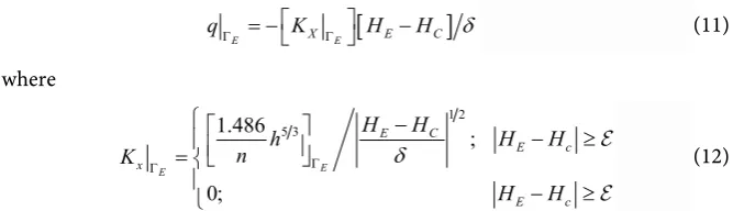
[image:4.595.206.540.487.583.2]di-rectly applied to a two-dimensional diffusion model with the selected (mX, my) relations incorporated. The two dimensional finite difference grid is shown in Figure 1.
4. Numerical Model Formulation (Grid Element)
For uniform grid elements, the integrated finite difference version of the nodal domain integration (NDI) method [1] is used. For grid elements, the NDI nodal equation is based on the usual nodal system shown in Figure 1. Flow rates (q = Qx/width) across the boundary Г are estimated by assuming a linear trial
func-tion between nodal points.
For a square grid of width δ, Equation (6) can be reduced to
[
]
E X E E C
qΓ = −K Γ H −H δ
(11)
where
53 1 2
1.486 ;
0;
E E
E C
E c
x
E c
H H
h H H
n K
H H
δ
Γ Γ
−
= − ≥
− ≥
(12)
In Equation (12), h (depth of water) and n (the Manning’s coefficient) are both the average of their respective values at C and E, i.e. h=
(
hC+hE)
2 and(
nC E)
2n= +n . Additionally, the denominator of KX is checked such that
X
K is set to zero if HE−HC is less than a tolerance ε such as 10−3 ft. The
net volume of water in each grid element, along the x direction, between time-step i and i + 1 is
E w
i
C r r
q q q
∆ = +
DOI: 10.4236/jwarp.2018.1012069 1179 Journal of Water Resource and Protection
Figure 1. Two dimensional finite difference analog.
2
i i
C C
H q t δ
∆ = ∆ ∗ ∆
for timestep i and i + 1 with ∆t interval. Then the model advances in time by
an explicit approach
1
i i i
C C C
H+ = ∆H +H (13)
where the assumed input flood flows are added to the specified input nodes at each timestep. After each timestep, the hydraulic conductivity parameters of Equation (12) are reevaluated, and the solution of Equation (13) reinitiated.
5. Equivalent DHM PDE Formulation
The mathematical statement for the DHM computational procedure, in finite
difference form, as used in the DHM computer program ([1] and
http://www.diffusionhydrodynamicmodel.com) was implemented using com-puter program EXCEL which was, in turn, applied to several test problem situa-tions including the Example problem presented below. The alternate PDE (or, equivalent PDE) that mathematically describes the one-dimensional (“1D”) formulation of the DHM is obtained by examining the limit as the spatial incre-ments and computational time step size used in the finite difference model both approach zero in value. Upon taking the limits, the equivalent (or alternate) PDE statement is
1 2 5
3 h h
h
X X α t
∂ ∂ + =∂
∂ ∂ ∂ (14)
where α represents the sum of relevant parameters including the gradient of the flow channel.
DOI: 10.4236/jwarp.2018.1012069 1180 Journal of Water Resource and Protection
It is noted that with a similar analysis, other computational models of PDE can be evaluated, and possible equivalent PDE statements derived, that describe what the computational model is actually delivering. The differences between the target PDE and the equivalent PDE provides another assessment of compu-tational modeling error to be considered along with the other typical assessment tools contained in the modelers toolkit.
6. EXCEL Analog of the DHM Alternate PDE
Using the computational statement for the DHM, the modelling grid can be re-duced in size, resulting, as mesh size approaches zero, in the alternate limiting numerical statement.
In order to investigate the alternate PDE form discussed above, the computer spreadsheet program, EXCEL, was used to compute a one-dimensional transient flow problem. A two-dimensional form can similarly be developed. The flow domain was established by the columns of the spreadsheet, with each column representing a single cell in the flow domain, defined by an elevation, width, and length. The time domain was established by the rows of the spreadsheet, with each row representing a single point in time, defined by the user-defined time-step. The programming code, Visual Basic, was used to solve the one-dimensional flow problem.
Flow depth was calculated at each cell based on the cell center (node), and at each timestep, by the following equation:
(
)
(
)
(
(
)
(
)
)
2NewDepth node
depth node volumeFlow node volumeFlow node 1 dimension
= + − −
where depth(node) = the flow depth of the cell at the previous timestep, new Depth(node) = the flow depth of the cell at the current timestep, volume Flow(node) = the flow volume between the cell and its adjacent cell to the east, volume Flow(node-1) = the flow volume between the cell and its adjacent cell to the west, and dimension = width (which is also equivalent to length of the cell).
To calculate the flow volume between cells, the following equation was used:
(
)
(
)
volumeFlow node =flowRate node timestep∗
where the flowRate(node) was defined as:
(
) (
)
(
)
(
5 3)
(
(
)
1 2)
flowRate node 1.486 ManningN dimension
avgDepth node wsSlope node
= ∗
∗ ∗
where ManningN = Manning’s coefficient, avgDepth = the average depth of the cell and its adjacent cell, and wsSlope(node) = the slope of the water surface ele-vation between adjacent cells.
7. Example Problem
DOI: 10.4236/jwarp.2018.1012069 1181 Journal of Water Resource and Protection one-dimensional effectively flat domain (0.001 ft in 4 ft) is subjected to a nearly sudden rise in water depth at x = 0 at model time t = 0. The boundary condition in the EXCEL formulation is implemented by increasing the flow depth at x = 0 over a small time interval until the target boundary condition value is achieved. A time step of 0.05 seconds, Manning’s N value of 0.03 and a slope of 0.001 were used in the analysis.
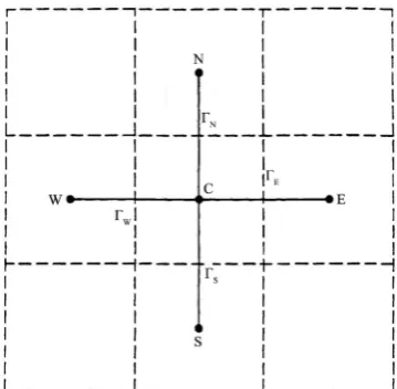
The resulting computational approximation results of the alternate PDE is shown in the solid lines in Figure 2. “EXCEL #1” illustrates the depth boundary condition vs. time in the most upstream computational element #1. “EXCEL #2” illustrates the resulting depth vs. time in the next downstream computational element #2; each succeeding computational element to #6 is similarly illustrated, showing the progression of the flow wave downstream.
To examine the equivalence of the alternate PDE to the DHM, a DHM model of the problem situation was developed and its computational results compared to the results of Figure 2. DHM model results for depths in DHM grid elements #1 to #6 are shown as dashed lines in Figure 2. Construction of the DHM grid-ding was a straightforward chain of 4 ft
×
4 ft grid elements, each with a rough-ness coefficient of 0.03. Slope was equivalent to 0.001 ft drop per 4-ft grid ele-ment. Grid element #1, the most upstream, had an arbitrary elevation of 100.000 ft. Grid element #2 next downstream, had an elevation of 99.999 ft, and so on down to grid element #20 which formed the outlet of the model. The outlet boundary condition was critical depth.The only inflow boundary condition available for the DHM floodplain is a flow hydrograph. The inflow boundary condition for the EXCEL model was an implied flow hydrograph such that depth in computational element #1 ramped up from zero at time zero to 1 ft at 1 second, then remained constant at 1 ft for the duration of the computation at 3 seconds. The problem then for the DHM model was to input a flow hydrograph that resulted in the depth vs. time rela-tionship in EXCEL computational element #1.
The inflow rate for the first 0.05 EXCEL time step was 16 cubic feet per second. While the resulting DHM depth profile approximated the EXCEL depth profile, cutting the DHM inflow at 1 second resulted in an overshoot and a depth equi-librium at 1.2 ft. Using this behavior as a baseline, the DHM inflow hydrograph was iteratively adjusted such that there was a very close match between profiles in element #1. Eleven trials were run. The final inflow hydrograph is provided in Table 1.
The comparison of flow profiles in Figure 2 illustrates the reliability of the solution from the proposed methodology.
8. Conclusions
DOI: 10.4236/jwarp.2018.1012069 1182 Journal of Water Resource and Protection
Figure 2. Comparison of transient flow depth profiles between the DHM and simplified model.
Table 1. Inflow hydrograph at Node # 1.
Time (hours) Flow (cfs)
0.0 2.78E−5 4.17E−5 5.56E−5 8.33E−5 1.11E−4 1.67E−4 2.08E−4 2.64E−4 2.78E−4 3.19E−4 4.17E−4 5.69E−4 6.25E−4 7.50E−4
16.000 16.160 16.320 16.640 17.600 18.880 24.000 35.000 50.000 50.000 40.000 21.357 25.065 24.529 22.896
[image:8.595.210.539.372.561.2]DOI: 10.4236/jwarp.2018.1012069 1183 Journal of Water Resource and Protection BVP. Once determined, the Alternate DHM is used to demonstrate the equiva-lence to the CEM formulation published for the DHM and in use since the early 1970’s. This Alternate DHM formulation provides significant advantages in the assessment of the performance and accuracy of DHM modeling estimates and predictions.
Resolution of the DHM computational model into its Alternate form, as ac-complished in the current paper, can be done for other computational models. It is recommended that such investigation be accomplished with other computa-tional models and the Alternate model formulation used for assessment of the modeling performance
Acknowledgements
A substantial amount of the material presented in the subject paper was au-thored by the paper’s first author in the original USGS Report, and the relevant portions are presented only for the reader’s convenience as modified for this pa-per. The authors wish to acknowledge the USGS and thank that agency for their permission to use this material as summarized in the current paper. The original full report and appendices are available at the subject USGS web site [1].
Conflicts of Interest
The authors declare no conflicts of interest regarding the publication of this pa-per.
References
[1] Hromadka, T.V. and Yen, C.-C. (1987) A Diffusion Hydrodynamic Model, U.S. Geological Survey. Water-Resources Investigations Report, USGS Publications Warehouse, 87-4137. http://pubs.er.usgs.gov/publication/wri874137
[2] Rao, P., Hromadka II, T.V., Huxley, C., Souders, D., Jordan, N., Yen, C.C., Bristow, E., Biering, C., Horton, S. and Espinosa, B. (2017) Assessment of Computer Model-ing Accuracy in Floodplain Hydraulics.International Journal of Modelling and Si-mulation, 37, 88-95. https://doi.org/10.1080/02286203.2016.1261218
[3] Hromadka II, T.V., Berenbrokc, C.E., Freckleton, J.R. and Guymon, G.L. (1985) A Two-Dimensional Diffusion Dam-Break Model. Advances in Water Resources, 8, 7-14. https://doi.org/10.1016/0309-1708(85)90074-0
[4] Hromadka, T., Walker, T., Yen, C. and DeVries, J. (1989) Application of the USGS Diffusion Hydrodynamic Model for Urban Floodplain Analysis. JAWRA Journal of the American Water Resources Association, 25, 1063-1071.
https://doi.org/10.1111/j.1752-1688.1989.tb05422.x
[5] Hromadka, T.V. and Yen, C.C. (1993) A Diffusion Hydrodynamic Model (DHM). Advances in Water Resources, 9, 118-170.
https://doi.org/10.1016/0309-1708(86)90031-X
[6] Hromadka, T.V., Yen, C.C. and Bajak, P.A. (1992) Application of the USGS Diffu-sion Hydrodynamic Model (DHM) in Evaluation of Estuary Flow Circulation. Ad-vances in Engineering Software, 14, 291-301.
DOI: 10.4236/jwarp.2018.1012069 1184 Journal of Water Resource and Protection [7] Hromadka II, T.V., Walker, T.R. and Yen, C.C. (1988) Using the Diffusion Hydro-dynamic Model (DHM) to Evaluate Flood Plain Environmental Impacts. Environ-mental Software, 3, 4-11. https://doi.org/10.1016/0266-9838(88)90003-2
[8] O’Brien, J.S., Julien, P.Y. and Fullerton, W.T. (1993) Two-Dimensional Water Flood and Mudflow Simulation. Journal of Hydraulic Engineering, ASCE, 119, 244-261.
https://doi.org/10.1061/(ASCE)0733-9429(1993)119:2(244)
[9] Singh, V.P. (1996) Kinematic Wave Modeling in Water Resources: Surface-Water Hydrology. Wiley, New York.
[10] Neil, H.M., Bates, P.D., Horritt, M.S. and Wilson, M.D. (2007) Simple Spatial-ly-Distributed Models for Predicting Flood Inundation: A Review. Geomorphology, 90, 208-225. https://doi.org/10.1016/j.geomorph.2006.10.021