Methods in spatially explicit capture recapture

(1)

Ben C. Stevenson

A Thesis Submitted for the Degree of PhD

at the

University of St Andrews

2016

Full metadata for this thesis is available in

St Andrews Research Repository

at:

http://research-repository.st-andrews.ac.uk/

Please use this identifier to cite or link to this thesis:

http://hdl.handle.net/10023/18233

This item is protected by original copyright

This item is licensed under a

Creative Commons License

(2)

CAPTURE-RECAPTURE

Ben C. Stevenson

A thesis submitted for the degree of

Doctor of Philosophy

at the University of St Andrews

(3)

(4)

Candidate’s declaration

I, Ben C. Stevenson, hereby certify that this thesis, which is approximately 53 000 words

in length, has been written by me, and that it is the record of work carried out by me,

or principally by myself in collaboration with others as acknowledged, and that it has not

been submitted in any previous application for a higher degree.

I was admitted as a research student in June 2012 and as a candidate for the degree of

PhD also in June 2012; the higher study for which this is a record was carried out in the

University of St Andrews between 2012 and 2016.

Date: 23/03/2016 Signature of candidate:

Supervisor’s declaration

I hereby certify that the candidate has fulfilled the conditions of the Resolution and

Reg-ulations appropriate for the degree of PhD in the University of St Andrews and that the

candidate is qualified to submit this thesis in application for that degree.

Date: 23/03/2016 Signature of supervisor:

Permission for publication

In submitting this thesis to the University of St Andrews I understand that I am giving

permission for it to be made available for use in accordance with the regulations of the

Uni-versity Library for the time being in force, subject to any copyright vested in the work not

being affected thereby. I also understand that the title and the abstract will be published,

and that a copy of the work may be made and supplied to any bona fide library or research

worker, that my thesis will be electronically accessible for personal or research use unless

exempt by award of an embargo as requested below, and that the library has the right to

migrate my thesis into new electronic forms as required to ensure continued access to the

thesis. I have obtained any third-party copyright permissions that may be required in order

to allow such access and migration, or have requested the appropriate embargo below.

The following is an agreed request by candidate and supervisor regarding the publication

(5)

Printed copy

Embargo on all of print copy for a period of two years on the following grounds:

• Publication would preclude future publication.

Electronic copy

Embargo on all of print copy for a period of two years on the following grounds:

• Publication would preclude future publication.

Supporting statement for electronic embargo request

The ability to publish work found within this thesis may be compromised if it is not

em-bargoed.

Date: 23/03/2016

(6)

(7)

(8)

Acknowledgements

I am grateful to both the Centre for Research into Ecological and Environmental Modelling

(CREEM) and the National Centre for Statistical Ecology (NCSE) for studentships that

provided funding for my studies. The NCSE studentship was available through a joint grant

from the Engineering and Physical Sciences Research Council and the Natural Environment

Research Council (#EP/1000917/1). Additional thanks to Auckland Grammar School, New

Zealand, for further support through the F. W. W. Rhodes Memorial Scholarship.

I was fortunate to obtain funding from a variety of other sources that allowed me to

undertake various worldwide adventures, and these greatly enriched my PhD experience.

In particular, I acknowledge Hans Skaug for funding to attend the 2013 ADMB developers’

meeting in Reykjav´ık, The National Geographic Society for a grant (via principal

investiga-tor John Measey) that part-funded a research trip to Cape Town, the University of Auckland

for part-funding a collaborative research visit to New Zealand, Monique MacKenzie for

tak-ing me along to teach workshops in South Africa and Ghana, and The American Statistical

Association for partial funding to attend the 2015 Joint Statistical Meetings in Seattle.

Despite ecological statistics being an interdisciplinary subject area, my previous training

has been anything but. I thank those people who have put up with my general ignorance of

the biological sciences—in particular John Measey and Res Altwegg, whose collaboration

contributed strongly to the content found in Chapter 3. I am particularly obliged to John

for proofreading passages from this thesis.

I am hugely indebted to Rachel Fewster. First, for being a fantastic collaborator (of the

statistical kind); of all statisticians I have met she must be one of the finest at explaining

her (usually complex) statistical ideas in an intuitive, understandable way. Furthermore,

a research retreat she organised (and funded through a Royal Society of New Zealand

Marsden grant) in the Scottish highlands has surely been one of the most productive weeks

of research over the course of my studies. Much of the work found in Chapter 6 is due to

this collaboration. Second, she was hugely influential in my decision to come to St Andrews

to pursue studies towards a PhD in the first place. Despite never having properly met,

in 2011 I organised a meeting with her enquire about the University of St Andrews as

a possible candidate institution for further study. I left that meeting with the strongest

recommendation to apply, and an excellent suggestion for a potential supervisor. I was

blown away by the effort she had made into determining what I—a virtual stranger—was

like (not only as a researcher, but as a person in general) in order to determine what would

be the ‘best fit’ for me at St Andrews. The subsequent decision of where I was to pursue

(9)

weather—she told me I would thoroughly enjoy working at CREEM.

And right she was. CREEM has provided the perfect working environment for my PhD

studies: it has been intellectually stimulating and engaging place to study, and comprises

the friendliest group of people I have ever had the pleasure of working with. I cannot name

everyone personally, but I would like to acknowledge, in general, all who make it the place

that it is. Thanks for the imparting your knowledge and advice (from some of the best

minds in the field no less); thanks for the general chit-chat at coffee, the typically British

small talk about how terrible the weather is, has been, and ever will be; and, of course,

thanks for the cake.

I would like to specifically mention a few people who have had a particular influence

on me during my time in St Andrews. I extend my gratitude to the following people:

To Darren—former officemate—for his friendship; for his sense of humour, which made

Room 115 such an enjoyable place to work; and for his contributions to discussions that

(in particular) enhanced my understanding of SECR, C++, and the R package Rcpp. To

Richard—replacement officemate and wise beyond his years—for all his perceptive advice:

from which Linux distribution I should install (Xubuntu) and how powerful my laptop’s

processor should be (Intel Core i7), through to whether the rows in Table 3.2 should refer

to parameters or confidence interval methods (the latter) and what type of cake I should

bake at the weekend (upside-down mango). To Charlotte (and Watson) for the games, the

adventures, and for keeping my chin up and a smile on my face—especially at times when

there did not appear to be much to smile about. Finally, to Cassandra, whose love and

support indirectly contributed to much of the work behind this thesis.

I make particular note of David Borchers, my supervisor, who has been outstanding from

the very beginning. I had originally found it difficult to engage academics in distant lands

for discussion about potential PhD studies at their institutions, often receiving generic

replies about the application process and how difficult it might be to find appropriate

funding. After sending David an initial e-mail expressing my interest in a PhD position

at St Andrews, I awoke the next day to an enthusiastic, comprehensive reply (in excess of

1 500 words) detailing all the research areas in which he would be interested in providing

supervision, and a range of potential funding options. His level of commitment to me and

my work has never faltered. Time and again he has shown (possibly blind) faith in my

abilities—for example, offering me the lead role of a project on the acoustic monitoring of

frogs early on in my studies, and later sending me in his stead to present an invited talk at

a leading international conference. He has allowed me the freedom to direct my research in

(10)

a hat for guidance and advice—not only about my research, but also on both personal and

professional matters—despite his newfound professorial responsibilities. David has been

everything I could have hoped for in not only a PhD supervisor, but also a mentor and

guide to life in academia. These words do not do justice to the level of appreciation that I

wish to convey.

Finally, a special thanks to my family back in New Zealand—Ollie, Kate, Nana, and

particularly my parents, Helen and Craig. They have always been incredibly supportive

of both my continued academic pursuits and my decision to undertake them on nearly the

most distant landmass possible. Although our geographical separation may be vast, they

have always been sure to maintain closeness in other (non-Euclidean) metrics. Thank you

for always being an e-mail, a message, or a video call away, and for providing a constant

(11)

(12)

Abstract

Capture-recapture (CR) methods are a ubiquitous means of estimating

ani-mal abundance from wildlife surveys. They rely on the detection and subsequent

redetection of individuals over a number of sampling occasions. It is usually

necessary for individuals to be recognised upon redetection. Spatially explicit

capture-recapture (SECR) methods generalise those of CR by accounting for

the locations at which each detection occurs. This allows spatial heterogeneity

in detection probabilities to be accounted for: individuals with home-range

cen-tres near the detector array are more likely to be detected. They also permit

estimation of animal density in addition to abundance.

One particular advantage of SECR methods is that they can be used when

individuals are detected via the cues they produce—examples include birdsongs

detected by microphones and whale surfacings detected by human observers. In

such situations each cue may be detected by multiple detectors at different fixed

locations. Redetections are then spatial (rather than temporal) in nature, and

density can be estimated from a single survey occasion.

Existing methods, however, cannot generally be appropriately applied to the

resulting cue-detection data without making assumptions that rarely hold.

Ad-ditionally, they usually estimate cue density rather than animal density, which

does not usually have the same biological importance. This thesis extends SECR

methodology primarily for the appropriate estimation of animal density from

cue-based SECR surveys. These extensions include (i) incorporation of

aux-iliary survey data into SECR estimators, (ii) appropriate point and variance

estimators of animal density for a range of scenarios, and (iii) methods to

ac-count for both heterogeneity in detectability and cues that are directional in

nature.

Moreover, a general class of methods is presented for the estimation of

demo-graphic parameters from wildlife surveys on which individuals cannot be

(13)

(14)

1 Introduction 1

1.1 Estimating animal abundance and density . . . 1

1.2 Spatially explicit capture-recapture . . . 5

1.3 Statistical notation . . . 8

1.4 Estimation . . . 9

1.5 Thesis overview . . . 14

2 A unifying model for capture-recapture and distance sampling 19 2.1 Introduction . . . 19

2.2 Incorporation of auxiliary information . . . 21

2.3 Theadmbsecrpackage . . . 29

2.4 Applications . . . 45

2.5 Discussion . . . 48

3 Cue-based SECR methods 53 3.1 Introduction . . . 53

3.2 Methodology . . . 56

3.3 Implementation inadmbsecr . . . 59

3.4 Simulation studies . . . 59

3.5 Applications toA. lightfooti survey data . . . 62

4 First-cue SECR methods 81 4.1 Introduction . . . 81

4.4 Simulation study . . . 93

4.5 Application toS. aurocapilla survey data . . . 94

(15)

5 SECR methods for cue directionality and strength heterogeneity 107 5.1 Introduction . . . 107

5.4 Simulation studies . . . 127

6 Uncertain identification in surveys of wildlife populations 135 6.1 Introduction . . . 135

6.2 TC models . . . 145

6.3 Thenspp package . . . 155

6.4 Application to two-plane cetacean surveys . . . 159

7 Discussion 171 7.1 Integrated cue-rate estimation from SECR surveys . . . 172

7.2 Animal movement in cue-based SECR surveys . . . 177

7.3 Concluding remarks . . . 179

References 183

Acronyms 193

Names of species 197

Notation (Chapters 1–5) 199

(16)

(17)

(18)

Introduction

1.1 Estimating animal abundance and density

Animal abundance refers to the absolute number of individuals (usually of a particular

species) that inhabit a particular site of interest. Animal density is the quotient of the

abundance and the area of this site. Both variables are of great ecological importance:

ecology has practical applications in a variety of fields, and for many of these it is necessary

to estimate either abundance or density of animal species. Consider a conservation biologist

who wishes to track the population size of a newly endangered species, a wildlife

manage-ment consultant who is required to establish the efficacy of a recent pest eradication, and a

policymaker looking to reduce the daily bag limit for recreational fishers in order to preserve

the sustainability of a fishery. All require some method of gaining information about the

density or abundance of at least one animal species.

In almost all cases an attempt to count each and every individual within the entire

region of interest is infeasible. While these census methods are the only way of obtaining

errorless measurements of abundance and density, they are also time consuming, they can

be financially prohibitive, and are often practically or logistically impossible. In order to

alleviate these burdens one may (i) only sample a subset of the region of interest, and (ii)

forgo an exhaustive search, accepting that some individuals will be missed. While these

practices decrease fieldwork effort, they introduce uncertainty: one must account for both

the number of individuals outwith the searched area, and the number of individuals within

the searched area that were missed. Neither can be known with certainty.

Estimating the probability of detecting individuals is central to (ii), above. A wealth of

methods designed to estimate these detection probabilities (and therefore animal abundance

or density) can be found in the statistical ecology literature. Two common approaches exist:

(19)

0 2 4 6 8 10 0.0

0.2 0.4 0.6 0.8 1.0

Distance from transect

[image:19.612.91.518.97.263.2]

Probability of detection

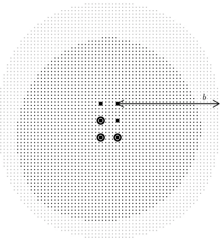
Figure 1.1 A histogram of simulated distances to animals detected by observers walking along a line transect. Truncation distance was set atw= 10. The detection function used to simulate these data, g(d), is overlain. The height of the histogram bars are scaled so that their collective area is equal toRw

0 g(x) dx, the area beneath the detection function.

distance sampling (DS) and capture-recapture (CR). These are outlined below, along with

mark-recapture distance sampling (MRDS), an approach that generalises DS via ideas from

the CR literature.

1.1.1 Distance sampling

See Buckland et al. (2001) and Buckland et al. (2004) for general overviews of DS

method-ology. A DS survey is carried out by observers who either travel along line transects or

are stationed at points. When an observer detects an individual (or group, if they occur in

groups) they record its distance from either the line or the point. Any observations beyond

some truncation distance w are ignored. If transects are placed at random, then the

un-derlying distribution of all distances to individuals (detected or otherwise) within distance

w is uniform on the interval [0, w] for lines, or has probability densityf(d)∝d, d∈[0, w],

for points. However, as animals closer to the observer are more easily detected, there are

a disproportionate number of detected individuals at shorter distances. The distribution

of the observed distances allows estimation of a detection function—a mathematical

func-tion returning the probability of detecting an individual a given distance from the observer

(Figure 1.1).

Obtaining an estimate of animal density involves the estimation of the proportionp, of

all individuals within the truncation distance that were detected. As an example, for

(20)

and the hypothetical detection function that arises from perfect detection (the dashed line in

Figure 1.1), respectively. Let the total number of detections be n. An abundance estimate

for the area searched (or sampled, i.e., the area within truncation distance w of the line

or point) is n/p_b. Calculation of this area is straightforward: for a line transect of length l

the sampled area is 2lw, and for a point the sampled area is πw2_{. As density is obtained}

by dividing abundance by the area searched, a density estimate Db is given byn/(2l b

pw) for

lines and n/(πpw_b 2) for points.

The denominator in both cases is the estimated effective sampling area (ESA), here

given by _ba. This is an estimate of the true ESA, a, and is the estiamted area of a region

within which the expected number of individuals isn. For example, if a line transect survey

is carried where the total area sampled is 100 m2 but the detection function is such that

only half of all individuals within distance w were detected (i.e.,p= 0.5), then the ESA is

0.5×100 = 50 m2. Density estimates can equivalently be seen as the quotient of the number

of detections made and the estimated ESA; that is, Db =n/_ba. Also note that an estimate of

animal abundance can be directly obtained by taking the product of the density estimate

and the area of the site of interest.

1.1.2 Capture-recapture

CR methods (also known as ‘mark-recapture’ and ‘capture-mark-recapture’) have a long

history in the field of abundance estimation, with the first such applications dating back

to the estimation of the populations of seventeenth-century London (Graunt, 1662) and

eighteenth-century France (Laplace, 1786). Here, only the estimation of closed

popula-tions (i.e., those without births, deaths, immigration, or emigration) is considered. Seber

(1982) and Borchers, Buckland, and Zucchini (2002) provide overviews of various such CR

approaches.

The underlying idea is straightforward: traps are laid out at fixed locations and these

are used to physically capture animals. Individuals are captured on discrete sampling

oc-casions in such a way that it is known with certainty when the same individual is captured

again. This usually involves marking animals (e.g., by using a tag), but can alternatively

rely on later recognition based on natural features (e.g., tigers’ stripe patterns). The

ob-served data arecapture histories—one for each detected individual—denoting the sampling

occasions on which the animals were detected. These data allow direct estimation of capture

probabilities.

In general, animals need not be physically detained by traps, but can instead be detected

(21)

‘detector’ and ‘detections’ are henceforth used instead of traditional terms related to ‘traps’

and ‘captures’1.

As a simple example, consider a CR survey with just two discrete sampling occasions.

Let the number of individuals detected on occasion i be ni, the number of individuals

captured on both occasions i and j be nij, and total abundance (the main parameter of

interest) beN. Assume that capture events are independent across occasions and between

individuals, and that the probability of capture p is the same for all individuals. A simple

estimate for p is given by p_b= n12/n1; that is, the proportion of individuals marked on

the first occasion that were detected again on the second occasion. An estimate for total

population size can be calculated by scalingn2 to account for undetected individuals; that

is, Nb = n₂/p_b. This is the Lincoln-Petersen method of population abundance estimation;

see Seber (1982) for further details. Alternative estimators are available for surveys with

more than two capture occasions.

The assumption of a constant detection probability,p, across all individuals and over all

capture occasions is seldom reasonable in practice. Otis, Burnham, White, and Anderson

(1978) summarised various extensions to constant-probability models to allow for changes

in detection probabilities (i) across time (denoted modelMt), (ii) across individuals (model

Mh), and (iii) following an individual’s first capture (e.g., due to trap-shy or trap-happy

behaviour; modelMb). Combinations of the above can also be incorporated into the same

model (e.g., modelMtbh to account for all three).

Unlike DS, CR methods do not have a spatial component. A consequence of this is that

it is impossible to directly estimate density from the CR data alone—the sampled area is

not known and model parameter estimates do not give rise to an estimate of the ESA. An

estimate of abundance, Nb, can be problematic to interpret without an associated area: if

the spatial range of the traps or detectors is small in comparison to the spatial range of the

locations at which members of the population of interest live, then it is generally impossible

to determine total population size—only those individuals that roam near the detectors are

available for detection, and it is not possible to estimate the proportion of the population

that this constitutes.

1.1.3 Mark-recapture distance sampling

A necessary assumption for many DS models is that detection is certain for animals situated

directly on the transect (for line transect surveys) or at the observer location (for point

transect surveys). MRDS methods (Borchers, Zucchini, & Fewster, 1998; Manly, McDonald,

1

(22)

& Garner, 1996) extend DS by including multiple, independent observers—each of whom

can be considered a separate detection ‘occasion’. This therefore uses ideas from both DS

and CR: the CR component allows for estimation of the probability of detections at distance

zero (i.e., animals either on the transect or at the point), while the DS component allows for

the estimation of a detection function and a model for the distribution of observed distances.

The observers typically travel along the same transect (for line-transect surveys) or are

situated on the same platform (for point-transect surveys; although in theory this need not

necessarily be the case), and in both cases it is possible for the same animal to be detected

by more than one observer. Detected individuals must be recognisable across observers in

order to construct a capture history for each. A further important component is that the

locations of detected animals on MRDS surveys are usually directly observed without error.

1.2 Spatially explicit capture-recapture

1.2.1 Overview

While model Mh (Otis et al., 1978) accounts for heterogeneity in detectability across

indi-viduals, CR methods do not directly model the obvious spatial component of these

prob-abilities: individuals are more likely to be captured if they live and roam near the

de-tectors. The relatively recent advent of methods that do incorporate spatial effects into

detection probabilities fall into a class of model known asspatially explicit capture-recapture

(SECR), although the term ‘spatial capture-recapture’ is also used. The first

implementa-tion of SECR models (Efford, 2004) relied on inverse predicimplementa-tion for parameter estimaimplementa-tion.

Maximum-likelihood (ML; Borchers & Efford, 2008) and Bayesian (Royle & Young, 2008)

approaches followed shortly thereafter.

Regardless of the estimation method, SECR marries the spatial component of DS and

the temporal nature of CR. A notable difference between SECR and CR is that CR models

ignore the locations at which detections of individuals are made, while this information is

retained in SECR. Capture histories for SECR therefore do not only include temporal

detec-tion informadetec-tion (i.e., the occasions on which an individual was detected), but also spatial

detection information (i.e., where these detections occurred). This allows for the estimation

of two additional model features: (i) the distribution of activity centres (sometimes called

the ‘home range centres’) of the individuals, which can often be thought of as the animals’

homes (e.g., their nests or burrows); and (ii) parameters of a detection function, returning

the probability of detection given an activity centre distance dfrom the detector. Together

(23)

● ● ● ● ● ● ● ● ● ●

● ● ● ● ● ● ● ●

● ● ● ● ● ● ● ● ●

● ● ● ● ● ● ● ●

● ● ● ● ● ● ● ● ●

● ● ● ● ● ● ● ● ● ●

● ● ● ● ● ● ● ● ●

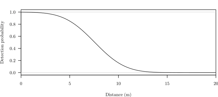
[image:23.612.202.508.120.343.2]

100 m

Figure 1.2 A depiction of three hypothetical capture histories from an SECR survey carried out using a grid of100 detectors. Detector locations are plotted. An open plotting character represents a location of a detector that detected one of the three individuals, where each plotting character type represents a different individual.

for individuals with activity centres at any point in the survey region—thus quantifying

interanimal heterogeneity in this regard. This also allows for the estimation of the ESA

from the survey data alone, which is not otherwise possible using CR methods.

See Figure 1.2 for an example. From these data one can infer the approximate location

of each individual’s activity centre, as well as information about the detection function. In

this case, it seems unlikely that a detector will detect an individual at a distance of more

than 100 m from its activity centre. This, in turn, provides information about the sampled

area (and thus animal density), which is usually unavailable in traditional CR analyses.

1.2.2 Spatial redetection

Initial implementations of SECR methodology relied on detection across discrete sampling

occasions, as typically found in traditional CR surveys. Efford, Dawson, and Borchers

(2009) made a further generalisation by noting that if redetections occur over a spatial

dimension within the same sampling occasion (i.e., redetections of the same individual occur

(24)

and density parameters are estimable from only that sampling occasion alone.

This often occurs by virtue of individuals producingcues—stimuli emitted by animals

that indicate their presence. Individuals may produce multiple cues, each of which may be

detectable. Examples include songs produced by songbirds and surfacings of whales. In

both cases, each cue may be simultaneously detected acoustically by multiple microphones

(for the former) or visually by multiple human observers at fixed locations (for the latter).

Conceptually, Figure 1.2 can be reconsidered with detectors as microphones, and open

plotting characters representing locations of microphones that detected a particular cue

produced by a particular individual.

Spatial redetection can also occur on surveys in which individuals do not emit cues that

are detected by multiple detectors—sometimes this is instead induced by the movement of

the animal itself. Common examples include camera-trap and hair-snag surveys; within

the same sampling occasion an individual may be detected by cameras or snags at quite

different locations. A further example that lies between the two above (cue and noncue)

situations is that of scat surveys: each individual produces multiple cues (scat), however

each is only ever once at a single location. The spatial range of detected scat produced by a

particular individual is again due to its movement, rather than the propagation of the cue

through space (cf. acoustic detection of animal vocalisations).

Surveys using spatial redetection methods hold a number of inherent advantages over

those that require the physical detection of individuals over multiple occasions: (i) having

only a single sampling occasion often results in cheaper and quicker surveys, particularly

if the survey location is remote; (ii) spatial redetection methods tend to be passive in

that individuals are not physically captured—passive detection is often less intrusive and

safer (for the surveyors as well as the animals) than methods that require physical capture

and tagging; (iii) these make SECR analyses possible for a larger number of species—for

example, acoustic detection is useful for species that are visually cryptic and difficult to

trap, but produce audible calls or can be detected by well-positioned camera traps.

There are certain similarities between the data collected for SECR with spatial

rede-tection and those collected on MRDS surveys: in both cases, each animal can be detected

by multiple detectors (perhaps human observers) that are situated at (potentially) different

points in the survey region. An important distinction here is that the locations of detected

individuals are assumed to be observed without error for MRDS, while this is not typically

the case for SECR surveys. For the latter, only the locations of thedetectors are known.

All methods discussed in this thesis refer to situations with cue-induced spatial

(25)

Table 1.1 Examples of capture histories of the same hypothetical data with various definitions for the unit of detection. Each of the detector columns indicates which units were detected by the corresponding detector. A1indicates that the detector detected the unit, a0indicates that it did not. Tables (a) and (c) are cue-based capture histories, and so cue identification numbers are included. All tables include individual identification numbers.

(a) Cues as units of detection.

Detector

Cue ID A B C D

1 1 1 0 1 0

2 1 0 0 1 0

3 1 1 1 0 0

4 2 0 0 0 1

5 3 0 1 1 0

6 3 0 0 0 1

(b) Individuals as units of detec-tion.

Detector

ID A B C D

1 1 1 1 0

2 0 0 0 1

3 0 1 1 1

(c) First cues as units of detec-tion.

Detector

Cue ID A B C D

1 1 1 0 1 0

4 2 0 0 0 1

5 3 0 1 1 0

1.2.3 Units of detection

For surveys on which individuals are detected from their cues, multiple cues from the same

individual may be detected. Prior to analysis, the unit of detection must be appropriately

defined. A natural choice is to select cues as the unit of detection, and so each detected

cue contributes a capture history for analysis (e.g., Table 1.1a), giving rise to cue-based

capture histories. Alternatively, individuals may be selected as the unit of detection, and so

each detectedindividual contributes a single capture history for analysis (e.g., Table 1.1b),

giving rise to individual-based capture histories. In this case, a detector is considered to

have detected an individual if the detector detected at least one of its cues. Finally, the first

detected cue from each individual may be used as the unit of detection (e.g., Table 1.1c),

giving rise to first-cue-based capture histories. Dawson and Efford (2009) were the first to

use this particular unit.

There are advantages and disadvantages associated with each of the three options—these

are discussed throughout this thesis. Note that capture histories with either individuals or

first cues as the unit of detection can only be created if individuals are recognisable from

their cues (i.e., it is known with certainty whether or not any two detected cues were

(26)

1.3 Statistical notation

Throughout Chapters 2–5, in order to prevent cumbersome notation, there is no explicit

notational distinction made between a random variable and a fixed value in the support

of its distribution—although any ambiguity will be resolved in writing (e.g., by stating

‘the random variable x’ or ‘the observed value x’). Furthermore, f(·) is used to denote a

probability density function (PDF; for a continuous random variable) or probability mass

function (PMF; for a discrete random variable), while F(·) is used to denote a cumulative

distribution function (CDF). Parameters corresponding to the distribution associated with

the probability density functions (PDFs), probability mass functions (PMFs), CDFs, and

other functions are typically separated from the arguments by a semicolon. Expectations

and variances of random variables are denoted by the functions E(·) and Var(·), respectively.

Again, to preserve clarity, PDFs, PMFs, and CDFs do not typically explicitly indicate

the corresponding random variable(s) to which they apply, as these should be clear from the

arguments the function takes. An exception is made when ambiguity threatens, in which

case a subscript following the function indicates the random variable it is associated with.

For example,f(x;θ) may be used generically to give the value of the PDF of the continuous random variablex(associated with a distribution characterised by the parameter vectorθ) at some fixed value x, whilefx(0;θ) is the evaluation of the same PDF at the value 0.

In general, bold lowercase font is used to denote a vector, while bold uppercase font is

used to denote a matrix. Plain font denotes a scalar.

Chapter 6 does not involve the development of SECR methodology. The above does

not apply, and notation specific to this work is described therein. A summary of almost

all notation used throughout is available in two lists of notation (one for Chapters 1–5 and

another for Chapter 6), found after the reference and acronym lists at the end of this thesis.

These lists are comprehensive and should be consulted regularly—acronyms and notation

are fully defined on first use, but not necessarily again.

1.4 Estimation

While the current surge in SECR methodological development is occurring under both the

classical and Bayesian paradigms, throughout this thesis estimation is solely under the

former (though this is not due to any ideological disposition held by the author).

This section formulates a basic likelihood, similar to that presented by Efford, Dawson,

and Borchers (2009), for spatial-redetection SECR methodology. Aside from Chapter 6,

(27)

modifications and additions to this likelihood. In particular, the development below does

not apply for methods in which first cues are the unit of detection.

1.4.1 SECR notation

In total, m detectors of fixed and known location detectn units of detection (either

indi-viduals, cues, or first cues; see Table 1.1) over the course of a survey of duration t. The

capture history for theith unit is given byωi, where ωij = 1 if it was detected by thejth

detector, and ωij = 0 otherwise. Capture histories for all detected units are contained in

the matrixΩ, theith row of which is given by ωi.

Let the survey region be denoted byA; this is the set of all habitable points at which

a detected unit may be located. The location of the ith detected unit within the survey

region is given by the Cartesian coordinatesxi= (xi1, xi2)∈ A, and locations of all detected individuals are held in the matrixX. At times, xis used generically to denote some point in the survey region that is not associated with any particular individual. Letdj(x) be the

Euclidean distance between the location x and the jth detector. At times, d is used as a scalar to indicate some distance (e.g., as an argument to a detection function).

In general, SECR methods allow for estimation of a density surface, providing

informa-tion not only about overall density, but also how it changes over the survey region. Here,

however, only estimation of an unchanging density acrossA is considered, and this

param-eter is given byD. The definition of the units of detection provide the measurement unit

of D: if individuals are detection units, thenD is the density of individuals, while if cues

are detection units, thenDis the density of cues (i.e., cues emitted per unit area per time

t). The vectorγ contains parameters of the detection function,g(·), and let θ= (D,γ).

1.4.2 The likelihood

Detection probabilities

The parametric function chosen to use as the detection function is achieved via a model

selection approach. Two common choices are thehalf-normal,

g(x;γ) =g0 exp ₋

x2

2σ2

, γ = (g0, σ), (1.1)

and thehazard-rate,

g(x;γ) =g0

1−exp

−x

σ

−z

(28)

detection functions.

The probability of thejth detector detecting a unit located atx is g(dj(x);γ), by the

definition of the detection function. Assuming independent detections across detectors, the

probability that a unit at xis detected by at least one detector is

p(x;γ) = 1−

m

Y

j=1

[1−g(dj(x);γ)], (1.3)

where the product provides the probability of the unit evading detection. The function

p(x;γ) is referred to as the detection probability surface (DPS). As detectors are more likely to detect closer units, this surface is typically at its highest at points in the survey

region close to the detectors, and approaches zero at locations further away.

Probability density of unit locations

Throughout methods in ecological statistics, it is often assumed that the locations of all

individuals within the survey region (regardless of whether or not they were detected) are

a realisation of a Poisson point process (e.g., Buckland, Oedekoven, & Borchers, 2016;

Cormack & Jupp, 1991). This implies that their locations are independent of one another.

Here such processes with homogeneous intensity Dare considered.

The below only holds if individuals are the unit of detection. When this is the case,

locations of detected individuals (and therefore units) are a realisation of a thinned Poisson

point process, where the thinning is through the DPS (Equation (1.3)). The marginal PDF

of the location of the ith detected individual is therefore

f(xi;γ) =

p(xi;γ)

R

Ap(x;γ) dx

, (1.4)

and so the location of a detected individual is most likely to be at a point in A close to

at least one detector, and unlikely to be at a point far from all detectors. Due to the

aforementioned independence,

f(X|n;γ) =

n

Y

i=1

f(xi;γ). (1.5)

The denominator of Equation (1.4) gives the ESA:

a(γ) = Z

A

(29)

As detected individuals’ locations are a realisation of a thinned Poisson point process,

the total number of units detected is a random variable that has a Poisson distribution.

Thus

n∼Poisson(µ),

where

µ= E(n) =D

Z

A

p(x;γ) dx,

and so

f(n;θ) = µ

n_e−µ

n! . (1.7)

If cues are the unit of detection the above is unlikely to hold: locations of cues emitted

by a particular individual are the same if it is stationary, and likely to be similar (thus

not independent) if it is not. It follows that the joint PDF of the locations of detected

units cannot be obtained via a product of the marginal densities, as per Equation (1.5).

Furthermore—given that the number of individuals is a Poisson random variable—the

dis-tribution of the number of detected cues is unclear, and so Equation (1.7) no longer holds.

Probability mass of capture histories

The details of this section hold regardless of how the unit of detection is defined. Given the

ith detected unit’s location, the PMF of its capture history is

f(ωi|xi;γ) =

Qm

j=1g(dj(xi);γ)ωij[1−g(dj(xi);γ)]1−ωij

p(xi;γ)

. (1.8)

The numerator is a product across all detectors, where a detector contributes the probability

of detection to the product if it detected the individual, or the probability of evasion if it

did not. A capture history can only be observed if at least one detector makes a detection

(i.e., observing ωi is conditional on Pm_j₌₁ωij > 0) thus this product must be divided by

Pr(Pm

j=1ωi >0)≡p(xi;γ) to account for the fact that a capture history of0m cannot be

(30)

Assuming independence between individuals gives the result

f(Ω|n,X;γ) =

n

Y

i=1

f(ωi|xi;γ). (1.9)

The likelihood function

The likelihood is the joint density of the observed data, as a function of the model

param-eters; that is,

L(θ;n,Ω) =f(n,Ω;θ)

=f(n;θ)f(Ω|n;γ). (1.10)

The first term in the above product is available from Equation (1.7). For the second, there

is obvious dependence between ΩandX: detectors are more likely to detect units they are close to, and less likely to detect those that are far away. Unit locations are unobserved,

however, and so are modelled as latent variables. They are therefore incorporated into the

PMF of Ωvia integration over the survey region:

f(Ω|n;γ) = Z

An

f(Ω,X|n;γ) dX

= Z

An

f(Ω|n,X;γ)f(X|n;γ) dX. (1.11)

In general this 2n-dimensional integral is intractable, and at best its approximation is

extremely computationally expensive. Assuming independence across units (both between

their capture histories, conditional on location, and between their locations) allows for

separability due to Equations (1.5) and (1.9), giving

f(Ω|n;γ) = Z

An

n

Y

i=1

[f(ωi|xi;γ)f(xi;γ)] dX

= Z

A

· · ·

Z

A

n

Y

i=1

[f(ωi|xi;γ)f(xi;γ)] dx1· · ·dxn

=

n

Y

i=1 Z

A

f(ωi|xi;γ)f(xi;γ) dxi. (1.12)

The terms in the above integrand are available from Equations (1.8) and (1.4), respectively.

Approximation of this product of n two-dimensional integrals is substantially more

(31)

numerator of the second term (Equation (1.4)) in the integrand cancel. Furthermore, the

numerator of the latter is a constant with respect to the integral and can be moved out of

the integrand.

Estimation of θ is via maximisation of the likelihood, and so

b

θ = arg max

θ

L(θ;n,Ω). (1.13)

1.5 Thesis overview

This thesis outlines a variety of methods aimed at improving animal abundance and density

estimation from SECR survey data. With the exception of Chapter 6, the following chapters

describe novel methods that involve generalisations and other modifications to the likelihood

presented above.

A reference list immediately follows Chapter 6. Throughout this thesis, the first time a

species is mentioned both common and binomial names are given; subsequently it is only

referred to by the latter. A species list providing both common and binomial names appears

after the reference list, and before the notation lists.

This section provides an overview of each chapter.

1.5.1 A unifying model for capture-recapture and distance sampling

With traditional SECR methodology information about an individual’s location comes

solely from the locations at which it is detected (see Figure 1.2). Surveys that collect

data appropriate for analysis with SECR methods—particularly those that involve spatial

redetection—are often capable of obtaining auxiliary data that may provide additional

in-formative spatial information. For example, human observers acting as either visual or

acoustic detectors may not only record whether or not they detected a particular

individ-ual, but they may also estimate a bearing or distance to the detected animal. Furthermore,

acoustic detectors (such as microphones) may automatically measure strengths and

pre-cise times of arrival of detected signals. Detectors closer to an individual should expect to

receive shorter estimated distances, and louder and sooner received signals.

In Chapter 2 methods for incorporating such auxiliary information into animal density

estimators are described. It is shown that using such information can substantially improve

estimator precision and also reduce bias. CR and DS are both special cases of this new

model class, putting them at opposite ends of a spectrum of methods that vary in terms of

(32)

Furthermore, it is noted that existing software does not generally allow for incorporation

of these auxiliary data into SECR analyses. A new package for the R software environment

for statistical computing and graphics (R Core Team, 2015) known as admbsecr is

intro-duced. It is specifically designed for the analysis of data from SECR surveys on which

auxiliary data has been collected. Chapter 2 therefore also describes this software package,

and provides examples of its use. Indeed, many methods introduced in this thesis are

im-plemented in the admbsecr package, and so its use is also shown throughout many of the

following chapters.

1.5.2 Cue-based SECR methods

Section 1.4.2 provides comprehensive details of a likelihood for SECR methods when

indi-viduals are the units of detection. There are a number of issues that must be addressed

for its use with cue-based capture histories. For example, (i) due to dependence between

locations of cues emitted by the same individual, deriving the PMF of the number of

de-tected units (Equation (1.7)), and the joint PDF of unit locations (Equation (1.5)) is not

straightforward—these components remain unspecified for cue-based SECR methods; (ii)

the simplification of an otherwise intractable likelihood function (Equation (1.12)) is only

possible when the independence between locations holds; and (iii) the parameter D is cue

density, but animal density is usually of interest.

The only published method for the analysis of cue detection data using SECR (Efford,

Dawson, & Borchers, 2009) has involved a likelihood with the same features as that shown

above. The approach is described implicitly assuming that no more than a single cue from

each individual is detected; the assumption of independence between detected cues is

there-fore reasonable, andDcorresponds to animal density. However, surveys are likely to record

detections of multiple cues from each individual, and it is not clear how the method can be

put into practice when this is the case. These shortcomings were not explicitly stated by

Ef-ford, Dawson, and Borchers (2009), and as a result a subsequent application of their method

to acoustic detection data of the common minke whale Balaenoptera acutorostrata

(Mar-ques et al., 2012; Martin et al., 2013) involves the analysis of multiple cues per individual,

despite the concerns addressed above.

In Chapter 3 the consequences of violating the assumption of independence between cue

locations is explored, and methods for obtaining appropriate point and variance estimates

of animal density from cue-based capture histories are described. These are applied to data

(33)

1.5.3 First-cue SECR methods

The method of Efford, Dawson, and Borchers (2009) has also been applied to acoustic

detection data of the ovenbirdSeiurus aurocapilla (Dawson & Efford, 2009). In an attempt

to meet the assumptions of the method only the first detected call from each detected

individual was considered eligible for analysis. This can only be achieved if individuals are

identifiable from their cues. However, this results in the estimation of acue-based detection

function; that is,g(d;γ) andp(x;γ) return the probabilities (at a single detector, and across an array of detectors, respectively) that a particularcue is detected. This is not appropriate

when attempting to estimate animal density, as the probability of a single cue being detected

is not equivalent to the probability of a particular animal being detected. Cues do not have

a temporal component of detection as they occur at a (virtually) discrete point in time;

however, individuals do have such a temporal component: the longer a survey, the more

times an individual is likely to emit a cue—thus it is more detectable, and its detection

probability is necessarily higher.

In Chapter 4 it is shown that estimating animal density using the method of Efford,

Dawson, and Borchers (2009) by only including the first detected cue in the set of capture

histories to analyse (e.g., Table 1.1c, and as per Dawson & Efford, 2009) is not appropriate,

and that this practice can potentially result in substantially biased inference. Furthermore,

a likelihood is derived, maximisation of which results in an animal density estimator with

negligible bias that is shown to perform at least as well in all situations for first-cue capture

histories (as per Dawson & Efford, 2009) as that proposed by Efford, Dawson, and Borchers

(2009).

1.5.4 SECR methods for cue directionality and strength heterogeneity

The likelihood presented in Section 1.4.2 assumes that the detection probability of a cue

at a particular detector only depends on the distance between their respective locations.

Additionally, detections across the detectors are assumed to be independent, conditional

on the cue’s location (see Equation (1.8)). These features imply (i) that cues are equally

detectable in all directions, and (ii) that all cues are equally detectable. This is consistent

throughout the methods introduced in Chapters 3 and 4. These assumptions are not always

realistic, particularly for acoustic surveys. Calls from some species are very directional, and

are far more detectable in the direction they are emitted. For others, there may be marked

heterogeneity in the strength a cue is emitted, so that some cues are more detectable than

others.

(34)

either cue directionality (CD) or cue strength heterogeneity (CSH). They do not require the

direction or cue strength to be observed—instead, they are able to estimate these features

of the call. It is shown that estimators from these methods outperform those that ignore

CD and CSH.

1.5.5 Uncertain identification in surveys of wildlife populations

Analysis of data collected from wildlife surveys often requires each detected animal to be

identified and subsequently recognised at each redetection. This holds for SECR surveys,

and indeed the methods presented in the aforementioned chapters all rely on the ability to

ascertain which cues detected across an array were emitted by the same source.

Traditionally, CR surveys achieve identification by physically capturing and tagging

individuals. With recent advancements in wildlife monitoring technology there is no longer

the need to physically detain individuals—monitoring using cameras, microphones, and

the like are gradually becoming commonplace. These allow the collection of more data

than ever before despite a greatly reduced fieldwork burden. Identification approaches

involve recognising unique features of individuals (such as scars, natural patterns, or acoustic

signatures), or from genetic identification (from samples of hair or scat). However, these

methods do not come with the same identification certainty as a securely fastened tag:

similar physical or acoustic features (for visual or acoustic identification) and allele dropout

(for genetic identification) introduce uncertainty into the identification of individual animals.

In Chapter 6 a method is developed for the estimation of whale density from an aerial

survey on which planes fitted with high-definition cameras monitor a transect. Surfacing

whales can be detected from the collected images. Density is not estimable if just a single

plane is deployed, as the proportion of whales that were detected (and therefore those that

remained undetected) is not known. There is potential for this proportion to be estimated if

multiple planes are used: if individuals can be recognised across images collected by different

planes the data collected can be analysed using straightforward CR methods, where each

plane can be thought of as a capture occasion.

However, individuals cannot be recognised, and the method that is presented accounts

for this identification uncertainty. It is one of the first members of a class recently coined

as trace-contrast (TC) models. There is potential for the development of further related

models of this class to provide a way of accounting for uncertain identification in a range

(35)

(36)

A unifying model for

capture-recapture and distance

sampling

2.1 Introduction

As presented in Sections 1.1.1 and 1.1.2, one fundamental difference between traditional DS

and CR methods is that DS incorporates the locations of detected animals (as distances

from observers’ locations), while CR does not. SECR methods sit in between: locations

(e.g., of animals’ activity centres, if traps are used as detectors) are not directly observed,

but are nevertheless modelled as latent variables. Noisy information about the location

associated with each detection unit is therefore held in its capture history—an individual

is most likely to be close to the locations of the detectors that made a detection.

Remote detectors are often capable of collecting additional noisy information about

locations associated with the detection units. Let Y contain all such information collected from all detections and ψ be a vector containing parameters required to model these data. Four types of such information are specifically dealt with in this chapter; these are (i)

estimated bearings to detected animals, (ii) estimated distances to detected animals, (iii)

received acoustic signal strengths and (iv) received acoustic signal times of arrival (TOAs).

Intuitively, the more information incorporated into statistical models the higher the

precision of the resulting estimators. Reduced uncertainty about detection unit locations

provides cleaner information about the distances between these locations and the detectors;

this, in turn, allows the detection function parameters, γ, to be estimated with more pre-cision, and one would expect the reduced uncertainty to propagate through to the density

(37)

estimator.

A recent result also provides theoretical justification. Fewster and Jupp (2013) showed

that incorporation of additional data sources into parameter estimators will result in

con-fidence intervals (CIs) that are asymptotically narrower, despite the requirement for

addi-tional nuisance parameters. Thus, estimation via maximisation of a likelihood incorporating

these auxiliary data,

(D,b γ_b,ψb) = arg max

D,γ,ψ

L(D,γ,ψ;n,Ω,Y), (2.1)

is preferable to that shown in Equation (1.13), as long as Y provides some information about the parameter of interest,D.

In this chapter, the likelihood shown above, L(D,γ,ψ;n,Ω,Y), is derived, allowing estimation that incorporates general auxiliary information types (Section 2.2). For this

likelihood individuals are defined as detection units, and soDb is the estimated animal

den-sity. It is shown that this likelihood is equivalent to those used for density estimation with

MRDS and DS methods in the special case whenY provides perfect, noiseless information about detected animals’ locations. Moreover, it is equivalent to those used for abundance

estimation with standard CR methods when there is no spatial effect on detection

proba-bilities. This thus unifies CR, SECR, and DS under a single model class.

Additionally, under a particular set of assumptions, the special case of modelling

ob-served signal strengths reduces to the model proposed by Efford, Dawson, and Borchers

(2009) for estimation of animal density from an array of acoustic detectors. The

combina-tion of estimated distances and bearings is particularly useful: the auxiliary informacombina-tion

collected by observers making visual detections of individuals may relate to where the

an-imal was thought to have been seen, and this location estimate can then be decomposed

into bearing and distance estimates.

The ideas presented and the likelihood derived in Section 2.2 have recently been

pub-lished (Borchers, Stevenson, Kidney, Thomas, & Marques, 2015) in the Journal of the

American Statistical Association, March 2015. The author of this thesis contributed to

this work primarily through the development of the R package admbsecr, which provides

a software implementation of ML estimation for SECR models with incorporated auxiliary

information. A description of this package is provided in Section 2.3. Further contributions

were made by using this R package to estimate animal density from various sets of data,

and by conducting a simulation study relevant to each; this allowed for an assessment of

estimator performance and investigation of the effect due to auxiliary data incorporation.

Details of these applications are found in Section 2.4, along with the corresponding

(38)

collected by an array of six microphones, which recorded both the signal strength and TOA

of each detected call; (ii) acoustic detection data of the northern yellow-cheeked gibbon

Nomascus annamensis collected by three observers, who recorded the estimated bearing to

each detected gibbon group; and (iii) visual detection of surfacingB. acutorostrata collected

by two observers aboard a plane, who recorded estimated distances to each detected whale.

A manuscript detailing an in-depth analysis of theN. annamensis detection data that

included further methodological development not presented here (Kidney et al., in

submis-sion) has been submitted to PLoS ONE.

This chapter chiefly focusses on Sections 2.3 and 2.4, as these specifically describe the

work undertaken by the author of this thesis towards the publication that appeared in the

Journal of the American Statistical Association.

2.2 Incorporation of auxiliary information into the SECR

likelihood

From here, let θ include the additional nuisance parameters ψ, so that θ = (D,γ,ψ). Incorporating auxiliary information—and therefore also the parameter vector ψ—into the basic SECR likelihood presented in Section 1.4.2 involves a simple extension to Equation

(1.10):

L(θ;n,Ω,Y) =f(n,Ω,Y;θ)

=f(n;D,γ)f(Ω,Y|n;γ,ψ). (2.2)

The first term remains as per Equation (1.7), and the second can be expanded to give

f(Ω,Y|n;γ,ψ) = Z

An

f(Ω,Y,X|n;γ,ψ) dX

= Z

An

f(Ω,Y|n,X;γ,ψ)f(X|n;γ) dX

= Z

An

f(Y|n,Ω,X;ψ)f(Ω|n,X;γ)f(X|n;γ) dX.

Assuming independence between individuals (as per Equation (1.12)) gives

f(Ω,Y|n;γ,ψ) =

n

Y

i=1 Z

A

(39)

Here,Yi contains all observed auxiliary information for the ith detected animal, across all

detectors. Furthermore, yij gives all observed auxiliary information for the ith detected

animal at thejth detector. As more than one type of auxiliary information may have been

collected,yij is itself a vector, andyijkis an element providing thekth type. Finally, letyi·k

be a vector of thekth auxiliary information type from detections of the ith animal, across

all detectors. Detectors that did not detect an individual are not able to collect auxiliary

information about the detection, soyijk is only observed if ωij = 1.

Each yijk is considered a realisation of a random variable, allowing for the modelling of

measurement error in the collection of auxiliary information. For example, visual observers

may record estimates of the locations of detected individuals (which are then decomposed

into distance and bearing estimates); however, these are not simply assumed to be true,

exact locations (as per DS methodology), but rather distributions are chosen to model

the uncertainty in these distance and bearing estimates—parameters for these form ψ. Likewise, upon collection of exact TOAs, the locations of individuals detected by three

or more detectors can be determined analytically; however, even a slight imprecision in

recorded times may result in these calculated locations being too far from the true locations

for the model to provide suitable estimates. The framework presented in this chapter allows

for the modelling of this measurement error and estimation of its variance.

The second and third terms in the integrand of Equation (1.12) remain equivalent to

those presented in Equations (1.8) and (1.4), respectively; all that remains is to derive the

first,f(Yi|ωi,xi;ψ).

In many cases it is appropriate to assume independence between information types,

conditional on animal detection and location (i.e., between the vectors of random variables

yi·k|ωi,xi and yi·k0|ω_i,x_i,k 6= k0). This is an appropriate assumption for all four

combi-nations of auxiliary types considered here: It is sensible to assume that estimated bearings

do not depend on whether distances have been over- or underestimated, and sound

sig-nals received at louder amplitudes do not travel any faster or slower. This independence

assumption gives

f(Yi|ωi,xi;ψ) = q

Y

k=1

f(yi·k|ωi,xi;ψ), (2.4)

where the number of observed auxiliary information types is given byq.

The form of the joint PDFf(yi·k|ωi,xi;ψ) varies depending on the auxiliary information

type in question. Typically, there are two components that characterise its chosen

distri-bution: the expectation of the observed auxiliary data, usually a function of its conditional

(40)

return a vector of expectations of the kth auxiliary data type across the m detectors,

con-ditional on its location xi.

Below f(yi·k|ωi,xi;ψ) is defined for each of the four auxiliary information types

con-sidered here.

2.2.1 Estimated distances

For this auxiliary information type each detection made comes with a corresponding

esti-mate of the distance between the animal and the detector that made the detection. Below

this is assumed to be the kth auxiliary information type. While this framework allows for

measurement error in the distance estimates, it is assumed that they are unbiased (i.e., that

the expected estimate is equal to the true distance). This gives the result

E(yijk|xi;ψ) =dj(xi). (2.5)

Relaxation of this assumption is discussed in Section 2.5.

It is also assumed that—conditional on animal location—distance estimates are

inde-pendent across detectors (i.e., the size of the error made by one detector does not affect

that of another). Therefore,

f(yi·k|ωi,xi;ψ) =

Y

{j:ωij=1}

f(yijk|xi;ψ). (2.6)

Estimated distances are continuous in nature and necessarily positive, and so a suitable

distribution chosen to model these should have the positive real numbers as its support.

Examples include the gamma and the log-normal distributions. The former is described

below, but derivation of the latter (or any other sensible choice) is readily obtainable.

The parameterisation of the gamma distribution used here has a shape, α, and a rate,

β, parameter; its PDF is

f(y;α, β) = β

α_yα−1_e−βy

Γ(α) .

Its expectation is α/β, and recall that this is also given by Equation (2.5). Thus, for this

application,β =α/dj(x), and so

f(yijk|xi;ψ) =

ααy_ijkα−1 exp(−α yijk/dj(xi))

dj(x)αΓ(α)

, (2.7)

(41)

parameterαcan be thought of as a parameter controlling the variance of the measurement

uncertainty in distance estimates.

2.2.2 Estimated bearings

For this auxiliary information type each detection made comes with a corresponding

es-timate of the bearing from the detector that made the detection to the animal detected,

measured in radians from some reference bearing (e.g., north). Below this is assumed to be

thekth auxiliary information type.

It is again assumed that estimates are unbiased and independent across detectors. Due

to unbiasedness

E(yijk|xi;ψ) =bj(xi), (2.8)

wherebj(xi) gives the bearing from the jth detector to the conditioned location of the ith

detected individual. Due to independence Equation (2.6) applies once more.

Estimated bearings are given in the interval [0,2π), and so a suitable circular distribution

with this support should be chosen to model the estimated bearings; examples include

the von Mises, wrapped-normal, and wrapped-Cauchy distributions. Here the former is

described—but, once again, derivations using the latter two are readily obtainable.

The von Mises distribution has two parameters: its expectation (here given by bj(xi),

Equation (2.8)), andκ, controlling its variance. This gives the PDF

f(yijk|xi;ψ) =

exp(κ cos(yijk−bj(xi)))

2π I0(κ)

(2.9)

where κ ∈ ψ (κ ≡ ψ if estimated bearings are the only auxiliary information type) and

I0(·) is the Bessel function of order 0. The parameter κ can be thought of as a parameter

controlling the variance of the measurement uncertainty in bearing estimates.

2.2.3 Received signal strengths

For this auxiliary information type each detection made comes with a corresponding strength

of the received signal, for example, measured in dB. Below this is assumed to be the kth

auxiliary information type.

Signal strengths are inextricably linked with detection probabilities: a strong received

acoustic signal is likely to be detected, but a weak received signal may be undetectable

over any ambient background noise (Efford, Dawson, & Borchers, 2009). Received signal

(42)

are incorporated directly into the detection function. The additional parameters used to

model the signal strength information are therefore detection function parameters; they

therefore do not contribute to the parameter vector ψ and instead make up γ. Here the signal strength detection function is used in place of half normal (Equation 1.1), hazard

rate (Equation 1.2), or similar alternatives.

This is achieved by specifying some threshold cutoff value,c, set at a level higher than

any background noise so that a received signal stronger than c will certainly be detected.

Any signals received at a level lower thanc are ignored and considered nondetections; that

is,ωij = 1 ifyijk ≥cand ωij = 0 otherwise. Lety_ijk∗ be the strength of the ith individual’s

signal upon reaching the jth detector, regardless of whether or not it corresponds to a

detection. Thus y∗_ijk is not necessarily observed if the signal was too weak to detect at all over any background noise, but y_ijk∗ =yijk ifyijk∗ ≥c.

Received signals are typically weaker at detectors further from the signal’s source. It is

assumed that the expected received signal strength decreases linearly (on the scale of some

link function) with detector-to-source distance—that is, E(y∗_ijk|xi;ψ) =h−1(β0−β1dj(xi)).

Here h−1(·) corresponds to the inverse of the link,h(·), with common choices being either

the identity or exponential functions (corresponding to identity and log links, respectively).

Assuming Gaussian measurement error for received signal strengths,

y_ijk∗ |xi ∼N(E(yijk∗ |xi;γ), σs). (2.10)

Recall that an individual is detected if its received signal strength exceedsc, and so,

condi-tional on an individual being located distancedfrom a detector, this occurs with probability

g(d;γ, c) = 1−F_y|d(c|d;γ)

= 1−Φ

c−h−1(β0−β1d)

σs

, (2.11)

giving rise to the signal strength detection function. Here Φ(·) is the CDF of the standard

normal distribution. For the calculation of the likelihood, this detection function is then

used to calculate the DPS (Equation (1.3)) and the probability mass of capture histories

(Equation (1.8)).

Due to the truncation of all received signal strengths weaker thanc, each observed signal

strength is a realisation of a truncated normal random variable, and so has PDF

f(yijk|xi;γ, c) =

f(y∗_ijk|xi;γ)