doi:10.4236/am.2011.25071 Published Online May 2011 (http://www.SciRP.org/journal/am)
Copyright © 2011 SciRes. AM
Pressure/Saturation System for Immiscible Two-Phase
Flow: Uniqueness Revisited
Koffi B. Fadimba
University of South Carolina Aiken, Aiken, USA E-mail: [email protected]
Received December 31, 2010; revised March 18, 2011; accepted March 21, 2011
Abstract
We give a sufficient condition for uniqueness for the pressure/saturation system. We establish this condition through analytic arguments, and then construct “mobilities” (or mobility-like functions) that satisfy the new condition (when the parameter is 2). For the constructed “mobilities”, we do graphical experiments that show, empirically, that this condition could be satisfied for other values of 1 << 2. These empirical experiments indicate that the usual smoothness condition on the fractional flow function (and on the total mobility), for uniqueness and convergence, might not be necessary. This condition is also sufficient for the convergence of a family of perturbed problems to the original pressure/saturation problem.
Keywords:Porous Medium, Uniqueness of a Solution, Degenerate Equation, Immiscible Two-Phase Flow, Regularization, Phase Mobility.
1. Introduction
Consider the coupled nonlinear problem (1), with , which arises from modeling incompre- ssible two-phase immiscible (water/oil, for example) flow through a porous medium (see [1,2], for instance). The problem considered, here, is in one of its simplified problem.
0 0S x 1The conductivity of the medium is denoted by k
while u is the total Darcy's velocity for the two-phase flow, f is the fractional flow function, S the saturation of the invading fluid (or wetting phase), P is the global pressure, and the porosity of the medium. For the
present analysis and for simplicity, we let 1.
The set is a sufficiently smooth bounded domain of , , 2 or 3, although this analysis focuses more on the case .
n
R n= 1
2
n =
Obviously, Problem 1 cannot, in general, be solved analytically: One needs to proceed through numerical approximations. Before attempting any solution method, one needs to investigate whether the problem has a solution and, if it does, whether the solution is unique. The main purpose of this paper is to revisit the uniqueness question of Problem 1, exhibit sufficient conditions for which the problem has a unique solution, and construct examples for which these conditions are satisfied. Those
1
0
= i
div = in 0,
= 0 on [0, ]
d = 0 for all [0, ]
= ( ) 0 in (0, )
= 0 on [0, ]
, 0 = in
u a S p T
u Q T
u T
p x t T
S
f S u k S S Q S T
t S
k S T
S x S x
n 0,
0
1
2
<
conditions generalize the ones considered in [3] and in [4] for the uniqueness of the problem and for the conver- gence of a family of perturbed problems. This work con- stitutes, in some way, a complement to [3]. In addition, and on the applied side, the mobility-like functions that we construct can be used in testing codes for two-phase flow through porous media.
The following conditions are usually imposed on the data (see [3], for instance).
k 0 k 1 (2)
1
2 1
3 2
, if 0
, if <
1 , if 1
c c c k (3)
where 1 2
1
0 < < < < 1 2
, and 0 <2, for some 1
and 2.
The function f satisfies the following.
2 0, 1
f C
in the variable s (4) and
0 =
1 = 0.f f (5) Conditions (2) through (5) imply the following (see [5, 6]).
2
,f b f a C K b K a ba (6)
for all 0 a b 1 where
= 0s
K s
k d (7) Condition (6) has been used (as a sufficient condition, among other conditions) for the proof of the wellposed- ness for the saturation equation, the convergence for a re- gularization of that equation, and the convergence of numerical approximations of the same equation [7-9].The rest of the paper is articulated as follows. In Sect- ion 2, we establish a new sufficient condition for (6) to hold, therefore for uniqueness of a solution of Problem 1. We also show that conditions (2) through (5) imply this new condition. In Section 3, we revisit the pressure satu- ration problem, to show, indeed, that, under this new condition (defined in Section 2), there is uniqueness for Problem 1. In Section 4, we construct examples of rela- tive “mobilities” (mobility-like functions) and show that we have uniqueness under the special case = 2, with defined as in (3). We also explore experimentally, through graphs, the uniqueness problem for the pressure/ saturation problem, for these examples, for other values of , 1 << 2, though condition (4) is not satisfied for the corresponding total mobility , or fractional flow function
a f .
In this work we use standard notations. In particular, we use v L2 for v L2 , v L2
L2 for v L2
0, ;T L2
, the norm of the function as an function in the variable t on
,v x t
L2
0,T with values in 2
L . If
1 2
= v v, ,
v ,vn is a vector, we denote by vLp the
norm
p
N Lv .
2. Sufficient Condition for Uniqueness for
the Pressure/Saturation System
Lemma 2.1 Let and be two functions
defined on the interval 0
g h0
0,1 . Assume that g is conti- nuously differentiable on
0,1 , and that is continu- ous onh
0,1 . Define
= 0
H s
sh d (8) and suppose that
, 2C
g x g x g a h x xa H x H a
(9) for all x
a,1 and for all a
0,1 ,for some constant C> 0, then
2
,
g b g a C H b H a ba (10)
for all 0 a b 1. Proof.
We use a calculus argument. If , then the only value that
= 1 a
x can assume is 1, and (10) is obvious. For 0a<1, define the function
2
= .
a
G x g x g a C H x H a xa
(11)for xa.
Then, Ga
a = 0, and
= 2
'a
G x g x g x g a
(12) Clearly, if (9) holds, then Ga'
x 0 for all xa, i.e.,a is decreasing on the interval
G
a,1 . Since Ga
a = 0,we must have Ga
x 0 for all . This is true for any1 ax 0 a 1. Hence the lemma is proved.
In [9], for one space variable and the unilateral case (k
0 = 0), and in [6] for several variables and the bilateral case (k
0 =k
1 = 0), it is proved that if f and k satisfy conditions (2) through (5), then f andsatisfy (6), for
k f C2
0, 1
. In the next lemma, we show that if (2) through (5) hold, then the couple
f k,
satisfy (9), and therefore (6).fied, we have the following lemma.
Lemma 2.2 Under conditions (2) through (5), and un- der the assumption that the function f is twice conti- nuously differentiable on
0,1 , we have
,f x f x f a C k x xa K x K a
(13) for all x
a,1 and for all a
0,1 ,for some constant C> 0.
Thus, the combination of Lemma 2.1 and Lemma 2.2 gives an alternative way of proving that (6) holds, which in turns leads to uniqueness for Problem 1.
Proof. We follow the lines of the proof of Proposition 3.2 of [6], with some modification. For the proof, it suf- fices to bound the quantity
,f x f x f a
k x x a K x K a
independently of a and x.
Thanks to the symmetry implied by (3), we prove this for 0 a x 1
1
only, without lost of generality; the rest of the prove can be obtained by the change of vari- able x x, for 2 a x 1
1 x
, and by using the fact that k x
c2 for 2. Using (7) and (3), we obtain
1 1 1 1 = d . 1 x xa a d
K x K a k s s c s s
c x a
(14)Therefore, since xa k x,
0, and K is increa- sing,
1 1 1 1 1 1 1 1f x f x f a
f x f x f a
k x x a K x K a K x K a
f x f x f a
c x a
f x f a
f x
x a
c x a
x a (15)
By the Mean-Value Theorem, there exist such that
< , <
a c d x
=f x f a
f c x a and
1 1 = 1 x a d x a Because the function ss is increasing, its mean value occurs on the interval
a x, after the midpoint2
ax
, so > 2
a x
d . Hence
> 2
c
d (16) and
> . 2
x
d (17) Going back to (15), we get
11 2 2
1 1 2 2 1 2 1 | || | 1 2 , L
f x f c
f x f x f a
k x x a K x K a c d
f x f c
c
d d
f x f c
x c
c x c
C f (18)
where we have used (16), (17), and the fact that
0 = 0f . Therefore the lemma is proved.
3. Uniqueness of a Solution and
Convergence of the Regularized Problem
3.1. Uniqueness
We give an existence and uniqueness result for the case when a and satisfy (9), k i.e.
a s a s a c C k s s c K s K c
(19) for all c0, and for all xc. We also give a conver- gence result for a perturbation of Problem 1 to a nonde- generate case in the next subsection.
Under condition (19) and the analogue for the fract- ional flow function f , its is easy to see, through the proof of Theorem 6.1 of [3], that the following holds.
Theorem 3.1 Suppose the data a, f , and are Lip- schitz continuous in their argument
k
s . Then Problem 1 has a solution
p S,
, with
*
2 0, , 1 ,
0 , 1 . . 0,
S
L T H and
t
S x t a e T
.
(20)Furthermore, if the pairs
f k, and satisfy (9), respectively, and if we assume that
a k,
.
a S
,
p
, L
L , then the solution is unique.3.2. Convergence of the Regularized Problem
To get around the difficulties from the degeneracies of the problem, we perturb the diffusion coefficient, k, to
k in such that a way that k k strongly as 0. Define
= 0s
K s
k d . (21) Then under the condition (19), the family of solutions
p,S
converges to the unique solution
p S,
of (1). More precisely.Theorem 3.2 Under the conditions of Theorem 3.1, let
p S,
be the solution to (1). For > 0 small, say1 0 < <
2
, let
p,S
kbe the solution of (1) when is replaced by
k
, with k as described above. Then
2
2
2 0, ,2 0, ,
( ) ( ) ( ) ( ) ,
L T L L T L
a S p p C a S a S
(22) and
2
1 *
0, ,( )
0
0,1
,
( ) ( )
L T H T
L
S S
K S K S S S
C K K
d
(23)where =2
, with K and K
0
defined by (7) and (21), respectively, and for some > .
4. Examples of Uniqueness
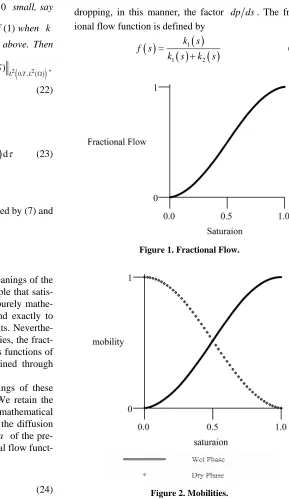
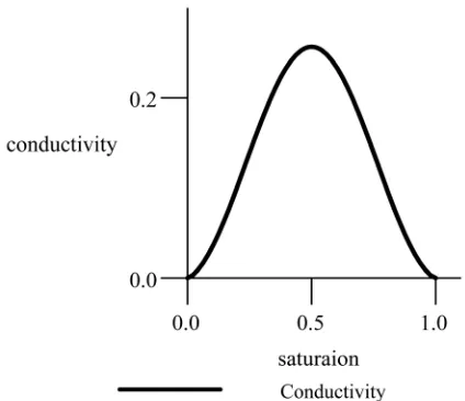
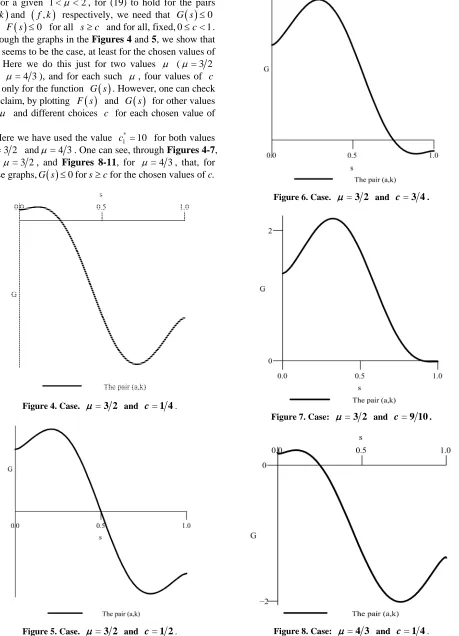
In this Section, we describe the physical meanings of the parameters in Problem 1 and give an example that satis- fies conditions (2) through (3). These are purely mathe- matical examples that might not correspond exactly to models derived through physical experiments. Neverthe- less, the shapes of the graphs of the mobilities, the fract- ional flow function, and the conductivity, as functions of the saturation , resemble the ones obtained through experiments. See Figures 1-3, for
S
= 3 2
.
For more details on the physical meanings of these parameters, see [1,2,10-12], for instance. We retain the simplicity of the examples below for the mathematical analysis in this paper. For these examples, the diffusion coefficient (also called the total mobility) of the pre- ssure equation of (1), as well as the fractional flow funct- ion,
a
f , satisfy (5). Physically
= 1
2
a s k s k s (24)
where 1 is the mobility of the wetting phase, and the 2 the mobility of the nonwetting phase. The con- ductivity of the porous medium is defined by
k k
1
2
1 2
d =
d
c
k s k s p
k s
k s k s s , (25)
where pc is the capillary pressure. Assuming dpc ds
is bounded and bounded away from 0, we will define, for this analysis,
1
2
1 2
= k s k s
k s
k s k s , (26)
dropping, in this manner, the factor dp ds. The fract- ional flow function is defined by
1
1 2
= k s
f s
k s k s (27)
[image:4.595.234.523.224.723.2]Figure 1. Fractional Flow.
Figure 3. Conductivity of the Medium.
and a, the total mobility, is given by (24).
For numerical modeling of immiscible two-phase flow through porous media, it has been used the following mobilities (see [13], for example).
1 =
k s s (28) for the wetting, and
2 = 1k s s (29) for the nonwetting phase, up to multiplicative constants (or bounded functions). For a mathematical analysis purpose, and in order to get an example of uniqueness of a solution of Problem 1, we multiply both (28) and (29) by a bounded function of
s
on the interval
0,1 . 4.1. A case of UniquenessWe define our new mobilities (up to the same multipli- cative constant) by the following. For 1 <2
, let
21 = e ,
s s
k s s (30) for the wetting phase, and
22 = 1 e ,
s s
k s s (31) for the non wetting phase. Then, the total mobility (up to a multiplicative constant K, the absolute permeabi- lity, which we take here to be 1) is given by
2= 1 e s s
a s s s , (32) while the conductivity of the medium (up to the same multiplicative constant K) is given by
2
1 e
= ,
1
s s
s s
k s
s s
(33)
and the fractional flow function is given by
=1
s
f s .
s s
(34) It is clearly seen that , defined by (26), satisfies (2) and (3), and that
k
f and satisfy (5) for a 1 <2. One also checks that if = 2, then
2
2 0, 1 0, 1 .
L L
a f C (35)
Therefore, for k defined by (33), f defined by (34), and a defined by (32), we have that the couple
a k, and
f k,
satisfy (6), by Lemma 2.1 and Lem- ma 2.2. Hence the following.Corollary 4.1 Under the conditions (26) through (34), if = 2, Problem 1 has a unique solution . Fur- thermore, the family of regularized solutions
p S,
p,S
, as defined by Theorem 3.2, converges to the unique solution
p s, of (1).Conditions (32) through (35) and Corollary 4.1 show that condition (9) is not empty, neither is condition (6), which is often used in the proof of the well-posedness of problem 1 or the like and for the convergence of the re- gularization of the same type of problems ([3,4,6,7,14]. 4.2. Graphical Experiments for Uniqueness
One can check, through computations, that a and f , as defined by (32) and (34), respectively, are not twice continuously differentiable, for 1 << 2. They fail to be twice differentiable at s= 0 and s= 1. For some values of ,1 << 2, namely for the values = 3 2 and = 4 3, we show graphically, experimenting with several values of , that condition (19) seems to hold for and
c
a f defined by (32) and (34). So this is an indication that Corollary 4.1 could hold for these values of (and, maybe, for 1 << 2). We emphasize that this does not constitute a rigorous mathematical proof that Corollary 4.1 holds for these values of , but it does point to the conjecture that this could be the case.
For our graphical illustrations, we define the functions
G s and F s
on the interval
0, 1 , for a given 1 << 2 by,
*
1 :
= G s
a s a s a c c k s s c K s K c
(36) and, in the same way,
*
2 :
= ,
F s
f s f s f c c k s s c K s K c
(37) for a parameter 0 c 1. Here and are fixed positive constants that are independent of , but could depend on
* 1
c *
2
c c .
For a given 1 << 2, for (19) to hold for the pairs and
a k,
f k,
respectively, we need that G s
0 and F s
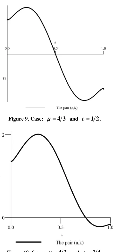
0 for all sc and for all, fixed, 0c< 1. Through the graphs in the Figures 4 and 5, we show that this seems to be the case, at least for the chosen values of . Here we do this just for two values (= 3 2 and = 4 3), and for each such , four values of and only for the function . However, one can check our claim, by plottingc
G s
F s and for other values of
G s
and different choices c for each chosen value of .
Here we have used the value 1 for both values *
= 10
c
= 3 2
and= 4 3. One can see, through Figures 4-7, for = 3 2, and Figures 8-11, for = 4 3, that, for these graphs,G s
0forscfor the chosen values of c.Figure 4. Case. =3 2 and c=1 4.
Figure 5. Case. =3 2 and c=1 2.
Figure 6. Case. =3 2 and c=3 4.
[image:6.595.72.531.83.719.2]Figure 7. Case: =3 2 and c=9 10.
Figure 9. Case: =4 3 and c=1 2.
Figure 10. Case: =4 3 and c=3 4.
Figure 11. Case: =4 3 and c=9 10.
4.3. Other Graphical Experiments for Uniqueness for 1<
<2In this subsection, we use other arguments to show that the hypotheses of Lemma 2.1 seem to hold for the fun- ctions a and f , respectively, for 1 << 2. We con- sider the following functions.
, :=
f
x
f x
f y
, F x yk x x y K x K y
(38) and
, :=
a x
a x
a y
. (39) G x yk x x y K x K y
Clearly, condition (9) holds for f and a, if the fun- ctions F and , defined respectively by (38) and (39) are bounded above independently of
G
x and on the region enclosed by the triangle with vertices (0,0), (1,0), and (1,1) i.e. the region
y
2
, := , x>y
R x y 0, 1
R
. Notice that the common denominator of both functions is positive in the interior of the region . See Figure 12 below.
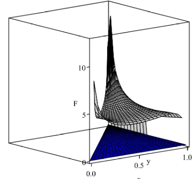
Functions F and G are very complex by their defi- nition, especially for non integer values of . They in- volve the integral-defined function K. They e diffi- cult to handle algebraically. For the present work, we sketch the surfaces representing the two functions, above the region R, for some valu of
ar
es , using Maple So - ware, in order to analyze their boundedness. This is illu- strated through the Figures 13through 18.
We notice
ft
the smoothness of the surfaces correspond- ing to the case = 2. This suggests that the two funct- ions are definitely bounded in this case. For = 2, we show directly that this is indeed the case that Corollary 4.1 holds. We prove this through the following lemma.
Lemm
, i.e.
a 4.2 For = 2, functions F and , defined
by tiv
G
(38) and (39), res ely, are bounded indepen- dently of
pec
x y, over the region R.Proof of Lemma 4.2. From (32) and (34), it is easily se
en that
1 1
2
1 =
1
x x
f x
x x
(40)
and
2
2 2
=
1 1 2 1 2 3 x x
x x x x x x e
.
(41) s
a x
[image:7.595.80.269.71.490.2]Figure 12. Region R.
[image:8.595.324.507.298.493.2]Figure 13. Surfacez=F x y , over region R, for
,
=3 2.Figure 14. Surfacez=G x y
,
xFigure 15. Surfacez=F x y , over region R, for
,
=4 3.
= ,
z G x y
over region R, for =3 2.
Figure 16. Surface , over region R, for=4 3.
= ,
z F x y =2.
[image:8.595.331.511.516.709.2] [image:8.595.75.270.519.699.2]Figure 18. Surface z=G x y , over region R, for
,
=2.On the other hand, by the Mean-Value Theorem, we have
1
2, = f x f x y = f x f
F x y
k x x y k x y k x k
1
2
(42) and
3
4, = a x a x y = a x a
G x y
k x x y k x y k x k
3
4
(43) where i, 1 i 4, are between x and and where
we have obtain from an ) that y, d (43 used (7). We (42)
12 2
f x f
y
k ,
F x
x k
(4
an
4)
d
34 ,
2 a x a G x y
k x k
(45
Combining (33),(40), (41), (44), and (45), we obta )
in
1
12 2
, = 1
F x y O x x
(4 ) and
6
1
12 2
=O x 1 ,
(47) ,
G x y x
as yx, y<x. Hence, if = 2, F x y
, and
,G x y are bounded on . Th
Conjecture. Corollary 4.1 also holds for
R is proves the lemma. 3
< 2 2 .
hope, in a future work, to be able to prove this claim or give a counterexample that disproves it. If this claim happens to be true, that would
functions and We
give examples of
a f
que
that are not very smooth but for which the s uni ness for the problem (1).
5. Conclusions
In this paper, we have revisited the problem of unique- r the pressure/saturation system. A new sufficient condition for uniqueness has been established and we have showed that the old conditions for un
ditions (3), (5), and (35)) imply the new condition. An mple of famil nding n a param
re i
ness fo
iqueness (con-
exa a y of data (depe o eter
) has
been constructed that gives uniqueness for = 2
. For the general case 1 << 2, we have illustra- ted graphically (without a rigorous proof) that there co
e
[3] K stence an
ysis, Vol. 5, 2001, pp. 503-521.
“Regularization and Numerical Methods Porous Medium Equations,” PhD Thesis, University of South Carolina, Columbia, 1993.
uld be uniqueness for these cases. A sequel of this paper should concern itself with a rigorous proof (or dis- proof) of this claim. It should also concern itself with the general cas , especially the case of convection domina- ted flow.
6. References
[1] G. Chavent and J. Jaffre, “Mathematical Models and Finite Element for Reservoir Simulation: Single Phase, Multiphase and Multicomponent Flows through Porous Media,” North-Holland,New York, 1986.
[2] R. E. Ewing, “Problems Arising in the Modeling of Processes for Hydrocarbon Recovery,” In R. E. Ewing, Ed., The Mathematics of Reservoir Simulation, S.I.A.M., Philadelphia, 1983, pp. 3-34.
. B. Fadimba, “On Exi d Uniqueness for a Coupled System Modeling Immiscible flow through a Porous Medium,” Journal of Mathematical Analysis and Applications, Vol. 328, No. 2, 2007, pp. 1034-1056. doi:10.1016/j.jmaa.2006.06.012
[4] Z. J. Chen and N. L. Khlopina, “Degenerate Two-Phase Flow Problems: Error Estimates,” Communication in Ap-plied Anal
[5] K. B. Fadimba, for a Class of
[6] K. B. Fadimba and R. C. Sharpley, “A Priori Estimates and Regularization for a Class of Porous Medium Equa-tions,” Nonlinear World, Vol. 2, 1995, pp. 13-41. [7] Z. Chen and R. E. Ewing, “Degenerate Two-Phase
In-compressible Flow-III: Sharp Error Estimates,” Numeri- sche Mathematik, Vol. 90, No. 2, 2001, pp. 215-240. doi:10.1007/s002110100291
[8] K. B. Fadimba and R. C. Sharpley, “Galerkin Finite Ele-ment Method for a Class of Porous Medium Equations,” Nonlinear Analysis: Real World Applications, Vol. 5, No. 2, 2004, pp. 355-387. doi:10.1016/j.nonrwa.2003.07.001
s for Flows through
Po-ater Flow and
umerical
a, “Computational Methods
mylie, “A near Optimal Order Approximation to a
eak Solu-[9] M. E. Rose, “Numerical Method
rous Media-I,” Mathematics of Computations, Vol. 40, No. 162, 1983, pp. 437-467.
[10] J. Bear and A. Verruijt, “Modeling Groundw
Pollution,” D. Reidel Publication Company, Dodreich, 1987.
[11] R. E. Ewing and H. Wang, “A Summary of N Methods for Time-Dependent Advection Dominated Par-tial DifferenPar-tial Equations,” Journal of Computational
and Applied Mathematics, Vol. 128, No. 1-2, 2001, pp. tion 423-445. doi:10.1016/S0377-0427(00)00522-7
[12] Z. Chen, G. Huan, and Y M
for Multiphase Flows in Porous Media,” SIAM Computa-tional Science and Engineering, Philadelphia, 2006. [13] D. L. S
Class of Two-Sided Nonlinear Parabolic Partial differen-tial Equations,” PhD Thesis, University of Wyoming, Laramie, 1989.
[14] Z. Chen, “Degenerate Two-Phase Incompressible Flow-I: Existence, Uniqueness, and Regularity of a W