On the Thermodynamical Black Hole Stability in the Space Time of a Global Monopole in f(R) Gravity

(1)

http://www.scirp.org/journal/jhepgc ISSN Online: 2380-4335 ISSN Print: 2380-4327

DOI: 10.4236/jhepgc.2019.53032 May 10, 2019 587 Journal of High Energy Physics, Gravitation and Cosmology

On the Thermodynamical Black Hole Stability

in the Space-Time of a Global Monopole in

f

(

R

)-Gravity

Francisco Bento Lustosa

1*

_{, Maria Emilia Xavier Guimarães}

2

_{, Cristine Nunes Ferreira}

3

_,

Joaquim Lopes Neto

4

, José Abdalla Helayël-Neto

5

1_{Departamento de Fsica Teórica, Instituto de Fsica, Universidade do Estado do Rio de Janeiro, Rio de Janeiro, Brazil} 2_{Instituto de Fsica, Universidade Federal Fluminense, Campus da Praia Vermelha, Niterói, Brazil}

3_{Núcleo de Estudos em Fsica, Instituto Federal de Educação Ciência e Tecnologia Fluminense, Rio de Janeiro, Brazil} 4_{Instituto de Fsica, Universidade Federal do Rio de Janeiro, Rio de Janeiro, Brazil}

5_{Centro Brasileiro de Pesquisas Fsicas, Rio de Janeiro, Brazil}

Abstract

In this work, we re-assess a class of black hole solutions in a global monopole spacetime in the framework of an

f R

( )

-gravity model. Our main line of in-vestigation consists in considering a region close enough to the black hole, but such that the weak field approximation is still valid. The stability of the black hole is studied in terms of its thermodynamical properties, with the radial coordinate written as a power-law function with the status of the main factor underneath the stability of the model. We obtain the explicit expressions for the thermodynamical quantities of the black hole as functions of the event horizon, by considering both the Hawking and the local temperatures. The phase transitions that may occur in this system, including the Hawking-Page phase transition, are inspected with particular attention. We work out and con-template a solution of special interest in which one of the parameters is related to the cosmological constant. Our main result sets out to establish a compar-ison between both the Hawking and the local formalisms for the black hole in the framework of the

f R

( )

-gravity in the particular space-time adopted here.

Keywords

Black Hole, f(R)-Gravity, Hawking Temperature, Global Monopole, Cosmological Constant

1. Introduction

There are still some important issues for which current cosmological standard How to cite this paper: Lustosa, F.B.,

Guimarães, M.E.X., Ferreira, C.N., Neto, J.L. and Helayël-Neto, J.A. (2019) On the Thermodynamical Black Hole Stability in the Space-Time of a Global Monopole in f(R)-Gravity. Journal of High Energy Phys-ics, Gravitation and Cosmology, 5, 587-611. https://doi.org/10.4236/jhepgc.2019.53032

Received: March 6, 2019 Accepted: May 7, 2019 Published: May 10, 2019

http://creativecommons.org/licenses/by/4.0/

(2)

DOI: 10.4236/jhepgc.2019.53032 588 Journal of High Energy Physics, Gravitation and Cosmology theories in Physics have not yet found complete answers. General Relativity (GR) has not been able to clarify questions such as the non-renormalization of the gravity theory, the singularity problems in black hole physics and the physics of the early Universe, leading us to the necessity of finding alternative approaches. In this context, one of the most intriguing facts is the accelerating Universe. De-spite of the existence of some alternative approaches to explain this behavior, one of those without adding dark matter or dark energy [1] [2] [3], and the other with

f R

( )

gravities [4] [5] that has received much attention as one of the strongest candidates to explain the current accelerating universe [6]. The

f R

( )

gravity is constructed by replacing the Ricci scalar in the Einstein-Hilbert action by an arbitrary function of the Ricci scalar

f R

( )

. Such theory is well known to lead to an extra scalar degree of freedom and it has been shown, for example in

[7] [8] [9], that observationally acceptable models may be built up. In some new contributions,

f R

( )

-gravity can exhibit dependence on higher powers of the curvature scalar [10].

In 1972, Bekenstein published his first article demonstrating the relation be-tween thermodynamic quantities and gravitational properties of a black hole. His works [11] [12] [13] [14] were followed by the model of particle creation around BH proposed by Hawking [14]. Since then, the thermodynamical beha-vior of quasi-classical systems has been widely explored in other gravitational frameworks. Most recent contributions were made in the study of the thermo-dynamics of the black hole in modified Schwarszchild [15], Born-Infeld-anti-de Sitter [16], Horava-Lifshitz [17], torsion [18] and

f R

( )

theory [19].

It has been shown that topological defects such as cosmic strings, monopoles and domain walls could be formed as a result of spontaneously broken symme-try in a vacuum phase transition of the early universe [20] [21]. In the context of the GR, Barriola and Vilenkin [22] studied the gravitational effects of a global monopole as a spherically symmetric topological defect. In the context of

f R

( )

-theories, global monopoles heve been recently studied by [23] [24] [25] [26], and references therein. In this solution, there appears a term which corresponds to a black hole solution. It is natural, then, to imagine that there is a region with a global monopole that could have been swallowed by a black-hole. Another inter-esting situation where the monopole appears as an important ingredient involves boson stars. When these compact objects are present along with a non-minimally coupled global monopole, a black-hole-type solution can be mimicked. This ap-proach is important to unveil the non-linear gravitational effects and the gravi-tational back reaction [24].

On the other hand, the analysis of the thermodynamical properties of that case, in the context of GR, was carried out in [27] and, more recently, in the context of an

f R

( )

-theory in [28], where the authors adopt the weak field ap-proximation solution presented in [23] with a specific ansatz for

( )

d

( )

d

f R

f R F R

R

(3)

DOI: 10.4236/jhepgc.2019.53032 589 Journal of High Energy Physics, Gravitation and Cosmology as a linear function of the radial coordinate.

In the present paper, we consider thermodynamical aspects of black holes in the space-time of a global monopole in the framework of

f R

( )

-gravity. We study a general case in which

f R

( )

is a power law function of the radial coor-dinates. We anticipate that we obtain the explicit expressions for the local ther-modynamical quantities of the black hole as a function of the event horizon, the parameter describing the monopole and the measurable corrections on the usual GR gravity due to the

f R

( )

-extension.

Our work is organized according to the following outline: In Section 2, moti-vated by the analysis of thermodynamic aspects, we revise the solution for a black hole in the region containing a global monopole with the use of a

f R

( )

-model; the investigation is pursued by adopting the weak field approximation

[26]. The new result in this section is the ψ <n 0-case. Section 3 is split into

subsections. In the first part, we analyze the entropy expression taking into ac-count the corrections inherent to the case of an

f R

( )

-theory. The stability of the black hole is also contemplated—in the Hawking’s approach—by taking into account the positivity of temperature and specific heat. In Part B, the black hole stability is re-assessed by following an alternative treatment. In part C, one stu-dies the phase transitions of the system and a comparison is established between the Hawking’s and the local case approaches. Finally, in Section 4, we cast our Closing Remarks and present, more carefully, a discussion on the particular n = 2-case; in this special case, the ψ2-parameter is related with both situations of a

positive and a negative cosmological constant that, in the presence of the global monopole, exhibits a solid angle deficit.

2. Field Equations Solution for the

f

(

R

) Gravity in the Metric

Formalism: A Review

In this section, for the sake of understanding, we make a small review of the so-lution of the field equations for an

f R

( )

-theory with a spherically symmetric space-time obtained in [26]. In this reference it is shown that it is possible to find a black hole solution in a global monopole region by using an

f R

( )

mod-ification of the GR gravity within the weak field approximation. For an

f R

( )

theory, the action associated to the matter field coupled with gravity is given by:

( )

(

)

4

1

d , ,

2 m

S= _κ

∫

x −g f R +S gµν ψ (1)

where κ=8πG, G is the Newton constant, g is the determinant of the metric

(4)

DOI: 10.4236/jhepgc.2019.53032 590 Journal of High Energy Physics, Gravitation and Cosmology + 3) dimensions is given by

( )

(

)

2 2 2 2 2 2 2

ds =B r dt −A r dr −r dθ +sin θ φd (2) The g_µν field equations read as below:

( )

1

( )

(

)

( )

2

R F R_µν − f R g_µν − ∇ ∇ −_µ _ν g_µν F R =κT_µν (3) with

( )

d

( )

d

f R F R

R

= _{, and} is the usual notation for covariant D’Alembert

operator µ

µ ≡ ∇ ∇

 . The only term associated to the matter action is related to the global monopole described by the Lagrangian density

(

)(

)

(

₂

)

2

1 1

,

2 4

a a a a

L= ∂µφ ∂µφ − λ φ φ −η (4)

where λ and η are the monopole field parameters and the triplet field that will result in a monopole configuration that can be described by

( )

2

a h r a

x r

φ

=

η

_,

with a=1, 2, 3 and a a 2

x x =r . The function

h r

( )

is dimentionless and is constrained by the conditions

h

( )

0 =

0

and

h r

(

>

η

)

≈

1

[22]. The ener-gy-momentum tensor associated with that field configuration is

2 2

0

t r

T T

r Tθθ Tφφ

η

= ≈

= =

(5)

We can now focus on the gravitational effects of the global monopole in the

( )

f R

approach to gravity, by taking the trace of the field Equation (3) in the presence of the monopole [23] [25]

( )

1

( )

3

( )

2 2 2

f R = RF R + F R −κT (6) where

( )

d

( )

d

f R F R

R

= _{. By replacing (6) in (3), we have}

( )

F R R

µν

− ∇ ∇

µ ν

F R

−

T

µν

=

g C

µν (7) where the quantity 1

(

( )

)

4

C= F R R−F R −κT is a scalar quantity.

In a spherically symmetric space-time, with the metric given by (2) and with the energy-momentum tensor expressed by (5), we find, by virtue of (7), that the equations may be written as

(

)

2 rF

′′

−

β

rF

′

+

2 F

=

0,

(8)

(

)

(

)

2 4

4B A 1 r 2F rB 2B 2r B AB 0

F F

α

β

′

  _′ _′′

− + _ − _ − + − =

  (9)

where α_and β are:

2

2 , with

8π

G

α

=

κη

κ

=

₍₁₀₎

( )

.

AB

(5)

DOI: 10.4236/jhepgc.2019.53032 591 Journal of High Energy Physics, Gravitation and Cosmology We make the assumption of time-independent solutions, i.e.

B

=

B r

( )

and

( )

A

=

A r

, which yields the metric as given in (2). With these assumptions, we consider

F R

( )

=

F r

( )

and F′ and F′′ are the first and the second deriva-tives with respect to r, respectively. The solution to these equations is the exact description of the global monopole in

f R

( )

theories. This prescription has however an analytical solution only in the weak field approximation. In this ap-proximation, the field equations read as follows:

( )

1 ( )

F R

=

F r

= +

ψ

r

( )

1 ( ) ( )

,

1 ( )

B r

= +

b r

A r

= +

a r

(12) with b r

( )

, a r

( )

and ψ

( )

r much smaller than one. These redefinitions are used in Equation (8) and Equation (9), and with the help of

,

F F

F ψ F ψ

′ _′ ′′ _′′

  (13)

,

A B

a b

A B

′ ′

  (14) the field Equation (8) and Equation (9) can then be written in a linear form as:

( )

,

r

β



ψ ′′

(15)

( )

2

( )

2

2a r −2r

ψ

′ r +r

β

+r b r′′ −2

κη

=0, (16)

where β has been defined in (11). This is the solution to our equations in the weak field approximation for a metric with spherical symmetry in an

f R

( )

-theory with d

( )

1

( )

d

f R

r

R = +

ψ

where R is the function of the radial coordinate,

r. Following in [26], we assume that the function

ψ

( )

r

is a power law-like function of the radial coordinate, namely

ψ

( )

r =

ψ

( )nrn, where ψn is a

con-stant parameter in r. Notice, however, that in our work it shows a dependence on n. With this ansatz, we can find solutions for the equations above. Noting that Equation (11) with Equation (14) can be rewritten as:

( )

(

)

( 1) 1 _n n

a r′ +b r′ =n n− ψ r − (17) we can solve (16) for

b r

( )

, obtaining:

( )

1 n 2_.

n

c

b r r

r ψ κη

= − − (18)

We define the integration constants c1= −2GM and, for convenience, we

take c2 =0. This term corresponds to the cosmological constant term. Equation

(11) and Equation (15) yield the relation:

( ) ( )

( )1

0e .

n n

n r

A r B r =a −ψ (19) Defining the integration constant a0 =1, we then have the full form of the

me-tric as

( )

( )1

_{( )}

1

2 2 2 2 2

(6)

DOI: 10.4236/jhepgc.2019.53032 592 Journal of High Energy Physics, Gravitation and Cosmology

( )

₁ 2 2 n

n

GM

B r r

r

κη ψ

= − − − (21)

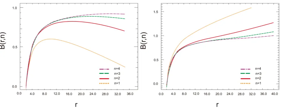
In Figure 1, we plot the function

B r n

( )

,

for n varying from 1 to 4. It can be seen, in the case of the figure on the left, with ψ >n 0, that the function

B r n

( )

,

grows to a value and then decreases for all orders of n. In the case ψ <n 0, the

function transits to ever increasing values.

Considering the mass term as cosmologically relevant is equivalent to adopt-ing the scenario with a black hole in the space-time of a global monopole [22]. To confirm that our solution is actually a black-hole-type solution for all degrees n of the

ψ

( )

r

-function, we have to find if all of them have an event horizon. To do this, we have to keep in mind the approximations that we have used to solve the field equations, namely h≈1, which we have employed to define the

ener-gy-momentum tensor outside the core of the global monopole, and ψ

( )

r 1. These approximations require that we restrict our analysis to a region defined by:

1 n n

r r δ

ψ

< < (22)

where δ_≈

(

λη1 2

)

is the order of magnitude of the monopole’s core.

In the following sections, we shall concentrate on the cases where ψ <n 0

and ψ >n 0 in the limit given by (22). These solutions do not contemplate the

asymptotic case when n>0; however, its analysis is important if we wish to consider regions closer to the black hole.

3. The Thermodynamics of the Black Hole in an

f

(

R

) Global

Monopole for Generic

n

[image:6.595.65.537.504.687.2]

In this section, the thermodynamic behavior is reported for two cases. In one of the cases, with ψ <0, the stability of the BH is ensured for all powers; the other

Figure 1. Graphs for B(r, n) in function of position for each n-orders going from 1 to 4, where GM=1 and 2 5

0.3 10

κη ₌ _× − _{. In}

the figure (a) 2

0.2 10 n n

ψ ₌ _× − _{and (b)} 2

0.2 10 n n

(7)

DOI: 10.4236/jhepgc.2019.53032 593 Journal of High Energy Physics, Gravitation and Cosmology case, where ψ >0, the technique of local thermodynamics has been adopted to analyze the stability of the BH.

3.1. The Hawking Thermodynamics and the Power Law Series for

a Generic

n

In this sub-section, we shall be considering the thermodynamical behavior of a black hole in a region with a topological defect, by following the Hawking pro-cedure. We can analytically with prove that the metric has an event horizon for the solution of an

(

n

+

1 )

-degree equation:

2 2

1 _{n H}n 0.

H

GM r r

κη ψ

− − − = ₍₂₃₎

We have written the parameter ψn as a power law-like function of radial

coordinate for a generic n. This is essential to respect the condition (22) without narrowing the region that we are going to analyze. Considering only the region where ψ

( )

r 1 implies that the other roots of Equation (23) are out of the region where our solution is valid. In addition to the limit for ψn and

2

κη

_,

used in the previous graphs, the black hole (BH) stability was analyzed in detail considering the functions of temperature, heat capacity and its phase.

From (23), we get the dependence of the energy (GM) on the horizon rH

(

2

)

1

1 1 2

n

H n H

GM = _ −κη r −ψ r + _ (24)

The Hawking temperature can be readily obtained from the GM expression, which corresponds to the energy of the black hole. The Hawking temperature is, therefore, the derivative of the energy with respect to the entropy of the black hole [29]

( )

1

(

)

2

4 1 ,

4

n

n H H

S =F R A ≡ +ψ r πr (25)

where A is the area of the event horizon.

In Figure 2, which shows graphically the behavior of the entropy with the ra-dius of the horizon, it indicates that there are critical points for different values of n given by the expression to rH:

(

)

(

)

max

1 1

2 n 2 n

H n

r = −ψ n+ − (26) In this expression it can be easily verified that

r

Hmax applies only when ψ <0,

as can be seen by the graphs of Figure 2. This fact has given us an important sult which was related to the critical range between allowed and forbidden re-gion, but throughout this work will be analyzed if this transition is within the limit of validity of the solution found.

(8)

[image:8.595.85.537.60.269.2]

Figure 2. Graph for S r

( )

H for n going from 2 to 4 and Schwarzschild black hole with global monopole,

2 5

0.3 10

κη ₌ _× −

where in left panel 2

0.4 10 n n

ψ ₌ _× − _{and in the right panel} 2

0.4 10 n n

ψ _{= −} _× − _.

Figure 3. Graphs for GM_HW

( )

S n, for n going from 2 to 4 and the Schwarzschild black hole case, 2 5

0.3 10

κη ₌ _× − _and 2

0.4 10 n n

ψ _{= ±} _× − _.

in fact to its entropy and consequently, its superficial gravity is responsible for measuring the temperature that the radiation emitted by the black hole will have. Although we are far from testing these results experimentally, the apparent lack of inconsistencies in the theoretical model and its application to several cases of interest [4] make it widely accepted.

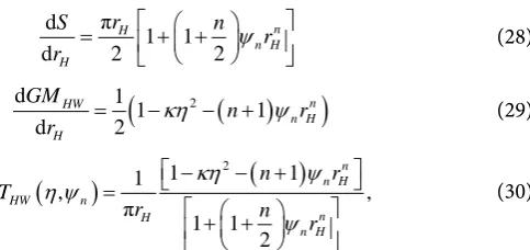
The prescription for the Hawking’s temperature is given by the second low d

d

GM T

S

= _{given by}

1

d d

HW

H H

GM S

T

r r

−

 

= _ _

[image:8.595.91.535.321.519.2]

(9)

DOI: 10.4236/jhepgc.2019.53032 595 Journal of High Energy Physics, Gravitation and Cosmology where

π d

1 1

d 2 2

n H

n H H

r

S n

r

r ψ

   

= _ + +_ _ _

 

  (28)

(

)

(

2

)

d 1

1 1

d 2

n HW

n H H

GM

n r

r = −κη − + ψ (29)

(

)

1 1 2

(

1

)

, ,

π ₁ ₁

2

n n H

HW n

n H

n H

n r

T

r n

r

κη ψ

η ψ

ψ

 − − + 

 

=

 _{+ +}  

 

 _ _ 

 

(30)

which, for n=1, recovers the result obtained in [28], and, for η=0,

ψ

( )

r

=

0

, the Schwarzschild result is reproduced. In this work, we concentrate in the case

1

[image:9.595.295.537.88.202.2] [image:9.595.240.506.449.671.2]

n> with a Schwarzschild-like solution in presence of a global monopole.

Figure 4 shows that, for all values of n, there are two types of the black hole temperature: one with the temperature decreasing with the horizon, rH, and the

other with the temperature growing with the horizon. The minimum point be-tween these two regimes is calculated in this model by the derivative of the Hawking temperature as a function of the horizon radius d HW 0

H

T

r = . The expression resulting from this calculation is a simple polynomial of degree n, for

1

n≠ . In this graph it can also be seen that the temperature behavior in this re-gion has the same shape and transition. This fact has not been applied to the whole region of space.

Despite the positivity of the temperature, to analyze the stability of the black hole, it is necessary to verify the prescription for the heat capacity. Using the

Figure 4. Graph for the Hawkings temperature, T in function of the horizn radio rH,

with 2 5

0.3 10

κη ₌ _× − _and_n_{going from 2 to 4, with Schwarzschild black hole with global}

monopole 2

0.4 10 n n

(10)

DOI: 10.4236/jhepgc.2019.53032 596 Journal of High Energy Physics, Gravitation and Cosmology laws of thermodynamics for black holes, it has been found that it is possible to obtain the heat capacity of the black hole by considering the entropy of the sys-tem, i.e. dE=T Sd . In the case where the volume is constant, the energy, E, can

be related to the mass of the black hole.

We shall now look for the heat capacity, which can be calculated from the energy. The expression is obtained as follows:

1

d d

d

d d d

H H

HW

H r H H

r

GM T

GM C

T r r

−

 

  _   _

=_ _ = ⋅_ _

 

  _   _ (31)

(

)

(

2

)

d 1 1 1 d 2 n H H H GM

u n r

r κη ψ

= = − − +

(

)

₍

₎

(

)

2 2

2 2 2

d 1

d

4π 1 1 2

1 2

1 1 1 1

1

H

H n

n H H

n n

n H n H

T v

r _n

r r

n

n r r

n

ψ

κη κη ψ ψ

= = −  _{+ +}      _ _       ₊           _   _  × −_ + − + − − _ −        _ _    H u C v

= (32)

By considering Equation (30) and Equation (24), we obtain the expression:

(

)

(

)

₍

₎

(

)

2

2 2

2

2 2 2

1 1 1 1

2 2π

1 2

1 1 1 1

1

n

n H n H

HW H

n n

n H n H

n

n r r

C r

n

n r r

n

κη ψ ψ

κη κη ψ ψ

     − − + _ + +_ _ _  _ _ _ _ = −   ₊      _ _    − + − + − − −       (33)

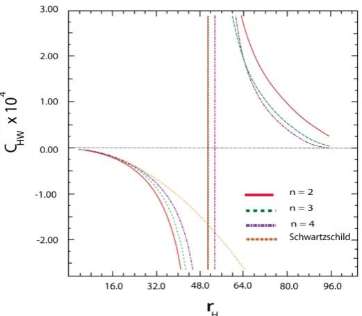
In Figure 5, we see the heat capacity plotted for the classical case and the 2

n= to 4 and compared with the Schwarzschild black hole.

By inspecting Figure 4 and Figure 5, one can discuss the validity regions of our solution of the BH in terms of the temperature and heat capacity. It can be seen that, for the region *

H H

r

δ ≤

<

, the temperature is positive but the specific heat is negative. This region is therefore prohibited because it has a negative heat capacity because it is not in accordance with the laws of thermodynamics. There is a discontinuity in the heat capacity equation at the point *

H H

r

=

r

, which can be seen in the graph of Figure 5. This discontinuity is the point where the spe-cific heat changes behavior, becoming positive. In this region both temperature and heat capacity are positive, with the possibility of obtaining an allowable so-lution for the black hole.

Due to the maximum point given by the Equation (26) and which can be seen graphically in Figure 2, we have another phase transition in this system. For

max H

(11)

[image:11.595.244.505.73.300.2]

Figure 5. Graph for heat capacity, C, with 2 5

0.3 10

κη ₌ _× − _with 2

0.4 10 n n

ψ _{= −} _× − _and

panel right.

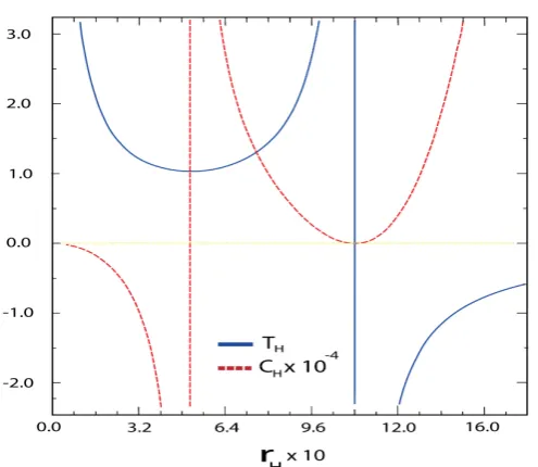
horizon, to increasing with the radius of the horizon, and this destabilizes the BH presenting negative temperatures, in this way this region becomes forbidden as we can saw in Figure 6. In the next section we will discuss the local case, where we will compare the local temperature with the Hawking temperature, this comparison gives us new results.

In the graph of Figure 6 it is easy to see that the transition is located exactly at the maximum point of the entropy curve given by the expression (26).

It may be verified that, whenever ψ >n 0, both regions are prohibited,

be-cause, for a positive temperature, the heat capacity is negative, and when the heat capacity is positive, the temperature is negative. Then, in the case of

0

n

ψ > _{it is necessary to work with another prescription that, in this paper, we} take as the local prescription.

3.2. The Local Thermodynamics of the Black Hole for a Generic

n

In the previous section, we have treated the thermodynamical properties by con-sidering the Hawking formalism, where it is possible to investigate the properties in the case ψ <n 0. In the present section, we go through a formulation where it

is possible to discuss the stability conditions independently of the signal ψn. We

(12)

[image:12.595.252.500.65.280.2]

Figure 6. Graph for temperature and heat specific, C in function of the horizon ratio for

n = 2, with 2 5

0.3 10

κη ₌ _× − _and 2

0.4 10 n n

ψ _{= −} _× − _.

be derived. We use the prescription given in [32] to obtain the local temperature of the black body radiation:

00

loc

T T

g

= (34)

with this relation the temperature was obtained as a function of the position as

(

)

(

) (

)

2

1

1 2 2 1

1

1 1

π

1 1

2

1 8π 1 8π

n n H H

loc

n n H

n n

n H H n

n r

r T

n r

r

r r G r G r

κη _ψ

ψ

ψ η η ψ

−

+ +

 − ₋ ₊ 

 

 

=

 _{+ +}  

 

 _ _ 

 

×

− − + − −

(35)

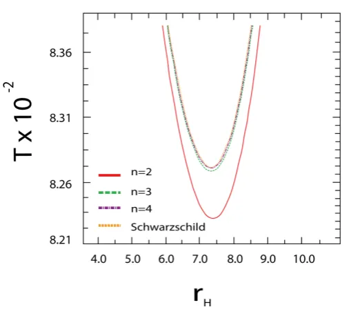
The local temperature for n=2 to 4 and the Schwarzschild black hole is plot-ted in Figure 7 as a function of the event horizon where we fixed the position at

10

r= . The graph is zoomed to show the slight variation difference between the minimum values of the temperature for different values of the degree n.

An important characteristic to observe at this temperature is the existence of a minimum in its variation with respect to the event horizon. This minimum can be called the critical temperature [33], which would be the minimum tempera-ture in the region around the black hole. In Figure 7 the local temperature curves for n = 2, 3, 4 and the Schwarzschild were calculated numerically. Dis-plays that, for all values of n, there are two possible black holes: one for which the temperature diminishes with the horizon, to *

H H

r

>

r

, and the other with the temperature growing with the horizon, to rH >rmin. These phase transitions

(13)

[image:13.595.247.499.65.294.2]

Figure 7. Graph for Tloc

( )

rH for n=2,3, 4 and Schwarzschild, for r=10.

It is important to notice, from this and the following graphs, that we fix a po-sition for the measurement of the temperature and we are analyzing how the temperature in that position varies as the event horizon increases. That means, we are finding what size the black hole has at the moment in which the temper-ature in the position r = 10 is minimal. In this sense, we see that as the horizon approaches the chosen position the temperature decreases rapidly to the mini-mum and then increases asymptotically when it approaches r = 10.

From the first law of thermodynamics dGMloc =TlocdS, the thermodynamical

local energy, GMloc, can be derived. Following the prescription discussed in last

section, we can assume that

( )

1

(

)

2

4 1 π

4

n

n H H

S=F R A ≡ +ψ r r , where A is the area of the event horizon.

( ) ( )

_{( )}

0

0 0 ₀

π

d 1 1 d

2 2

H

S r M _n

loc _S loc _r _M loc n

n

GM =E + T S=E + ₌ T ξ _ + +_ _ψ ξ ξ ξ_

 

 

∫

(36)

where we choose E0 =0 for simplicity. Using the expression for the local

tem-perature in the integral using

(

)

(

)

1

2

0 1

n

H n

r M= =_ −κη ψ _− (37) with the integration constants conveniently, we get

(

)

(

) (

)

2

2 2

1 8π

1 8π 1 8π ,

n

loc n

n n

n H n H

GM r G r

r r G r r G r

η ψ

= − −

− − − − − − (38)

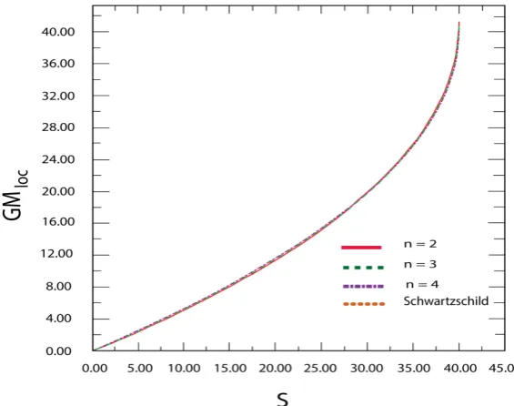
In Figure 8, we plot the Energy as a function of the entropy. It can be seen that, in the local framework, the energy and the temperature T are both positive.

(14)

[image:14.595.230.513.73.296.2]

Figure 8. Graph for GM S n

( )

, _loc for n going from 2 to 4 and Schwarzschild r = 15,

2 5

10

κη ₌ − _and 2

0.4 10 n n

ψ ₌ _× − _.

1

d d d

loc loc loc

loc

loc r H H _r

GM GM T

C

T r r

−         =_ _ = ⋅_ _    

  _ _ (39)

The subscript is there to show that we are calculating this quantity in a fixed po-sition. We work with Equation (39) and give us

(

)

(

)

(

) (

)

2 1 2 2 2 d

1 8π 1

d 2

1 8π 1 8π ,

n loc

n H H

n n

n H n H

GM r

G n r

r

r G r r G r

η ψ

η ψ η ψ −

= − − +   ×_ − − − − − _ (40)

(

) (

)

(

)

(

)

(

) (

)

1 2 2 2 2 2 3 2 2 2 d

1 8π 1 8π

d

1 8π 1

2

1 8π 1 8π

n n

loc

n H n H

H

n H

n H

n n

n H n H

T

v r r G r r G r

r T

r G n r

r G r r G r

η ψ η ψ

η ψ

η ψ η ψ

− + −   = ×_ − − − − − _ + − − +   ×_ − − − − − _ (41)

In Figure 9, we see the local heat capacity plotted for the classical case and the 2

n= to 4 and the local form for the Schwarzschild black hole. It can be ob-served that for the local case, it is possible to obtain an analysis for the thermo-dynamics of black holes for both ψ<0 and ψ>0 to r = 10. It can be seen that the curves for heat capacity are similar for the case n>2. In fact in both cases the r limit of truncates the function.

(15)

[image:15.595.87.538.61.268.2]

Figure 9. Graph for Cloc

(

r nH,

)

for the n=2, n=3 and n=4 and the Schwarzschild for black hole cases, for fixed

10

r= , 2 5

10

κη ₌ − _and 2

0.4 10 n n

ψ ₌ _× −

 .

observed as r grows and the transition to positive values happens even for bigger black hole. This transition is yet to be explained and it occurs even for the clas-sical Schwarzschild case in the local analysis, but not in the most usual global calculation where it remains negative for every value of rH. It can be observed

that for the local case, it is possible to obtain case for ψ >0, that to n>2 has been similar to case ψ <0, in the case of small r.

With Figure 10 it can be seen more easily that the function of the specific heat is stopped precisely at the point rlimit. Now we can analyze the case n=2,

where another phase transition appears where the specific heat changes direction and direction in case ψ >0. It is found that when r is large this would happen for all n. However, when r is very large, the specific heat becomes totally negative and BH will not even form.

Turning to the transition of the entropy phase, due to the correction intro-duced by the

f R

( )

theory discussed in [29], we can have two cases the first for

0

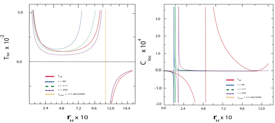
ψ < _{, which is analyzed in a shown in}_{Figure 11}_{on the left to}_n_{= 2. The} Hawking temperature introduces a maximum limit for the horizon radius rH,

which divides a permitted region with, THW >0, of a forbidden region THW <0.

This maximum limit in the radius of the horizon rH can be calculated using the

Equation (26) and corresponds to the solid line of the graph.

An interesting analysis is that the limit of rmax that appears in the

tempera-ture of Hawking is also present in the local case. In the local case, this boundary also divides a permitted region of a forbidden region, and this happens when the position

r

=

r

Hmax. When

r

>

r

Hmax, the minimum temperature decreases, but

the allowed region always has the same size as

r

Hmax.

This behavior can be seen in the graph of Figure 11 on the right, showing the value of

r

Hmax for n = 2, considering different values of r. It can be shown that

(16)

[image:16.595.65.536.64.279.2]

Figure 10. Local heat capacity for n = 2 as a function of the position, 2 5

10

κη ₌ − _and 2

0.4 10 n n

ψ _{= −} _× − _.

Figure 11. Local temperature in the vicinity of rHmax for n = 2 in panel left with

2

0.4 10 n n

ψ _{= −} _× − _{compared with Hawking}

temperature where rHmax=111.8033989 and in panel right the heat capacity.

The existence of a rH limit for black holes that has been studied in the case

0

ψ < repeats to ψ>0 existing a value of r_H that can not be passed

r

H_max.

The Hawking temperature for ψ >0 has no minimum point becoming nega-tive, the

r

Hmax can be found when that temperature is zero by doing the zero

expression (30) that gives us:

(

)

max

1 2 2

1 1

H

n

r

n

κη ψ

 − 

= _ ₊ _

  (42) In the local case we have a behavior similar to ψ <0 the maximum value for

[image:16.595.59.537.309.523.2]

(17)

DOI: 10.4236/jhepgc.2019.53032 603 Journal of High Energy Physics, Gravitation and Cosmology region to the forbidden region, even when

r

<

r

Hmax in the vicinity of rmax. If

we analyze the heat capacity we can observe that the validity limit to r is very small and far from

r

Hmax because the heat capacity became negative and the

black hole is not stable.

3.3. The Thermodynamical Phase Transitions for the Black Hole

Systems

We shall take care in this section of the possible phase transitions of the system we are considering. The first one is the Hawking-Page phase transition. It occurs whenever the function that gives the behavior of the Helmholtz free energy with the radius of the horizon has a root which is a minimum of this function.

(

2

)

(

)

2

1 1

1 1 π 0

2 4 H HP HW HP HP r r n n

n HP HP n HP HP HP

F GM T S

r r r T r

κη ψ ψ

= = −   = _ − − _ − + =

(

)

2 1 π

1 1 1 1 0

2 2 2

H HP

HW

n n

HP

n HP HP n HP HP

H r r

F n

n r T r r

r ₌ κη ψ ψ

∂  ₌ _ ₋ ₋ ₊ _₋  ₊ ₊   ₌

 _∂    _ _ _ _

  (43)

where THP is the Hawking-Page temperature. We find the radius and the

Hawking-Page temperature as given below:

(

)

2 1 1 1 π 1 1 2 n n HP HW HP n HP n HP n r T r n r κη ψ ψ  − − +    =  _{+ +}      _ _    (44)

(

)

1 2 1

1 1 1 2 2 n HP n n n r α ψ  ₋ _{+ ± ∆}    =       (45)

(

)

2

(

) (

)

2 2 2

1 4 1 4 1

n n n n

α

∆ = + − + + + + ₍₄₆₎

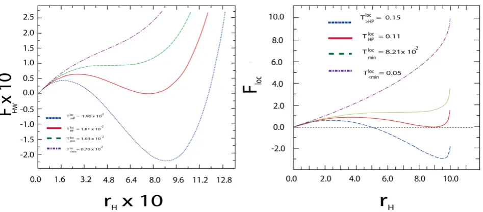
In Figure 12, the free energy question can be analyzed by considering the Hawking-Page phase transition showing its phase change for each value of n us-ing Hawkus-ing’s formalism. In the local case we can have this transition for both

0

ψ < and ψ >0. Repeating what happens in the case of the Hawking-Page ra-dius, these values are very close, so we chose n=2 to do the analysis as shown in Figure 13.

In Figure 13, we present the possible regimes for the free energy in the case 2

n= . The same analysis applies for the others orders of n. The Hawking case that corresponds to ψ <2 0 was plotted in the panel of the left. In this case, we

have a negative cosmological constant. In the right plot, we have ψ >2 0 that

have similar results to ψ <2 0 in the local case, which can represents when

0

ψ > _{the case with a positive cosmological constant.}

(18)

[image:18.595.236.513.65.308.2]

Figure 12. Graph of FHW for the n-order going from 2 to 5, where GM =1,

2 5

0.3 10

κη ₌ _× − _and 2

0.4 10 n n

ψ _{= −} _× − _.

Figure 13. Graph for F for each n = 2, 2 5

0.3 10

κη ₌ _× − _{. The solid line is the Hawking-Page free energy, the dashed line is the}

minimal energy the dashed dotted line is the energy when T>THP and the dotted line is the energy when T<Tmin and in (a)

the Hawking framework 2

0.4 10 n n

ψ _{= −} _× − _{; (b) The local framework} 2

0.4 10 n n

ψ ₌ _× − _.

by the dashed curve, we have a region of pure radiation. The solid curve represents the Hawking-Page temperature that gives us the Hawking-Page Phase transition. The expression, for the minimum of the temperature in Hawking case, can be readily worked out and gives us

(

)

( )

2

1

min 2 min

min

1

1 1

4π

n

T n r

r

κη _ψ −

 

= _ − − + _

[image:18.595.64.538.356.564.2]

(19)

(

)

(

)

1 2 2

min ₂

2

1

r

n

κη

ψ

− − 

 

=

 − 

  (48) As previously discussed, this work considers the boundary of the weak field approximation in a region in the vicinity of the BH with the defect. For this rea-son, we do not contemplate the asymptotic limits. However, whenever n=2 and ψ is negative, the behavior of BH in the f(R)-model considering the Hawking framework resembles the one which occurs in the case of the negative cosmological factor corresponding to the Anti-de-Sitter case. This case is ex-tremely important for the study of the quantum behavior of gravitational sys-tems.

So far, the case analyzed considers ψ <n 0, which can be treated by the

Hawking’s formalism. In the case of the local formalism, it is possible to verify that independently of ψn, it was possible to study both behaviors.

In the graph of Figure 14, the study of the compatibility between the two formalisms can be found. It can be verified that both present the same critical behavior if we choose the value in the local quantities of the fixed point where local quantities are calculated.

In Figure 14, it can be seen that both the case of ψ <n 0 to local and

Hawk-ing cases, can present the same set of minima and HawkHawk-ing-Page temperature, showing compatibility between the two theories. It is always possible to find the same set of values if we regulate the values of r in local formalism. In this Figure, this happens when, for a given Hawking-Page temperature, in local formalism, we set r so that the Hawking-Page temperature value is consistent with Hawk-ing’s formalism.

[image:19.595.236.508.476.687.2]

In Figure 15, a comparison was made between the heat capacity calculated in

Figure 14. Graph for T for each n = 2, 2 5

0.3 10

κη ₌ _× − _and 2

0.4 10 n n

ψ _{= −} _× − _with_r₌

(20)

[image:20.595.209.540.64.284.2]

Figure 15. Graph for the comparation between Cloc and CH for each n = 2,

2 5

0.3 10

κη ₌ _× − _and 2

0.4 10 n n

ψ _{= −} _× − _with 2

1.3408 10

HP

T = × − for both cases.

Hawking’s formalism (CHW) and Local (Cloc) in the case of psi < 0. In the figure

to the left it can be seen that in the case of Hawking formalism, as indicated in the graph, there are three distinct regions, the first comprises a negative CHW

for *

H

r

<

r

. The other region corresponds to a positive CHW for

* c

H

r

<

r

<

r

and the latter comprises the region given by c

H

r

>

r

. In the figure to the right, upper part, this behavior was further detailed. Analyzing the graph to the right, it can be clearly seen that _r* coincides with the forbidden/allowed transition

region. The region * H

r

<

r

is a forbidden layer because it has specific heat neg-ative. The region * c

H

r

<

r

<

r

is permissive where we find a stable black hole. In this region the temperature starts from the minimum and grows with the ra-dius of the horizon while the heat capacity decreases. In this region the black hole is stable. When c

H

r

>

r

we have again a forbidden region.

The other curve of the specific heat of Figure 15 left corresponds to the local case. For the comparison the parameters of the local model were adjusted to

105.57

r= . With these conditions, the Hawking-Page temperature can be ob-tained. In Figure 15 the right panel down can analyze the detail of the local case. It can be seen that in this case the solution to the black hole presents two possi-bilities corresponding to both heat capacity and temperature greater than zero. It can be seen that there is a region between *

min H

r

<

r

<

r

, where a black hole so-lution is possible, but this is unstable because the temperature decreases with the radius of the horizon going to a more stable location that is rmin. This region is

called a small black hole. The other region presents, as in the case of the Hawk-ing formalism, the temperature increasHawk-ing with the increase of rh, showing that

for the increase of the black hole this is giving more energy, for that reason warmer. This region is called the Great Black Hole.

(21)

[image:21.595.212.537.66.282.2]

Figure 16. Graph for the comparation between Cloc for ψ <n 0 and Cloc for ψ >n 0

each n = 2, κη2=_{0.3 10}× −5 and 2

0.4 10 n n

ψ ₌_ _× − _r_{= 10 and}

0.1078

HP

T = .

with ψ <0 and ψ >0 for the same Hawking-Page temperature was analyzed. As in the case of Figure 15, where the ψ <0 case was analyzed, it can be seen that the limits for large rH depend on the value of r. Comparing these two cases,

it can be analyzed that when ψ >0, has only one allowed region for

r

*

<

r

_H

<

r

c, where we have both temperature and calorific capacity positive. In this region there may be several possibilities, the temperature decreases as the heat capacity decreases, for increasing rH, small black hole. A region where temperature

in-creases and specific heat dein-creases and a region where both specific heat and temperature increase with increasing horizon radius rH this region is the big

black hole.

4. Closing Remarks

In this work, the solution of a black hole in a region containing a global mono-pole in a class of f(R) gravity models has been investigated using a power law approach. To pursue our investigation, we have considered the weak field ap-proximation for small radial coordinate values, assuming the validity of the con-dition of the Equation (22). In this his region, it is possible to analyze the beha-vior of BH solutions for n>0 and ψ_n positive and negative.

The very goal of this work is the analysis of the thermodynamical behavior of the black hole, considering two possible formalisms: Hawking’s, on the one hand, and local formulation on the other hand.

In the case of Hawking’s approach, it was possible to study the case where

0

n

ψ < as being stable, by studying the positivity of the temperature with the positivity of the heat capacity. This black hole was called a large black hole, lo-cated for the radius of the horizon, rH >rmin. For rH <rmin, we have an

unsta-ble black hole despite having a region between *

min

H H

(22)

DOI: 10.4236/jhepgc.2019.53032 608 Journal of High Energy Physics, Gravitation and Cosmology capacity is positive and the temperature is positive.

The case with ψ >n 0 has been tackled in the local formalism; this

frame-work is actually valid for both ψn positive and negative. The local case was

stu-died in more details for ψ >n 0 and a BH with similar characteristics as in the

Hawking’s treatment was obtained, if we work in the region of validity. In this work, we also compared these two regimes, by analyzing not only the relation-ship between heat capacity and temperature, but also the phase transitions that the system may undergo. It has been found that, for small values of rH, the two

formalisms are compatible. When rH grows, it reaches a value where the BH

undergoes another transition, now related to a change of behavior in the heat capacity. In the case of the thermodynamics with the Hawking formalism, the heat capacity passes from a region where it decreases with increasing tempera-ture to a region where it increases with temperatempera-ture. In the local case the heat capacity for

r

_H

>

r

_min always decreases with temperature going to negative values.

Based on the assumption that heat capacity and temperature are not sufficient to guarantee stability, the Hawking-Page phase transition, which applies to both Hawking’s formalism and local formalism, was also considered. It has been checked that, in both formalisms, a Hawking-Page phase transition exists as anoth-er attribute in favor of the stability of BH.

The case with n=2 has also been contemplated. The relevance of this case lies in the fact that the power law parameter,

ψ

2, can act as a cosmological

con-stant, that can be positive or negative in this region.

The idea now is to inspect the asymptotic region that occurs for the case < 0

n . With this analysis, it will be possible to study the limits of-Sitter and An-ti-de Sitter and the behavior on the borders. Besides the asymptotic behaviors, it is also interesting to study the potential generators of the power law presage that can be clarified when discussing the problem all over the space. In future works, we intend to investigate this case, that might be important for the AdS/CFT context for the n=2 situation. These aspects are under study and shall be the subject of a forthcoming work. It is possible to solve the stability problem for a negative ψ2 and to use the same thermodynamical procedure that we have

used here. The importance, in the AdS context, is the fact that this black hole presents an angular deficit, and it is important to study the holographic principle of this object. We have shown in [34] that the structure of the angular deficit in a theory in

D

= +

(

1 3

)

is preserved on the

(

1 2

+

)

boundary and, in our case, the defect is preserved in

D

= +

(

1 2

)

. The AdS4/CFT3 is very important in studying planar materials like graphene and topological insulators. The intro-duction of the defect in this type of systems gives us current properties in these materials and it may become a relevant aspect of our work, opening up new ap-plication possibilities for our model. Another issue that we can pick up to study is the behavior of the objects near these systems [35] with both regimes for ψ2.

(23)

criti-DOI: 10.4236/jhepgc.2019.53032 609 Journal of High Energy Physics, Gravitation and Cosmology cal temperature [36].

Acknowledgements

F. B. Lustosa would like to thank CNPq-Brasil for his MSc Fellowship at the In-stituto de Fsica of Universidade Federal Fluminense. The authors express their gratitude to T.R.P. Caramês for clarifying discussions.

Conflicts of Interest

The authors declare no conflicts of interest regarding the publication of this pa-per.

References

[1] Buchdahl, H.A. (1970) Non-Linear Lagrangians and Cosmological Theory. Monthly Notices of the Royal Astronomical Society, 150, 1-8.

https://doi.org/10.1093/mnras/150.1.1

[2] Morais, J., Bouhmadi-Lpez, M. and Capozziello, S. (2015) Can f(R) Gravity Contri-bute to (Dark) Radiation? JCAP, 1509, 041.

[3] Takahashi, K. and Yokoyama, J. (2015) Equation of State of Dark Energy in f(R) Gravity. Physical Review D, 91, Article ID: 084060.

[4] Nojiri, S. and Odintsov, S.D. (2011) Unified Cosmic History in Modified Gravity: From F(R) Theory to Lorentz Non-Invariant Models. Physics Reports, 505, 59-144. https://doi.org/10.1016/j.physrep.2011.04.001

[5] Sotiriou, T.P. and Faraoni, V. (2010) f(R) Theories of Gravity. Reviews of Modern Physics, 82, 451.https://doi.org/10.1103/RevModPhys.82.451

[6] Perlmutter,S., et al. (1999) Measurements of Ω and Λ from 42 High-Redshift Su-pernovae. The Astrophysical Journal, 517, 565-586.https://doi.org/10.1086/307221 [7] Hu, W. and Sawicki, I. (2007) Models of f(R) Cosmic Acceleration That Evade Solar

System Tests. Physical Review D, 76, Article ID: 064004. https://doi.org/10.1103/PhysRevD.76.064004

[8] Appleby, S.A. and Battye, R.A. (2007) Do Consistent F(R) Models Mimic General Relativity plus Lambda? Physics Letters B, 654, 7-12.

[9] Starobinsky, A.A. (2007) Disappearing Cosmological Constant in f(R) Gravity.

JETP Letters, 86, 157-163.https://doi.org/10.1134/S0021364007150027

[10] Ohta, N., Percacci, R. and Vacca, G.P. (2015) Flow Equation for f(R) Gravity and Some of Its Exact Solutions. Physical Review D, 92, Article ID: 061501.

[11] Corda, C. (2009) Interferometric Detection of Gravitational Waves: The Definitive Test for General Relativity. International Journal of Modern Physics D, 18, 2275-2282.https://doi.org/10.1142/S0218271809015904

[12] Bekenstein, J.D. (1972) Black Holes and the Second Law. Lettere al Nuovo Cimento, 4, 737-740.https://doi.org/10.1007/BF02757029

[13] Bekenstein, J.D. (1973) Black Holes and Entropy. Physical Review D, 7, 2333. https://doi.org/10.1103/PhysRevD.7.2333

[14] Bekenstein, J.D. (1974) Generalized Second Law of Thermodynamics in Black-Hole Physics. Physical Review D, 9, 3292.https://doi.org/10.1103/PhysRevD.9.3292 [15] Hawking, S.W. (1975) Particle Creation by Black Holes. Communications in

(24)

[16] Cai, R.-G., Cao, L.-M. and Ohta, N. (2010) Black Holes in Gravity with Conformal Anomaly and Logarithmic Term in Black Hole Entropy. JHEP, 1004, 082.

[17] Myung, Y.S., Kim, Y.-W. and Park, Y.-J. (2008) Thermodynamics and Phase Tran-sitions in the Born-Infeld-Anti-De Sitter Black Holes. Physical Review D, 78, Article ID: 084002.

[18] Biswas, R. and Chakraborty, S. (2011) Geometry of the Thermodynamics of the Black Holes in Hořava-Lifshitz Gravity. General Relativity and Gravitation, 43, 41-50.https://doi.org/10.1007/s10714-010-1067-4

[19] de la Cruz-Dombriz, A., Dobado, A. and Maroto, A.L. (2009) Black Holes in f(R) Theories. Physical Review D, 80, Article ID: 124011.

[20] Kibble, T.W.B. (1976) Topology of Cosmic Domains and Strings. Journal of Physics A, 9, 1387.https://doi.org/10.1088/0305-4470/9/8/029

[21] Vilenkin, A. (1985) Cosmic Strings and Domain Walls. Physics Reports, 121, 263-315.https://doi.org/10.1016/0370-1573(85)90033-X

[22] Barriola, M. and Vilenkin, A. (1989) Gravitational Field of a Global Monopole.

Physical Review Letters, 63, 341.https://doi.org/10.1103/PhysRevLett.63.341 [23] Caramês, T.R.P., Bezerra de Mello, E.R. and Guimarães, M.E.X. (2011)

Gravitation-al Field of a GlobGravitation-al Monopole in a Modified Gravity. International Journal of Mod-ern Physics: Conference Series, 3, 446.

[24] Marunovic, A. and Murkovic, M. (2014) A Novel Black Hole Mimicker: A Boson Star and a Global Monopole Nonminimally Coupled to Gravity. Classical and Quantum Gravity, 31, Article ID: 045010.

[25] Multamaki, T. and Vilja, I. (2006) Spherically Symmetric Solutions of Modified Field Equations in f(R) Theories of Gravity. Physical Review D, 74, Article ID: 064022.https://doi.org/10.1103/PhysRevD.74.064022

[26] Caramês, T.R.P., Bezerra de Mello, E.R. and Guimarães, M.E.X. (2012) On the Mo-tion of a Test Particle around a Global Monopole in a Modified Gravity. Modern Physics Letters A, 27, Article ID: 1250177.

https://doi.org/10.1142/S0217732312501775

[27] Yu, H.-W. (1994) Black Hole Thermodynamics and Global Monopoles. Nuclear Physics B, 430, 427-440.https://doi.org/10.1016/0550-3213(94)00339-4

[28] Man, J. and Cheng, H. (2013) Thermodynamic Quantities of a Black Hole with an f(R) Global Monopole. Physical Review D, 87, Article ID: 044002.

https://doi.org/10.1103/PhysRevD.87.044002

[29] Faraoni, V. (2010) Black Hole Entropy in Scalar-Tensor and ƒ(R) Gravity: An Overview. Entropy, 12, 1246-1263.https://doi.org/10.3390/e12051246

[30] Bardeen, J.M., Carter, B. and Hawking, S.W. (1973) The Four Laws of Black Hole Mechanics. Communications in Mathematical Physics, 31, 161-170.

[31] Hawking, S.W. (1974) Black Hole Explosions? Nature, 248, 30-31. https://doi.org/10.1038/248030a0

[32] Tolman, R.C. (1930) On the Weight of Heat and Thermal Equilibrium in General Relativity. Physical Review, 35, 904.https://doi.org/10.1103/PhysRev.35.904

[33] Davies, P.C.W. (1978) Thermodynamics of Black Holes. Reports on Progress in Physics, 41, 1313-1355.https://doi.org/10.1088/0034-4885/41/8/004

(25)

[35] Ballon-Bayona, A., Ferreira, C.N. and Otoya, V.J.V. (2013) DBI Equations and Ho-lographic DC Conductivity. Physical Review D, 87, Article ID: 106007.

https://doi.org/10.1103/PhysRevD.87.106007