Full Terms & Conditions of access and use can be found at
http://www.tandfonline.com/action/journalInformation?journalCode=raag21
Download by: [University of St Andrews] Date: 29 November 2017, At: 04:31
ISSN: 2469-4452 (Print) 2469-4460 (Online) Journal homepage: http://www.tandfonline.com/loi/raag21
Revisiting the Past: Replicating Fifty-Year-Old Flow
Analysis Using Contemporary Taxi Flow Data
Urška Demšar, Jonathan Reades, Ed Manley & Michael Batty
To cite this article: Urška Demšar, Jonathan Reades, Ed Manley & Michael Batty (2017):
Revisiting the Past: Replicating Fifty-Year-Old Flow Analysis Using Contemporary Taxi Flow Data, Annals of the American Association of Geographers, DOI: 10.1080/24694452.2017.1374164
To link to this article: https://doi.org/10.1080/24694452.2017.1374164
© 2018 The Author(s). Published with license by Taylor & Francis© Urška Demšar, Jonathan Reades, Ed Manley, and Michael Batty
View supplementary material
Published online: 27 Nov 2017.
Submit your article to this journal
Article views: 42
View related articles
Revisiting the Past: Replicating Fifty-Year-Old Flow
Analysis Using Contemporary Taxi Flow Data
Urska Demsar ,* Jonathan Reades ,yEd Manley ,zand Michael Batty z
*School of Geography & Sustainable Development, University of St. Andrews
yDepartment of Geography, King’s College London
zCentre for Advanced Spatial Analysis, University College London
Over sixty years ago, geography began its so-called quantitative revolution, where for the first time statistical methods were used to explain the spatial nature of geographic phenomena. Computers made some of this possi-ble, but their limited power did not allow for more than relatively small analytic explorations and consequently many of these earlier ideas are now buried in the mists of time. Here we attempt to replicate one of these early analyses using taxi flow data collected in 1962 and originally used by Goddard (1970; then at the London School of Economics) to extract functional regions within London’s city center. Our experiment attempts to replicate Goddard’s methodology on a modern taxi flow data set, acquired through Global Positioning System tracking. We initially expected that our analysis would be directly comparable with Goddard’s, potentially pro-viding insights into temporal change in the spatial structure of the city core. Attempts at replicating the origi-nal aorigi-nalysis have proved enormously difficult, however, for several reasons, including the many subjective choices made by the researcher in articulating and using the original method and the specific characteristics of contemporary taxi flow data. We therefore opt to replicate Goddard’s approach as closely and as logically as possible and to fill in gaps based on statistically informed choices. We have also run the analysis on two spatial scales—Central London and a wider area—to explore how scales of analyses that were beyond the capacities of Goddard’s early computations also help to shape our understanding of the results he obtained.Key Words: comparative spatial analysis, movement analytics, principal component analysis (PCA), quantitative method develop-ment, replication.
六十多年前,地理学展开了所谓的计量革命,其中统计方法首度被用来解释地理现象的社会本质。计算
机让此一方法部分成为可能,但其有限的力量,却仅能考量相对小型的分析探讨,因而导致诸多早期的想
法,被深埋在时间之中。我们于此运用在1962年搜集、并且原本由哥达德(1970年,接着是在伦敦政经
学院)用来取得伦敦市中心功能区域的出租车流数据,尝试复製此般早期的分析。我们的实验,企图透过
全球定位系统追踪,在当代出租车流数据集中复製哥达尔的方法。我们原本期待自身的分析能够直接与
哥达尔的研究进行比较,并对于城市中心空间结构的时间变迁提出洞见。但复製原本分析的尝试,却因
诸多原因,证实是相当困难的,包括研究者在表达与使用原初方法时做出的诸多主观选择,以及当代出租
车流数据的特徵。我们因此选择最接近和最具逻辑的方法来复製哥达尔的方法,并根据统计所告知的选
择来填补阙如。我们同时在两个空间尺度上进行分析——伦敦市中心与较广泛的区域——探讨超出哥
达尔早期计量能力的分析尺度, 如何有助于形塑我们对他所得到的研究结果之认识。 关键词: 比较空
间分析,移动分析,主成分分析(PCA),计量方法发展,复製。
Hace mas de sesenta anos que la geograf~ ıa empezo la llamada revolucion cuantitativa, mediante la cual por pri-mera vez se usaron metodos estadısticos para explicar la naturaleza espacial de los fenomenos geograficos. Los computadores hicieron posible algo de esto, aunque su limitado poder solo permitio exploraciones analıticas rel-ativamente peque~nas y consecuentemente muchas de estas ideas tempraneras se hallan ahora sepultadas en las nieblas del tiempo. Aquı intentamos replicar uno de aquellos analisis usando datos del flujo de taxis recolecta-dos en 1962, utilizarecolecta-dos originalmente por Goddard (1970; entonces en la London School of Economics) para extraer regiones funcionales dentro del centro urbano de Londres. Nuestro experimento intenta replicar la metodologıa de Goddard a partir de un conjunto moderno de datos de flujo de taxis, adquirido por medio de ras-treo del Sistema de Posicionamiento Global. Inicialmente esperabamos que nuestro analisis serıa directamente comparable con el de Goddard, generando potencialmente perspectivas del cambio temporal en la estructura espacial del nucleo de la ciudad. Sin embargo, los intentos por replicar el analisis original han resultado
Ó2018 Urska Demsar, Jonathan Reades, Ed Manley, and Michael Batty. Published with license by Taylor & Francis.
This is an Open Access article distributed under the terms of the Creative Commons Attribution License (http://creativecommons.org/licenses/by/4.0/), which permits unrestricted use, distribution, and reproduction in any medium, provided the original work is properly cited.
Annals of the American Association of Geographers, 0(0) 2017, pp. 1–18 Initial submission, May 2017; revised submission, July 2017; final acceptance, July 2017
enormemente difıciles por varias razones, incluyendo las numerosas decisiones subjetivas del investigador para articular y usar el metodo original, y las caracterısticas especıficas de los datos contemporaneos sobre flujo de taxis. En consecuencia, optamos por replicar el enfoque de Goddard tan cerca y tan logicamente como fuese posible, llenando los vacıos con base en selecciones estadısticamente respaldadas. Tambien hemos corrido el analisis a dos escalas espaciales ––el centro de London y unarea mas amplia–– para explorar el modo como las escalas de los analisis que estuvieron fuera de las capacidades de los calculos de Goddard tambien ayudan a con-figurar nuestra comprension de los resultados obtenidos.Palabras clave: analisis espacial comparativo, analıticas del movimiento, analisis de componentes principales (PCA), desarrollo del m etodo cuantitativo, replica.
S
ixty years ago, geographers first began to explore spatial patterns using rudimentary statistical methods that sought to extract the key determi-nants of spatial structure at a range of scales from a multitude of independent variables (Berry 1964, 1970). Regression, correlation, principal components, and factor analysis represented the cutting edge of quantitative geography. In 1970, Goddard published an article detecting functional regions in a set of inter-actions (taxi traffic flows) between small partitions (zones) in a very large city center. Goddard (1970) collected and coded movement data from taxi drivers’ log books produced as part of the London Traffic Sur-vey in 1962, from which he was able to generate an origin–destination flow matrix describing properties of taxi movement in London. He then applied a combi-nation of statistical and data mining techniques to extract overlapping functional regions shaped by trips to and from important locations (e.g., mainline rail stations) distributed around London’s central core.Goddard was not the only person at this time using transportation and communication flow data to derive regions rooted in functional interactions. This was, in fact, quite a popular approach to the analysis of urban structure (e.g., Berry 1964; Illeris and Pedersen 1968; Davies 1979), bolstered by the emergence of spatial interaction modeling (Voorhees 2013). However, the basic question of how best to partition a city into coherent regions based on the movement patterns through the urban space remains germane. Indeed, our increased mobility and ability to interact at a distance makes the data-driven interrogation and derivation of regional structure more important than ever. Flow data, however, have changed a great deal since the 1960s, becoming much more extensive through the development of sensors and systems able to capture data in real time and complementing or even sup-planting the manual surveys that were the dominant mode of collection in the past. Reflecting the preoccu-pations of our “network society” (Castells 1996), methods derived from social network analysis are par-ticularly popular (Demsar,Spatenkova, and Virrantaus
2007; Ratti et al. 2010; Expert et al. 2011). O’Sullivan and Manson (2015) also noted a rapid increase in physicists working on geographical topics, including flows and interactions—articulating and “solving the city” in these terms (Bettencourt and West 2010).
In this article, we explore the potential relevance of one of these early flow-based regionalization methods to modern flow data and contemporary problems. Through replication, we hope to revitalize and reex-amine a regionalization methodology rooted in a com-bination of principal component analysis (PCA) and hierarchical clustering to derive a set of internally coherent regions based on the patterns of taxi flows. We do so using modern Global Positioning System (GPS) taxi tracking data that we expected would pro-vide an opportunity to investigate how the functional structure of taxi movement in London has changed in the last fifty years. In seeking to replicate Goddard’s work, though, we discover that a straightforward step-by-step replication is impossible; instead, we are forced to “reinvent” certain steps to obtain interpretable and useful results. Nonetheless, although we uncover some long-overlooked issues in the original work, we also find that this approach offers specific analytical advan-tages over more recent—and trendy—regionalization methods borrowed from network science and social network analysis (for an overview, see Farmer and Fotheringham 2011), an issue to which we return in the Conclusion.
The remainder of this article is structured as follows. First we set the context by reviewing the literature on PCA, flow-based regionalization methods, and application of PCA to flow data. Then we introduce the taxi data used by Goddard and those that we have worked with. In the Methodology section, we set out Goddard’s methodology step by step and in parallel describe changes that were required to adapt it, together with a logical reasoning that led us to each specific change. This is followed by the results of the two spatial scales of analysis, first for central London (to follow the geographic extent of Goddard’s study) and an extension to the wider city. We conclude with
a discussion of how revisiting seminal works such as this can bring new insights to contemporary research and lead to new knowledge derived from modern flow data.
Related Work
Understanding PCA
Since its development at the beginning of the twen-tieth century, PCA has been used in a range of scien-tific disciplines, including geography (Demsar et al. 2013) for dimensionality reduction, orthogonalization, and the exploration of data cloud structures. A full mathematical description of PCA can be found in Jol-liffee (2002), whereas here we briefly review the aspects of the method that are relevant to the analysis and interpretation of our and Goddard’s results.
PCA defines a linear mapping between then varia-bles defining some original data space and a new, orthogonal coordinate system that is aligned with the directions of greatest variance in the data. Imagine freely rotating the axes within a cloud of data points so that the first axis aligns with the widest part of the cloud, the second axis with the next widest part, and so on. Each axis is orthogonal (i.e., at right angles) to all the others and hence they are linearly independent from one another and can be treated as independent variables for descriptive and analytical purposes. These new axes are known as principal components (PCs).
For data analysis, PCs are typically derived from the correlation or covariance matrices rather than from the direct data matrix. In the covariance matrix, the vari-ance on each variable is taken without standardization, whereas in the correlation matrix all variables are stan-dardized to the same scale. If the variables have very different scales (e.g., one is measured in centimeters per year and another in kilometers per hour) then the covariance matrix will be strongly biased by the abso-lute numerical value of the smaller scale. The selected matrix (covariance or correlation) is then processed via eigendecomposition to yield a set of eigenvector and eigenvalue pairs. In Goddard’s and our cases, the PCA decomposition is applied on a correlation matrix.
The eigenvectors define the transformations (e.g., scaling and rotation) needed to move between the original and new coordinate systems, whereas the eigenvalues give the scaling factor of the transforma-tion. Consequently, the direction of each eigenvector corresponds to one PC, and the amount of variance
explained by the PC can be derived from the magni-tude of the respective eigenvalue. When sorted according to their eigenvalues, the first PC is oriented in the direction of the greatest variance in the data cloud, the second PC in the direction of the next greatest amount of variance, and so on.
In anm£ndata matrix, the new space defined by the eigenvectors can have at most min(m,n) dimen-sions; that is, the space is bound by the minimum of the columns or the rows of the matrix. In spatial applica-tions, it is usually the case thatn<<m(i.e., there are many more observations in space than there are attrib-utes at each location), and so normally there are at mostnPCs derived from the original data. Much of the information contained in the original data, however, can often be reconstructed from an even smaller set (k, wherek<<n) of eigenvectors: those with theklargest eigenvalues. PCA is therefore often used for dimension-ality reduction, where the selection of an appropriatek depends on the individual data set; heuristics exist for this purpose, and some, such as the scree plot (Berthold and Hand 2007), are graphical, whereas others, such as the contributed variance (Jolliffee 2002), are prag-matic. Our analysis employs both types of heuristics, as further described in the Methodology section.
The Use of Flow Data for Regional Analysis
The use of transportation and communications flow data to derive regions rooted in functional interactions can be traced back to the rise of transportation plan-ning in the 1950s (Voorhees 2013) and the increased accessibility of computers able to perform matrix anal-yses at speed (Berry 1964). Although today’s desktop and server systems might make some of the analytical challenges faced by these earlier researchers seem almost quaint, the basic question of how best to parti-tion a set of zones into analytically useful regions remains a major preoccupation of urban geography and spatial analysis (Roth et al. 2011; Reades and Smith 2014).
Although it is well understood that different region-alization methods can produce substantially different optimal sets of smaller regions, there are two areas that merit particular attention. First, it is easy to forget that there exist many possible realizations of that partition-ing, depending on which attributes are given weight and why; second, it is rarely noted that many parti-tioning methods exclusively assign each zone to a sin-gle region based on some concept of containment or
integration. Given that we can easily select arbitrary temporal or spatial slices from the data set, the manner in which we process, clean, and select data for the analysis will have a significant effect on the regions identified: Weekday data might better capture regions rooted in workplace interactions, whereas weekend data might be better for understanding social or recrea-tional connections.
The second issue is more subtle because the exclu-sive association between zones (nodes) and regions (groups of nodes) can be a natural, and indeed power-ful, approach to understanding human geography (Ratti et al. 2010; Expert et al. 2011). Where, for instance, though, there is evidence of polycentricism and of multiple business centers generating and receiving large numbers of trips across a wide area (Taylor, Evans, and Pain 2006), it is worth asking whether this type of exclusive partitioning is appro-priate. A study undertaken by Zhong et al. (2014), although appropriate for exclusive regional defini-tions, is not appropriate for improving our ability to see overlapping flows where one zone contributes to multiple regions simultaneously. Additional issues arise with constraints governing permissible regions; for instance, intramax modeling of commuting flows not only makes exclusive assignments of zones to regions but also requires that the region be consti-tuted from a set of contiguous zones (Nielsen and Hovgesen 2008). Indeed, Goddard (1970) experi-mented with the impact of contiguity constraints as part of his own analysis.
Flow Analysis Using PCA
PCA for spatial analysis became particularly popular in the 1960s and 1970s, as it was one of the first tools available to examine structure in large data sets since, in 1970, spatial interaction data sets were bigger than anything seen thus far. Typically, PCA was employed as a preprocessing orthogonalization method to enable subsequent clustering or cross-classification for group-ing areas into regions on the basis of interzonal similar-ity (Berry 1964). Although less common, a number of studies also attempted to use it on flow data in transpor-tation (Black 1973), telecommunications (Goddard 1973), and, as in this application, taxi journeys (God-dard 1970). Many further uses for PCA have since been found in a geographical context (see Demsar et al. [2013] for an extensive review), but they are not rele-vant for our replication experiment.
Data
The Changing Nature of Geographical Data
The data in Goddard’s (1970) paper were drawn from log books completed by a 10 percent sample of London’s Black Cab taxi drivers during a week in July 1962 as part of the London Travel Survey (LTS). The log book data included journeys made while cruising for fares, as well as the usual fare-paying trips, and were then manually coded to one of sixty-nine traffic analysis zones (TAZs) created by the Office of Popula-tion, Census and Surveys from the 1961 Census. The exact number of journeys undertaken by taxis that year is not known, but we estimate from Goddard’s diagrams that the daily weekday average is on the order of 18,000 trips. The sample would have been manually tabulated into an origin–destination (O/D) matrix suitable for encoding on punch cards as part of a scheduled run—with a turnaround time of twenty-four hours—on the university mainframe. The direct scaling of tabulation effort and physical storage media with data volumes placed tight constraints on the scale of analysis that were then feasible.
In contrast, the modern taxi data set, made avail-able through a partnership with the minicab firm Addison Lee (hereafter called AddLee), was accessed over a high-speed digital network. There are key differ-ences, of course, in the business models used by Black Cabs and AddLee. In fact, back in 1962 when the Black Cab data were assembled, the term business model was unknown and these taxis operated very largely from hailing on the street or by customers going to known taxi ranks. AddLee, however, is bookable and thus skewed toward business accounts (dominated by the movements from high-profile wealthy home and work locations like the City of London). The AddLee data set contains some 1.3 million passenger journeys made between 1 December 2010 and 28 Feb-ruary 2011 using any of the firm’s 2,500 vehicles; it is both complete and spatially extensive, covering all of Greater London and not just the central core.
From AddLee we get a similar weekday average of 19,000 journeys, but we now have access to all of the data, not just a sample, although we should note that there are other taxi firms for which we have not been able to access data. Exact origin and destination were available both via the computer-ized fleet management system and each vehicle’s GPS logs. Because the precision of GPS data theo-retically enables us to identify address-level origins
and destinations, the data were spatially aggregated to minimize the risk of reidentification (Zheleva and Getoor 2007). The aggregation was made to the TAZs currently used by Transport for London that we will define as n origins i D 1, 2, . . ., n and m destinations j D 1, 2, . . ., m. This generates a trip matrix [Tij], which constitutes the basic data for the comparison. Figure 1 shows the relevant histori-cal and contemporary TAZ boundaries, emphasizing the overall stability of these units.
Based on the stability of the spatial units, we expected to be able to replicate Goddard’s procedure in the area of Central London to the point of obtaining comparable results, while also extending the analysis to the entire metropolitan region. In the interests of focusing on functional urban regions (Hall 2009) embodied in work-day travel, we selected only journeys that began after 7 a.m. and finished before 8 p.m. Figure 2 provides an overview of the AddLee data at our two analytical scales. Figure 2A shows the same Central London geography analyzed by Goddard in 1970, and Figure 2B shows a larger inner London set of zones capturing wider flows.
Method
Following Goddard’s paper, our analysis consisted of four steps:
1. Applying PCA to London taxi flows. 2. Dimensionality reduction and rotation.
3. Definition of overlapping functional regions from PC loadings and scores.
4. Definition of nonoverlapping regions based on scores’ similarity.
In this section, we discuss each of these four steps and describe how we replicated them using our modern data.
Step 1: Replicating the Analysis: Applying PCA to London Taxi Flows
As described previously, the data for this analysis consist of an O/D trip matrix [Tij] of AddLee vehicle flows between TAZs in London. Each element Tij of this matrix, also known as a flow matrix, gives us a count of taxi trips starting at origin TAZiand ending at destination TAZj. The diagonal elements represent intrazone flows. Goddard’s original matrix covered cen-tral London and was relatively small (69£69), whereas the AddLee data permits us to define both a comparable
region—consisting of the 133£133 matrix [TC ij] that most closely resembles Goddard’s own study area— and a wider regionRIspanning Central and inner Lon-don with a matrix [TI
ij] that is 391£391 in size. Note that there is, of course, no reason why the analysis could not be applied to the entire data set, a matrix of 1,168 zones that is seventy-seven times larger than Goddard’s and includes a major addition to the main-line station—the international airport—but this takes us further away from any kind of comparative study. Moreover it is only possible now with contemporary computing technologies and was simply impossible when Goddard undertook his analysis.
The trip matrices are viewed as a spatial data set, such that origins can be considered observations and destina-tions are treated as variables. This approach can be thought of as a destination-based analysis, but the trip matrix could be transposed to create a dual problem that treats destinations as observations and origins as variables. This duality is beyond the scope of this analysis; however, we note that this would provide a different picture of the city’s functional regions. Although there has been little explicit consideration of the empirical implications of these primal and dual problems for flow analysis, they are well used in multivariate analysis and are referred to as R-mode and Q-R-mode PCA (Tanaka and Zhang 1999). This issue can also be linked to developments in spatial interac-tion and network theory where the primal and dual prob-lems have been more directly considered (Batty 2013).
The first step in the procedure is to calculate the correlation matrixCijfrom the flow matrixTij. PCA is then applied to the correlation matrixCijto generate a new set of ordered dimensions, the PCs, with the importance of each connected to the amount of varia-tion in the raw data that it explains, which is con-tained in the order of eigenvalues of the PCA decomposition. Goddard then used the eigenvalues for dimensionality reduction, which is where our replica-tion attempt hit the first mathematical obstacle.
Step 2: Challenges for Replication: Dimensionality Reduction and Rotation
Having extracted the PCs, Goddard reported adjust-ing the PCs usadjust-ing varimax rotation. Varimax rotation (Kaiser 1958) was developed for factor analysis (FA) to maximize the variance explained by derived factors while also ensuring that, as far as possible, each one is correlated with only one of the original variables. A similar rotation of PCs is sometimes employed in
atmospheric science (Jolliffe 2002), but its validity is debatable because PCs derived via the correlation or covariance matrices already maximize variance, whereas factors do not necessarily achieve that (see the further discussion later). Hence, not only does rotation of the axes in the PC space risk changing the ordering associ-ated with eigenvalues (Daultrey 1976), but the criterion
of each rotated PC to be as closely bound as possible to a single initial variable is not very meaningful (Harris 2001; Demsar et al. 2013). The use of the varimax rota-tion therefore raises the quesrota-tion of which method Goddard employed: PCA or FA.
[image:7.594.124.464.59.589.2]Goddard reported drawing inspiration for his analy-sis from Rummel’s (1967) classic monograph Figure 1. 1970 and 2011 traffic analysis zones comparison. (A) 1970 zones from 1962 London Traffic Survey; (B) 2011 zones from London Traffic Model.
Understanding Factor Analysis, and the full title of his 1970 publication is “Functional Regions within the City Centre: A Study by Factor Analysis of Taxi Flows in Central London”; however, the article itself dis-cusses only the use of PCA. This confusion matters because, although FA and PCA are related techniques designed to extract meaning from the structure of a
[image:8.594.132.474.64.595.2]data cloud, there are important differences between them. Principal among these is that FA a priori defines how many new dimensions (factors) there should be and fits a model to this number, whereas PCA makes no such assumptions. Therefore, FA could be consid-ered as a data modeling approach for a preexisting hypothesis about the number of latent factors, whereas Figure 2. Flows, origin, and destination volumes. (A) Undirected volumes of AddLee trips between TAZs for Central London; (B) undi-rected volumes of AddLee trips between TAZs for inner and Central London. TAZDtraffic analysis zone. (Color figure available online.)
PCA is a data exploratory technique. See Jolliffe (2002, chapter 7) for a further detailed comparison of PCA and FA.
A further important implication of this difference is that there exists only one solution for PCs, as these describe the data cloud in the best possible way such that the explained variance for each axis is maximized, whereas the model-fitting approach of FA means that, rather than identifying a unique solution where the variance of the new dimensions is maximized, a different model is derived for each different set of factors. Conse-quently, as dimensionality reduction approaches, PCA and FA yield quite different outcomes: In FA we specify the level of reduction because we specify the number of dimensions and the data are mapped onto these, whereas in PCA we select some subset of the extracted dimen-sions that capture the desired share of the variance and discard the rest. This latter is the procedure that Goddard described in his paper, which implies that it was indeed the PCA that was employed and not FA.
Fifty years on there is no way to resolve this confu-sion: At the time, both PCA and FA on a data set of this size employed a standard package stored on a set of punch cards to which the data were then attached on another set of cards. Goddard did not write the program and was advised by the programming advisory service based at Imperial College. Goddard was based at the London School of Economics, but that college had no mainframe on which multivariate software of the kind required could be run (J. Goddard, personal communi-cation August 2011). As users of such systems had little control over the program itself, it is not possible to determine what variant of PCA or FA was used, as all of this information is now lost in the mists of time. God-dard is not able to remember the variant that was used. Because neither the original data nor the original code remain—and the latter would not be machine readable if it did—we cannot fully reconstruct the analysis.
Given this background, we opted to put our replica-tion on a firmer mathematical footing: We used only PCA, did not rotate our PCs, and opted to take into account only those PCs that contributed more than 1 percent to the variance of the data. This approach is not only frequently used in statistics (Berthold and Hand 2007) but is also reproducible because the final stage is guided by the distribution of the data. Using this procedure, in the AddLee data, seventeen PCs were retained for the central area (RC) and nine PCs for the larger area (Central and inner London, RI). The contribution of each PC in the AddLee data is illustrated in the scree plots in Figure 3: The rank of
the retained PC is shown on thex-axis and its contri-bution to total variance is given on they-axis. What is most noticeable about these plots is that the contribu-tion falls off quite rapidly and, although this result is quite common in PCA, the magnitude of the first PC suggests that there is one dimension that dominates the data cloud and, consequently, one set of flows that dominate in terms of absolute magnitude.
Step 3: Definition of Functional Regions from Loadings and Scores
It is useful to turn again to the mathematics of PCA for a moment to help the reader to understand how we can use it to define functional regions. Recall that, in effect, we are transforming the original axes so that they align with the variance of the data cloud. If the original data are represented by the matrix X, this remapping means that the new PCs can be expressed as the linear combination of the original attributes (X1, X2,. . .,Xn), each modified by the appropriate
coef-ficient (ai1,ai2,. . .,ain); that is, theith PC is given by
the equation
PCiDai1X1Cai2X2CCainXn: (1)
Here, aij is the loading of variable Xj on component PCiand refers to the variable’s role in the new dimen-sion. The second relevant value is the score, which refers to the remapped value of a single observation on this new component, PCi(x). In other words, if x D (x1, x2, . . ., xn) is the set of outbound flows from one
zone in the original data set, then its score on PCiis the result of the calculation
PCi.x/Dai1x1Cai2CCainxn: (2)
Note here the distinction betweenXj, the variable or the attribute column, andxj, the value at data pointx of the attributeXj.
Because we have defined an O/D matrix with desti-nations as variables, the largest absolute loadings cor-respond to the destinations that have the strongest effect on the variance associated with one dimension of the data cloud. The score is the data value in the new space of PCs; that is, the transformed value of an observation in itsith component—in this case an ori-gin. The absolute value of the score can be interpreted as the effect of the origin TAZ on one of the new
dimensions, so a higher score indicates a greater con-tribution to the flows associated with that component.
In combination, the loadings and scores of the PCs that are retained are used to define functional regions as follows:
Important destinations are defined as TAZs with the largest absolute loadings (i.e., those with the highest jaijj). These are the destinations that have the most
influence (either positive or negative, depending on the sign) on a particular PC.
Important origins are TAZs with the largest absolute scores (i.e., those with the highestjPCi(x)j). These are the origins that are feeding the largest flows into a particular PC.
Functional regionsare then constituted as the union of important destinations and important origins, one region for each PC.
An important difference from the other contemporary network partitioning algorithms is that in this approach it is possible for TAZs to be important desti-nations and important origins simultaneously.
The definition of what is an important origin or des-tination will also have an impact on the partitioning into regions. In Goddard’s (1970) paper, importance was gauged using a manually calculated table of load-ings and scores with cutoff values set to 1 for absolute loadings and to 0.5 for absolute scores. These choices draw on the observed distribution of scores and load-ings, but they are somewhat arbitrary and subjective (Goddard 1970). Note also that these cutoff values are the result of the several steps that Goddard had employed to this point: (1) PCA, (2) dimensionality reduction to six axes (possibly via FA), (3) varimax rotation of these six axes (this produces loadings close to 1), and (4) specification of a cutoff threshold based on the loadings. Our approach is different, as we only performed steps (1) PCA and (2) dimensionality reduction (via PCA). Consequently, the values of the loadings will not be comparable to Goddard’s values because they are purely data derived with no mathe-matical reason for their being close to 1. Instead, we use outlier analysis (Rogerson 2006) to select the highest loadings and scores while grounding the results in the data for replicability: A TAZ is considered important if and only if the absolute value of its loading or score exceeds the value of the mean§1.5£the intraquartile range of all absolute loadings or scores on a PC.
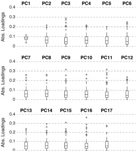
Figure 4 demonstrates how outlier-based selection of important values works for Central LondonRC. The
distribution of loadings for each PC is shown as a box-plot in Figure 4. All PCS, except the first, have a highly skewed distribution of values, and this is indi-cated by the central box (which contains values between the upper and lower quartiles) being posi-tioned toward the lower edge of the plot. The small crosses above the whisker are outliers, and in the case of the loadings they therefore represent the most important destinations. To define important destina-tions for PC1, which has no outliers, we investigated the results in more detail and found that selecting the top 5 percent of loading values for PC1 yields a com-ponent of a similar size to the other PCs.
Step 4: Clustering PCA Scores to Obtain Nonoverlapping Functional Regions
[image:10.594.316.551.55.404.2]At this point in the analysis, Goddard appears to have felt that there was a flaw in his approach, as the resulting regions were overlapping and the PCA did Figure 3. Eigenvalues rank for regions. (A) Central Region and (B) Central and Inner Regions, both using AddLee data.
not result in an exclusive regional assignment (God-dard 1970). He therefore proceeded to derive an alter-native regionalization in which the zones were clustered into groups on the basis of their similarity in the PC score space. That is, the zones were combined based on how “efficient” they were as origins and how they distributed their taxi trips into each PC. In this approach, the scores for each PC were treated as a new, nonspatial data set. Similarity of data points in this new space was then calculated using the Euclidean distance in the attribute space (on scores) and the resulting similarity matrix used in hierarchical cluster-ing. This clustering method starts with every observa-tion as its own cluster and then iteratively joins the two most similar clusters into a larger cluster until all data are grouped together and no more joins are possi-ble (Jain, Murty, and Flynn 1999).
This approach produces a hierarchy of proximity that can be presented as a dendrogram in which they -axis indicates the number of steps after which two sim-ilar clusters can be merged into a larger cluster such that the within-cluster similarity increase is maxi-mized. Cutting the dendrogram at different levels (i.e., at a different number of executed steps of joining the clusters) produces different partitions of the data set into clusters. In contemporary data mining, the level where the dendrogram is cut is normally found by cal-culating internal cluster validation indexes that tell us at what number of clusters the groups are at their most coherent in terms of within-cluster similarity (Everitt et al. 2011). Without access to such algorithms, God-dard (1970) introduced another arbitrary choice by simply cutting his dendrogram at the level that gener-ates twelve clusters. He further created two sets of clusters: one by cutting the dendrogram directly and the other by adding a spatial contiguity criterion that he felt to be necessary, as he was dealing with geo-graphical areas. For the second approach he started with sixty-nine TAZs as individual clusters and at each step merged those two clusters that were the most similar in terms of scores and geographically adja-cent (although again not providing a definition of what this adjacency should mean in geometric terms), thus affecting the similarity order in a way that is, again, not transparent fifty years on.
Because we had initially planned to follow God-dard’s procedure to the letter, we also attempted to execute his last step on our data and were at this point faced with two problems. The first was the choice of dendrogram cut being insufficiently described for repli-cation; the second was the rather unexpected finding
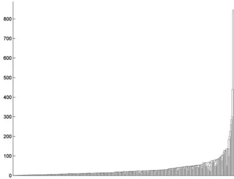
that hierarchical clustering did not in fact reveal any-thing particularly useful about the AddLee flows. Figure 5 shows the dendrogram resulting from the hierarchical clustering of the PC scores in theRIcase. The dendrogram is highly skewed, showing that there are many TAZs that are very similar to each other (and are consequently joined into clusters at the lower numbers of iterations) and a few TAZs that are very different from each other (joined into clusters at the end of the grouping procedure).
[image:11.594.310.542.435.691.2]This means that any cut of the dendrogram will basically split the TAZs into one very large group of TAZs that are broadly similar to each other and a set of very small groups of TAZs that are wildly different from one another. To put it in plainer terms, if we try to cut the dendrogram to obtain two clusters, we get one megacluster and one cluster containing a sin-gle TAZ; if we try to cut the dendrogram to obtain four clusters, then we still find one megacluster and now have three clusters that each contain a single TAZ. This problem exists for at least the first ten clusters extracted from the dendrogram, so we do not consider this outcome to be a meaningful regionaliza-tion and have therefore decided against implement-ing this last step. Consequently, our final result is a set of overlapping functional regions derived directly from Step 3. We further reflect in the Discussion
Figure 4. Distribution of origin loadings for the Central Region (RC).
whether the old requirement of the necessity of there being no overlap between functional regions is still meaningful with the movement patterns of today.
Results
Functional Regions in the Center of London
We now summarize our findings, highlighting the most important regions obtained from our analysis, and relate these to Goddard’s original study. Derived from PC1, Region 1 (shown in Figure 6A) has the densest interconnections between zones serving as important origins and destinations simultaneously. This result points strongly toward a core for AddLee journeys within Central London, and Region 1 is the only grouping that has anything resembling contiguity. In terms of what the region actually represents, the ori-gins are predominantly those of less-connected main-line rail stations to the east and north, and the destinations are predominantly in areas of luxury accommodation and consumption. This aligns well with the characteristics of the AddLee business model. Figure 6B demonstrates the value of this PCA-based approach: Region 2 contains several zones also selected for Region 1, but it is dominated by a strong east–west relationship based on predominantly rich residential origins to the west and walking destinations in the heart of the city or in the emerging agglomeration of consulting and related firms on the South Bank around London Bridge station. In fact, moving down through the remaining fifteen regions shows increased disper-sion, pointing strongly toward a different activity pat-tern from what was captured by Goddard’s black cabs.
Region 3 (Figure 7A) serves to highlight the useful-ness of the ranking that falls naturally out of a PCA-based approach: We know that this region accounts for less variance than Regions 1 and 2 and can infer a narrower type of trip pattern, one undertaken by fewer individuals. In principle, it is possible to disaggregate the journeys underpinning this cluster to better under-stand them, but their spatial location points to non-work activity. A cluster of origins in Kensington and Chelsea is loosely linked with destinations such as King’s Cross station—this journey is not particularly attractive by Tube because of congestion and a num-ber of Tube changes that it requires—and the South Bank. Region 4 captures flows from the northwest of Central London to Waterloo and London Bridge sta-tions, another journey that is more pleasant—if no faster or cheaper—by car.
The remaining regions (see the Supplementary Material) each account for progressively fewer of AddLee’s journeys—recall that the percentage of vari-ance explained can be found in Figure 3. The structure of these regions is, of course, influenced by factors that are not immediately evident from the map: Regions 3 and 4 (see Figure 7), for instance, also join origins and destinations that are relatively weakly connected by London’s Tube system; the routes between them might involve multiple transfers and congestion. Note, how-ever, that the AddLee data reflect a particular set of behaviors, those of cash-rich, time-poor knowledge workers at the top end of London’s income spectrum, so these are not the same functional regions that would emerge from a study of, for instance, London’s omni-present bus system. Moreover, although here we specu-late on the effect of the Tube and the bus system on these two particular regions (3 and 4), it is likely that this effect might be felt and affect the spatial patterns of taxi traffic across all regions. It would, in fact, be very interesting to apply the same methodology on pub-lic transport flows, generated from Tube and bus data, and compare the results with taxi regions. Alterna-tively, there is scope in modeling both taxi and public transport flow data together. All of these analyses, how-ever, constitute their own big data research challenges and are beyond the scope of this article.
Extending the Analysis to the Wider City
[image:12.594.318.549.516.693.2]Turning now to the bigger picture, we briefly inter-pret the larger functional geography of taxi flows as they pertain to both Central and inner London. This
Figure 5. The hierarchical clustering dendrogram of principal component scores for theRIcase.
scale of analysis was simply not possible in the 1960s, so there is an interesting question here as well: Are the patterns produced in the core reproduced at wider scales? Does the link between prestigious residential areas and major transit and employment sites hold, or is there a shift in usage such that functional regions are differently constituted?
In like manner, for the Central and inner set of 391 zones, we extracted the most important PCs, finding
[image:13.594.122.464.57.548.2]nine that contributed more than 1 percent of variance. Figure 8 shows the first two regions of our analysis, and the remainder of the regions are in the online Supple-mentary Materials. As in our first analysis, the first region extracted constitutes an obvious functional cross-cutting core for travel (Figure 8A). It is notable, though, that at this level there is significant in-filling: areas with in- and outflows that were not significant when evaluating only Central London flows. The Figure 6. The Central Region (RC) destinations. (A) The classification into the important origins, destinations, and originsCdestinations from the region derived from the first PC. (B) The same for the region derived from the second PC. Flows belonging to each respective PC are superimposed on the map of zones and shown with varying thickness. PC = principal component. (Color figure available online.)
second region has an altogether different structure (Figure 8B): Although incorporating much of the first functional region as an origin, it has a strong east–west structure incorporating the City and London City Air-port as well as, rather surprisingly, Croydon. Interest-ingly, for the remaining regions (see online Supplementary Materials), many of their origins are zones that are currently poorly served by high-speed links to Central London and to the airports; however, some of these routes will be joined up from 2018 with the launch of the new underground line Crossrail 1 and, eventually, Crossrail 2 services.
In a sense, we can see that London’s structure is still very much monocentric: a slightly engorged central business district (CBD) remains the main draw for— and source of—journeys. The highest value journeys and, by implication, the highest value interactions are still dominated by Central London even if the center derived from AddLee trips is rather larger than a simi-lar study would have found fifty years ago. Overspill of financial activity from the City of London does mean that hedge funds are now principally located in May-fair and to the immediate southwest, whereas success-ful new economy and business services firms can be found from the Old Street Roundabout to Hoxton Square (now rebranded as Tech City), for instance.
A closer consideration of what is actually in the core problematizes this simplistic view. First, the size of the core is rather larger than we would have expected if it were still a traditional style of CBD because it now incorporates a much wider range of functions, including entertainment, leisure, and residential areas. Second, the range of cross-cutting flows is more complex than a simple structure would imply. Within the CBD, the network of flows connects zones to mainline rail sta-tions in much the same way that Goddard (1970) observed in the 1962 data, but it is impossible to isolate each station as a source or sink for a given region even though we recognize that the underlying behavior of AddLee users might play a role in this difference. We also see the densely traversed core spreading westward along the Thames to include tech firms in previously overlooked areas such as Richmond and across the more northerly parts of South London. In short, the core’s persistence across these extracted regions is not purely a function of residential demand.
Conclusions and Discussion
In this article, we have attempted to replicate a some-what forgotten quantitative regionalization methodology
from fifty years ago on modern flow data. We were moti-vated not only by the fact that the old methodology looked suitable for the problem of understanding the city in terms of movement patterns within the urban space, and we wanted to test whether this was the case, but also and perhaps even more by the fact that we believed that we had obtained taxi data from 2011 that were similar to those used in the 1970 study. With these new data we expected to be able to see the change in the functional structure of the city as captured in the movement patterns identifiable in taxi journeys. Although we were able to demonstrate the utility of the old methods, we were not able to fully replicate what had been done in 1970 for var-ious reasons, many of them related to the inevitable social forces that directed how this science was carried out. Here we reflect on our experience and discuss issues that appeared during our replication experiment.
Embarking on this comparison, we quickly found dramatic differences between the kinds of data avail-able then and now. Clearly, the nature of taxi trips in our modern data is different because taxi journeys in 1962 encompassed many more types of trips than those associated with today’s prebooking operators. The rela-tively higher monetary and planning costs of minicab bookings mean that, in a city like London, high-end prebooked services are less likely to be used to pop out to the shops but are common for trips to business meetings or major events. In this sense, our results highlight the extent to which AddLee data are “socially constructed” (Johnston et al. 2014), but as is usual in this type of analysis we have no data on the composition and purposes of journeys for either date. We found, too, that challenges in method replication extend beyond the changing nature of data collection: There are interesting, and potentially worrying, paral-lels between the big data analyses of 1970 and those of 2015. We found ourselves unable to verify crucial details relating to the analysis because both the data and the code—were they even accessible any-where other than in a museum—are simply not machine readable any more.
So can we draw any meaningful comparisons at all? Allowing for the substantial limitations noted earlier, the answer is a qualified “yes.” The most striking differ-ence is the way in which the strongest flows in the sys-tem at both scales are no longer driven primarily by transport; not only are the heaviest flows in the AddLee data over surprisingly short distances but we also see the emergence of strong residential and leisure “poles” at some scales. Obviously, Goddard’s own data did not extend beyond the business core, but although
stations remain important origins and destinations in 2012, there is no longer such a strong sense of in- and outflows and much more cross-cutting behavior. We find no compact regions such as Goddard’s (1970) Fac-tor 1 and FacFac-tor 3, and only more diffuse groups like his Factor 2. The revitalization of the inner city over the intervening fifty years means that the sociocultural and the economic now mix in complex ways (Hutton 2004). Soho and Clerkenwell stand out in several of
[image:15.594.125.465.57.542.2]the PCA-derived regions (Figure 6A) and, when com-bined with AddLee’s business focus, this points toward the type of mixing of work and “play” thought to cre-ate buzz in the contemporary knowledge economy (Storper and Venables 2004). These areas also remain relatively poorly served by heavy transport infrastruc-ture such as London’s Underground and rail network and suggest that taxis are being used to fill in the gaps in a way that Goddard’s black cabs were not.
Figure 7. Two more Central Region (RC) configurations. (A) Classification into the important origins, destinations, and originsC destina-tions from the region derived from the third PC. (B) The same for the region derived from the fourth PC. Flows belonging to each respective PC are superimposed on the map of zones and shown with varying thickness. PCDprincipal component. (Color figure available online.)
Of course, high-value services such as those offered in the City of London and its financial services, and by the specialist legal firms around the Inns of the Court on the Strand, remain heavy drivers of vehicle trips (Figures 6B and 7A), but the most obvious contrast to Goddard’s own results lies in the rising importance of origins and destinations south of the Thames as shown
[image:16.594.133.474.63.575.2]in Figure 7, for example. We can be confident, though, that the biggest differences—had such data been avail-able—would have emerged at the scale encompassed by Figure 8: Canary Wharf and City Airport did not even exist in 1970, but these are now the most prominent travel origins and destinations outside of the business and leisure core. We also see prominent residential Figure 8. The two most important regions from the Inner and Central (RI) analysis. (A) Classification into the important origins, destina-tions, and originsCdestinations from the region derived from the first PC. (B) The same for the region derived from the second PC. Flows belonging to each respective PC are superimposed on the map of zones. PCDprincipal component. (Color figure available online.)
origins in areas such as Fulham, Clapham, and Lad-broke Grove (Figure 8). These reflect a profound trans-formation in the face of Central and inner London. With the exception of Hampstead, in the 1960s these neighborhoods were, for the most part, solidly middle and lower middle class; today, they are bastions of hous-ing for what the London Output Area Classification calls the “Urban Elite” and “City Vibe” demographics (Singleton and Longley 2015). Ultimately, these con-trasts—driven by social, economic, infrastructural, and behavioral factors—help us to grasp the outlines of the underlying transformation of London from declining metropolis to “world city,” but so great is the gulf between these two time periods that like-for-like com-parison is quite simply no longer possible.
On a wider level, however, it should also be noted that our results indicate that older quantitative approaches can continue to shed light on current research challenges. Quantitative methods, like quali-tative ones, go through periods of being in and out of fashion, and we find that in this study the relatively forgotten use of PCA offers specific benefits for flow network analysis over more recent, computationally intensive approaches derived from network science. As we noted earlier, our own attempts employing cut-ting-edge link-clustering approaches required more than a month to complete. Unlike techniques adopted from network analysis (Expert et al. 2011; Thomas et al. 2012), therefore, PCA is able to cope with a highly skewed system of flows, as occurs in the AddLee data set, without producing a trivial partitioning in which most clusters contain a single observation and one cluster contains the rest of the data set. In the context of our data, this corresponds to a trivial core– periphery regionalization in which the entire CBD is disaggregated into separate clusters before anything in the periphery is split into separate groups.
Another issue thrown into relief by our procedure is the persistence of the generally accepted idea that functional regions should be nonoverlapping. Goddard (1970) himself seemed to have felt that an exclusive partitioning was desirable and the hierarchical clustering process, with and without physical contigu-ity constraints, enabled him to create two alternate views of London. There was indeed a strong presump-tion at the time among quantitative geographers that their search was for contiguous and mutually exclusive partitions of space into a clear hierarchy of zones. The idea that unique, contiguous partitions are necessary for interpreting spatial structure has weakened, how-ever, as geographers have accepted that such
hierarchies are no longer likely to be as clear cut, nor as desirable, as was assumed a generation or more ago. In fact, even fifty years ago, it was possible to modify the multivariate methods Goddard used to account for spatial contiguity directly, but this represented the research frontier then and such extensions were not generally available to applied researchers.
There is now a sense that cities benefit from structural complexity and that societies have become more mobile and more able to interact in complex ways, such that the spatial structure of cities is increasingly fragmented into overlapping polycentric forms. Some contemporary realizations of network analysis techniques have taken overlapping structure as an a priori assumption in the regionalization technique (Demsar et al. 2014), but although well known in physics (Ahn, Bagrow, and Leh-mann 2010), they are not yet widely used in geography. That the overlapping regionalization produced by PCA—especially where the concept of regional con-tainment is irrelevant and the desired number of regions is not known—can be an analytical advantage in certain contexts is not commonly recognized today.
The process of polynucleation appears to have taken on special importance in London where districts are highly specialized and contribute to extensive cross-cutting transport and other flows (Hall and Pain 2006). Moreover, results from other metropolitan areas, such as those in central Switzerland, for example (Killer and Axhausen 2009), highlight the fact that overlapping commuting regions in which a single zone contributes to several regions at once could be integral to our understanding of the modern urban landscape. In short, our comparison of central London fifty to sixty years ago with today suggests that there should be a new focus on explaining how spatial structures are continuing to evolve in complex ways. In 1970, God-dard justified his approach using what was then called contact theory, which was an early form of social net-work analysis originating in Sweden from the H€agerstrand School (Warneryd 1968). Our current justification builds on this through new forms of net-work science, multivariate data mining, and transport activity modeling, but the methods for testing and implementing these still strongly resonate with those that were developed in the first quantitative revolu-tion in geography. In the quest to understand the future city, it appears that the tools introduced fifty years ago by researchers such as Goddard will continue to have an important role to play in our understanding of how networks of flows determine the structure of the contemporary city.
Acknowledgements
This work would not have been possible without the support of Addison Lee and Transport for London (TfL), and we would like to recognize their important contribution to this research.
Funding
Jonathan Reades wishes to acknowledge the support of the Engineering and Physical Sciences Research Council (Grant #EP/I018433/1). Jonathan Reades, Urska Demsar, and Michael Batty were supported by the European Commission grant COSMIC: Complex-ity in Spatial Dynamics (ComplexComplex-ity-NET/FP6 ERA-NET) during the early stages of this work. Michael Batty further wishes to thank the European Research Council for support under 249393-ERC-2009-AdG.
Supplemental Materials
The supplemental materials for this article contain maps of all derived functional regions for Central Lon-don (RC) and inner and Central London (RI) and are available on the publisher’s Web site.
ORCID
Urska Demsar http://orcid.org/0000-0001-7791-2807
Jonathan Reades http://orcid.org/0000-0002-1443-9263
Ed Manley http://orcid.org/0000-0002-8904-0513
Michael Batty http://orcid.org/0000-0002-9931-1305
References
Ahn, Y. Y., J. P. Bagrow, and S. Lehmann. 2010. Link com-munities reveal multi-scale complexity in networks.
Nature466:761–65.
Batty, M. 2013. The new science of cities. Cambridge, MA: MIT Press.
Berry, B. J. L. 1964. Approaches to regional analysis: A syn-thesis.Annals of the Association of American Geographers
54:2–11.
———. 1970. The geography of the United States in the year 2000.Transactions of the Institute of British Geogra-phers51:21–53.
Berthold, M., and D. J. Hand. 2007.Intelligent data analysis. Berlin: Springer Verlag.
Bettencourt, L., and G. West. 2010. A unified theory of urban living.Nature467:912–13.
Black, W. R. 1973. Toward a factorial ecology of flows.
Eco-nomic Geography49:59–67.
Castells, M. 1996. Rise of the network society. New York: Wiley-Blackwell.
Daultrey, S. 1976. Principal components analysis. Norwich, UK: Geo Abstracts, University of East Anglia.
Davies, W. K. D. 1979. Urban connectivity in Montana.
The Annals of Regional Science13 (2):29–46.
Demsar, U., P. Harris, C. Brunsdon, A. S. Fotheringham, and S. McLoone. 2013. Principal component analysis on spatial data: An overview.Annals of the Association
of American Geographers103:106–28.
Demsar, U., J. Reades, E. Manley, and M. Batty. 2014. Edge-based communities for identification of functional regions in a taxi flow network. Paper presented at the 8th International Conference on Geographic Informa-tion Science, Vienna, Austria.
Demsar, U., O. Spatenkov a, and K. Virrantaus. 2007. Centrality measures and vulnerability of spatial net-works. Paper presented at the 4th International Conference on Information Systems for Crisis Response and Management, ISCRAM 2007, Delft, The Netherlands.
Everitt, B. S., S. Landau, M. Leese, and D. Stahl. 2011.
Cluster analysis. 5th ed. New York: Wiley.
Expert, P., T. S. V. D. Evans, V. D. Blondel, and R. Lambiotte. 2011. Uncovering space-independent com-munities in spatial networks.Proceedings of the National Academy of Sciences of the United States of America
108:7663–68.
Farmer, C. J. Q., and A. S. Fotheringham. 2011. Network-based functional regions. Environment and Planning A
43:2723–41.
Goddard, J. B. 1970. Functional regions within the city cen-tre: A study by factor analysis of taxi flows in Central London. Transactions of the Institute of British
Geogra-phers49:161–82.
———. 1973. Office linkages and location: A study of com-munications and spatial patterns in Central London.
Progress in Planning1:109–232.
Hall, P. 2009. Looking backward, looking forward: The city region of the mid-21st century. Regional Studies 43 (6):803–17.
Hall, P., and K. Pain, eds. 2006.The polycentric metropolis:
Learning from mega-city regions in Europe. London:
Earthscan.
Harris, R. J. 2001.A primer of multivariate statistics. Mahwah, NJ: Erlbaum.
Hutton, T. A. 2004. The new economy of the inner city.
Cities21 (2):89–98.
Illeris, S., and P. O. Pedersen. 1968. Central places and functional regions in Denmark: Factor analysis of tele-phone traffic.Geografisk Tidsskrift67:1–17.
Jain, A. K., M. N. Murty, and P. J. Flynn. 1999. Data clus-tering: A review.ACM Computing Surveys (CSUR)31: 264–323.
Johnston, R., R. Harris, K. Jones, D. Manley, C. E. Sabel, and W. W. Wang. 2014. One step forward but two steps back to the proper appreciation of spatial science.
Dia-logues in Human Geography4:59–69.
Jolliffe, I. T. 2002. Principal component analysis. Berlin: Springer Verlag.
Kaiser, F. H. 1958. The varimax criterion for analytic rotation in factor analysis.Psychometrika 23:187–200. Killer, V., and K. W. Axhausen. 2009. Mapping overlapping commuting areas.Arbeitsberichte Verkehrs-und Raumpla-nung 555. Accessed October 25, 2017. https://doi.org/ 10.3929/ethz-a-005800372
Nielsen, T. A. S., and H. H. Hovgesen. 2008. Exploratory mapping of commuter flows in England and Wales.
Journal of Transport Geography16:90–99.
O’Sullivan, D., and Manson, S. M. 2015. Do physicists have “geography envy”? And what can geographers learn from it? Annals of the Association of American
Geogra-phers105 (4):704–22.
Ratti, C., S. Sobolevsky, F. Calabrese, C. Andris, J. Reades, M. Martino, R. Claxton, and S. H. Strogatz. 2010. Redrawing the map of Great Britain from a network of human interactions.PLoS ONE5:e14248.
Reades, J., and D. A. Smith. 2014. Mapping the “space of flows”: The geography of global business telecommuni-cations and employment specialization in the London mega-city-region.Regional Studies48:105–26.
Rogerson, P. A. 2006. Statistical methods for geography: A student’s guide. London: Sage.
Roth, C., S. M. Kang, M. Batty, and M. Barthelemy. 2011. Structure of urban movements: Polycentric activity and entangled hierarchical flows. PLoS ONE
6:e15923.
Rummel, R. J. 1967.Understanding factor analysis. Honolulu: Social Science Research Institute, Department of Polit-ical Science, University of Hawaii.
Singleton, A. D., and P. Longley. 2015. The internal struc-ture of Greater London: A comparison of national and regional geodemographic models. Geo: Geography and
Environment2 (1):69–87.
Storper, M., and A. J. Venables. 2004. Buzz: Face-to-face contact and the urban economy. Journal of Economic
Geography4 (4):351–70.
Tanaka, Y., and F. Zhang. 1999. R-mode and Q-mode influ-ence analyses in statistical modelling: Relationship between influence function approach and local influ-ence approach.Computational Statistics and Data Analy-sis32:197–218.
Taylor, P. J., D. Evans, and K. Pain. 2006. Organisation of the polycentric metropolis: Corporate structures and networks. In The polycentric metropolis: Learning from
mega-city regions in Europe, ed. P. Hall and K. Pain,
53–64. London: Earthscan.
Thomas, I., C. Cotteels, J. Jones, and D. Peeters. 2012. Revisiting the extension of the Brussels urban agglom-eration: New methods, new data. . .new results?Belgeo
1–2:1–12.
Voorhees, A. M. [1954] 2013. A general theory of traffic movement (The 1955 ITE Past Presidents Award paper).Transportation40:1105–16.
Warneryd, O. 1968. Interdependence in urban systems. G€oteborg, Sweden: Regionkonsult Aktie-Bolag. Zheleva, E., and L. Getoor. 2007. Preserving the privacy of
sensitive relationships in graph data. In Proceedings of the 1st ACM SIGKDD International Conference on Pri-vacy, Security, and Trust in KDD, ed. F. Bonchi, E. Fer-rari, B. Malin, and Y. Saygin, 153–71. Berlin-Heidelberg: Springer Verlag.
Zhong, C., S. M. Arisona, X. Huang, M. Batty, and G. Schmitt. 2014. Detecting the dynamics of urban structure through spatial network analysis.International Journal of Geographical Information Science28:2178–99.
URSKA DEMSAR is Lecturer (Assistant Professor) at the School of Geography & Sustainable Development, Uni-versity of St. Andrews, St. Andrews KY16 9AL, Scotland, UK. E-mail: [email protected]. Her research area is spatiotemporal visual analytics with a specific focus on computational movement analysis. She collaborates with movement researchers in a number of application areas, including eye tracking, human dynamics, and ani-mal movement.
JONATHAN READES is Lecturer in the Department of Geography, King’s College London, Strand, London WC2R 2LS, UK. E-mail: [email protected]. His key research interests are in social and economic networks; firm location, innovation, and growth; the impact of embedded, networked technologies on urban environments (“smart cit-ies”); and big data from digitally enabled communications and transportation networks
ED MANLEY is Lecturer at the Centre for Advanced Spa-tial Analysis at University College London, London WC1E 6BT, UK. E-mail: [email protected]. His research focuses on the use of new forms of transportation data to better understand and model mobility behavior. Through this research theme, he has developed novel insights into travel behavior using smart card data, mobile phone trans-action data, and the route choice behaviors of minicab drivers.
MICHAEL BATTY is Bartlett Professor of Planning at the Centre for Advanced Spatial Analysis at University College London, London WC1E 6B, UK. E-mail: [email protected]. His research focuses on the development of large-scale urban simulation models and their visualization and he has worked extensively on methods of spatial analysis that support such applications.