Intuitive and Reliable Estimates of Output Gap and Real Exchange Rate Cycles for Turkey

Munich Personal RePEc Archive

Intuitive and Reliable Estimates of

Output Gap and Real Exchange Rate

Cycles for Turkey

Ekinci, Mehmet Fatih

Atilim University

25 June 2019

Online at

https://mpra.ub.uni-muenchen.de/94698/

Intuitive and Reliable Estimates of Output Gap and Real Exchange Rate Cycles for Turkey∗

Mehmet Fatih Ekinci∗

Abstract

Decomposing time series data into trend and cyclical components is among the top priorities for

policy maker institutions. Comparing with the unrestricted Beveridge-Nelson decomposition and

Hodrick-Prescott filter, we implement a restricted Beveridge-Nelson filter developed by Kamber et.

al. (2018) which limits the volatility of trend component. Utilizing the quarterly real GDP series

and monthly real exchange rate data for Turkey, we find that Beveridge-Nelson filter provides more

persistent and larger cyclical values than Beveridge-Nelson decomposition. Taking the output gap

estimates of Central Bank of Turkey as a benchmark, our results indicate that Beveridge-Nelson

filter method yields more sensible results. We also develop a measure to make an assessment on

the end-point bias. Our results show that restricted Beveridge-Nelson filter performs better than

Hodrick-Prescott filter regarding the magnitude of end point bias.

Keywords: Beveridge-Nelson decomposition, Beveridge-Nelson filter, Hodrick-Prescott filter, output gap, real exchange rate cycles, signal-to-noise ratio.

JEL Codes: C22 Time Series Models, E17 Forecasting and Simulation: Models and Applications, E32 Business Fluctuations Cycles, F31 Foreign Exchange.

∗

1. Introduction

Estimating a robust and stable trend is an important challenge for economic analysis. To

this end, output gap, which can be defined as the difference between the actual output and its

“potential” level, is closely monitored by the central banks for the implementation of the monetary

policy. Several methods have been developed to estimate the output gap2_{. Results from these}

studies suggest that cyclical component of output has a large amplitude and persistent behaviour.

Along with the interpretation of business cycles, a detrending method which yields small and noisy

cycles can be classified as counter-intuitive.

Furthermore, many methods developed to estimate cyclical values suffer from an end-point

problem, which might be characterized by the exaggerated impact of the terminal data point. If

the purpose of the analysis is to document and study the properties of the cyclical component,

one can simply omit the terminal data points of the series. On the other hand, if the trend is

used for policy purposes, then the terminal data point is likely to be the one which is particularly

interesting. If the difference between real time estimates and estimated values with addtional

data points display a divergence, then the estimation method can not be considered as a reliable

technique.

Since the trend component is defined by a conditional expectation of the permanent component,

Beveridge-Nelson (BN) decomposition is a prominent method of estimating cyclical values for an

integrated time series. Regarding these intuitiveness and reliability issues, Kamber et. al. (2018)

shows that when lag structure is determined by information criteria, standard BN decomposition

produces small and noisy output gap estimates. They develop a restricted version of BN

decompo-sition with a strong prior belief that the volatility of the cyclical component is much higher than

the one of the trend component. This adapted filter produces sensible estimates of the US output

gap that are reliable, intuitive, subject to less revisions and which moves closely with the National

Bureau of Economic Research (NBER) business cycle.

In this study, we describe unrestricted BN decomposition and the restricted BN filter developed

by Kamber et. al. (2018). Using quarterly GDP data for Turkey, we implement these methods.

Taking the official estimates provided by Central Bank of Turkey as a benchmark for output gap,

2

we compare the performance of these methods. We include the popular Hodrick-Prescott (HP)

filter as an alternative for this exercise. We find that BN decomposition provides small and noisy

cycles. Estimates from HP filter are persistent and exhibit a larger amplitude, but suffer from a

large end point bias problem. BN filter method dominates the alternatives by producing intuitive

and reliable estimates of output gap. When we conduct the same exercise utilizing the monthly

real exchange rate (RER) series for Turkey, our results remain intact.

The paper is organized as follows. Next section describes BN decomposition, section 3 explains

the BN filter developed by Kamber et. al. (2018). In section 4, we focus on the persistence and

amplitude of cycles obtained by applying BN decomposition and BN filter on the real GDP data

for Turkey. We compare our results with HP filter cycles and focus on the intuitiveness of BN filter

cycles. Section 5 provides a dicussion on the reliability of BN filter by investigating the end-point

bias observed in BN filter output gap estimates. Section 6 dscusses the RER cycles obtained with

BN filter. Finally, section 7 concludes.

2. Beveridge-Nelson (BN) Decomposition

Following Beveridge and Nelson (1981), we express an integrated time series as the sum of two

components,

yt=τt+ct (1)

where τt represents the long-run trend which follows a random walk with a drift, and ct denotes

the cyclical component. Trend component in BN decomposition is defined as the infinite horizon

expectation of the time series: τt ≡ limh→∞Et[yt+h−h µ] where µ is the drift term. Since yt is

an I(1) process, the first difference of the series is stationary. We define the deviation from the

unconditional mean as ∆˜yt ≡ (∆yt−µ). To illustrate the BN decomposition for a simple case,

suppose that the first difference can be expressed as an AR(1) process given by,

∆˜yt=φ1∆˜yt−1+et (2)

where|φ1|<1 andet∼i.i.d.N(0, σ2). For this process, the trend component is,

τt = yt+

φ1

1−φ1

Given the trend, cyclical component is

ct = −

φ1

1−φ1

∆˜yt (4)

Considering the generalized case, suppose that the first difference of data series is characterized by

an ARMA(p,q) process described as,

φ(L)∆˜yt=θ(L)et, (5)

where φ and θ are autoregressive and moving-average polynomials in the lag operator L, respec-tively. We can write this model in the state space form to calculate the cyclical component. Transition equation is

              

∆˜yt ∆˜yt−1

∆˜yt−2

...

∆˜yt−p+1

et

et−1

et−2

... et−q+1

              

p+q×1

=               

φ1 φ2 ... φp−1 φp θ1 θ2 θ3 ... θq−1 θq 1 0 ... 0 0 0 0 0 ... 0 0 0 1 ... 0 0 0 0 0 ... 0 0

... ... ... ... ... ... ... ... ... ... ...

0 0 ... 1 0 0 0 0 ... 0 0 0 0 ... 0 0 0 0 0 ... 0 0 0 0 ... 0 0 1 0 0 ... 0 0 0 0 ... 0 0 0 1 0 ... 0 0

... ... ... ... ... ... ... ... ... ... ...

0 0 ... 0 0 0 ... 1 0

              

p+q×p+q

              

∆˜yt−1

∆˜yt−2

∆˜yt−3

...

∆˜yt−p

et−1

et−2

et−3

... et−q

              

p+q×1

+                et 0 0 ... 0 et 0 0 ... 0               

p+q×1

More compactly, we can write the transition equation as follows,

Xt=F Xt−1+νt (6)

whereνt∼ N(0,Ω). Measurement equation is

∆˜yt=HXt= [1 0...0]Xt (7)

Minimum MSEj-period ahead forecast is given by

Et[∆˜yt+j] =HFjEt[Xt] (8)

The state vector contains some unobserved elements, and Kalman filter provides this expectation

under a normality assumption. Following Morley(2002), Beveridge-Nelson cycle can be calculated

as

To analyze the share of cyclical fluctuations in the series, we define a signal to noise ratio. To

express this ratio, a Wold representation of the underlying ARMA(p,q) process is more useful

∆yt=µ+ψ(L)et (10)

In this case, trend component can be expressed as,

τt=µ t+ψ∗(1) t

X

s=1

es (11)

where long-run multiplier for our ARMA(p,q) process is

ψ∗(1) = 1 +θ1+θ2+...+θq 1−φ1−φ2−...−φp

(12)

Signal to noise ratio for BN decomposition is defined as the variance of trend shocks as a fraction

of overall forecast error variance,

δ≡ σ

2 ∆τ

σ2

e

(13)

Using the results from the Wold representation above, signal to noise ratio is,

δ ≡ψ∗(1)2 (14)

which indicates that signal to noise ratio is the square of the long run multiplier obtained from

Wold representation.

3. BN Filter

Different approaches to estimate output gap yield different results which might potentially

have conflicting policy implications. A popular method developed by Hodrick and Prescott (1980)

produces large and highly persistent cycles. However, HP filter estimates suffer from end-point

bias and updated estimates after data revisions cast doubt on the reliability of this method. On

the other hand, BN decomposition typically gives small and noisy cycles.

To reconcile these differences, Kamber et al. (2016) investigate how one can generate large

cyclical components using the BN decomposition. They find that by setting the noise-to-signal

ratio to be large, instead of estimating it from the data, the cycles obtained are large and the

From a technical perspective, BN filter relies on the insight that signal to noise ratio depends

on the autoregressive coefficients of an AR(p) model. This result yields the conclusion that we can

fix the signal to noise ratio by restricting the autoregressive coefficients. Considering an AR(p)

model given by

∆˜yt=φ1∆˜yt−1+φ2∆˜yt−2+...+φp∆˜yt−p+et (15)

which can be rearranged as follows,

∆˜yt=ρ∆˜yt−1+

p−1

X

j=1

φ∗_j∆˜yt−j+et (16)

where ρ ≡φ1+φ2+...+φp = 1−φ(1) and φ∗j ≡ −(φj+1+...+φp). Then, AR(p) model given

above can be estimated by restricting signal to noise ratio ¯δ as follows,

¯

ρ= 1−1/pδ¯ (17)

Value for AR(p) coefficients are fitted by utilizing a “Minnesota” type shrinkage prior on the higher

lags of the model where

φ∗j ∼ N(0, 0.5

j2 ) (18)

Conditional on σ2_e, the posterior distribution for nφ∗_jop−

1

j=1 has a closed-form solution and can be

calculated without the need for posterior simulation. In practice, number of lags is set to 12,

p= 12. Defining the implied amplitude to noise ratio,

α(δ)≡ σ

2

c(δ)

σ2

e(δ)

(19)

¯

δ is chosen to maximize this ratio as follows,

¯

δ=inf

δ >0 :α′(δ)>0, α′′(δ)<0 (20)

The procedure can be summarized in 3 steps as follows,

1. Set a low ¯δ. Repeat step 2 and 3 for incremental increases in ¯δ from an initial increment just

above zero until the estimatedα(¯δ) decreases.

n φ∗

j

op−1

j=1 by setting p = 12.

3. Given ¯δ and estimates ofnφ∗

j

op−1

j=1 , solve for restricted estimates of{φj}

p−1

j=1 by applying the

BN decomposition.

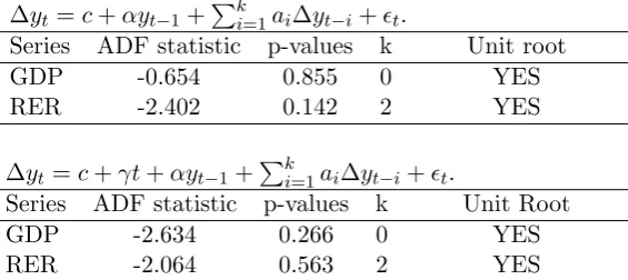
To apply the BN decomposition and BN filter, we verify the existence of a unit root in our

sample. Results from augmented Dickey-Fuller tests on the output and real exchange rate series are

reported in Table 1. We cannot reject the unit root hypothesis for both output and real exchange

rate series for Turkey. Thus, we conclude that presence of stochastic trends in the data series

motivate the application of Beveridge Nelson decomposition and BN filter.

4. Persistence and Amplitude of Output Gap for Turkey

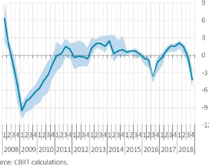
In order to make an assessment on the performance of BN filter, we present the output gap

estimates of Central Bank of Turkey (CBRT) in figure 1 as a benchmark. The sample of official

estimates covers the period between 2008Q1 and 2018Q4. We observe that output gap exhibits a

persistent behaviour. Amplitude of the estimates is quite large, reaching a trough around 9 percent

in 2009Q1 during the global economic crisis.

Output gap is estimated by using BN decomposition, BN filter and HP filter utilizing the

quarterly GDP data3 _{for Turkey between 1960Q1 and 2018Q4. We compare our results with the}

CBRT estimates in order to understand whether these methods provide sensible and intuitive

results. For BN decomposition, we select a lag length based on Schwartz Information Criteria

(SIC) which suggests an AR(1) model. When BN filter is utilized, estimated signal to noise ratio

for GDP series is 0.14.

Persistence and standard deviation of the output gap estimates are reported in table 2. Cyclical

component obtained with BN decomposition exhibits a smaller amplitude and weaker persistence.

HP filter and BN filter both produce persistent output gap estimates with a larger amplitude

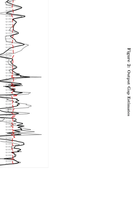
compared to the BN decomposition. Figure 2 plots the output gap estimates obtained with these

alternative methods. BN filter and HP filter cycles move closely for most of the sample with a

correlation of 0.70. We observe that the dates of negative values roughly coincide with the estimates

3

published by CBRT (2019) for both methods. The size of the trough in 2009Q1 is quite close to

the official estimates for BN filter (7.41 percent) and HP filter (8.40 percent). Sign and direction

of the estimated cycles are consistent with the official estimates.

5. Reliability of Output Gap Estimates

Our analysis suggests that BN filter and HP filter methods provide large and persistent output

gap estimates. We can consider that implementing these methods yield intuitive estimates of

output gap. Another important aspect of extracting a robust and stable trend is the difference

between the estimated values when additional data points are available and the real time estimates.

Choosing the appropriate filtering method is particularly important as information on the future

path of the economy is missing when the policy decisions are made. Value of trend in the terminal

period is based on the information available up to and including the terminal period4_{. Therefore, it}

might change significantly when new data become available, irrespective of whether the new data

point is driven by cyclical or structural factors.

We estimate the cyclical component for the last decade of our sample5 _{recursively by using the}

full sample and cutting the sample at the data point. We define the measure of end-point bias as

follows,

end-point-bias_t≡ct|t−ct|T (21)

where ct|t is the real time estimate of cyclical component and ct|T is the output gap obtained by

using full sample. Table 3 reports the standard deviation and average of the absolute value of the

bias. The magnitude of end-point bias is quite large for HP filter. The results indicate that BN

filter dominates HP filter in terms of providing a reliable estimate of Turkish output gap.

6. Real Exchange Rate (RER) Cycles for Turkey

Our exercise using quarterly real GDP series shows that BN filter dominates HP filter and BN

decomposition in terms of providing intuitive and reliable output gap estimates. We extend our

4

There is also a very important discussion on the sensitivity of business cycle facts to the filtering methods used. Canova (1998) reports that stylized facts about the US economy vary widely across different detrending methods.

5

analysis by utilizing monthly real exchange rate series to compare these alternative methods to

estimate cyclical values6_{. This exercise also relates to the permanent equilibrium exchange rate}

(PEER) literature. In this literature, the trend of the real exchange rates series is defined to be a

long-run equilibrium value and the cyclical component is referred as deviations from equilibrium

real exchange rate or real exchange rate misalignments.

In this case, information criteria suggests an AR(2) model for BN decomposition. Estimated

signal to noise ratio for RER series is 0.16 with BN filter. Cyclical values estimated with alternative

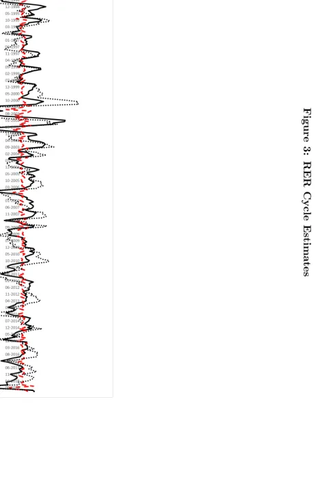
methods are plotted in figure 3. Persistence and standard deviations are reported in table 4. Our

results show that BN decomposition yields counter-intuitive cyclical values in this case as well.

BN filter and HP filter provides persistent and large RER cycles. The estimates obtained from

these methods move closely with a correlation coefficient of 0.71. When we compare these two

methods in terms of the magnitude7 _{of the end-point bias, BN filter dominates HP filter in terms}

of reliability. Standard deviations and average absolute values of bias are reported in table 5.

7. Conclusion

Decomposing economic time series into trend and cyclical components is among the top

pri-orities of economists. Several methods have been developed to extract the cyclical component of

the data. Real-time allocation of structural and cyclical dynamics is essential, especially for policy

analysis. For example, estimating a reasonably accurate output gap is an important task for

pol-icy maker institutions, especially central banks. Central bankers would like to know the size and

direction of the gap between actual and potential GDP, so as to determine whether the economy

needs more or less monetary stimulus. A particularly important task is to reconcile the differences

between estimation methods. Estimates obtained from appropriate detrending methods can be

useful to conduct a real time analysis if the announcement of new data is within a reasonable time

frame. The results can also be utilized to conduct analysis on the economic dynamics, such as

Philips curve and Okun’s law.

This study describes and implements BN decomposition along with a restricted BN filter

devel-oped by Kamber et. al. (2018). We use quarterly GDP data and monthly RER series for Turkey.

We take the official estimates provided by Central Bank of Turkey as a benchmark for output gap

6

See Ekinci et. al. (2013) for an application of alternative filtering methods on the Turkish RER data.

7

and conduct our exercises by comparing our results with HP filter estimates. Results show that

BN decomposition provides small and noisy cycles for both series. Estimates from HP filter are

persistent and exhibit a larger amplitude, but suffer from a large end point bias problem. BN filter

method dominates these alternatives by producing intuitive and reliable estimates of output gap

References

[1] Alp, H., ¨O˘g¨un¸c, F. and Sarıkaya, C¸ . [2012], “Monetary policy and output gap: Mind the composition”, Central Bank of Turkey Research Notes in Economics, 2012-07.

[2] Beveridge, S. and Nelson C. [1981] “A new approach to the decomposition of economic time series into per-manent and transitory components with particular attention to measurement of the business cycle”, Journal of Monetary Economics 7, 151174.

[3] Canova, F. [1998], “Detrending and turning points”, Journal of Monetary Economics, vol. 41, 475-512. [4] CBRT [2019], Central Bank of Turkey Inflation Report, 2019-II.

[5] Ekinci, M. F., Kaba¸s, G. and Sunel, E., [2013], “ End-Point Bias in Trend-Cycle Decompositions: An Appli-cation to the Real Exchange Rates of Turkey”, Central Bank Review, vol. 13(3), pages 61-71.

[6] Hodrick, R. and Prescott, E. [1980], “Postwar U.S. Business Cycles: An Empirical Investigation”, Carnegie Mellon University discussion paper no. 451.

[7] Kamber, G., Morley, J. and Wong, B. [2018], “Intuitive and Reliable Estimates of the Output Gap from a Beveridge-Nelson Filter”, The Review of Economics and Statistics 2018 100:3, 550-566.

[8] Morley, J. [2002], “A state-space approach to calculating the Beveridge-Nelson decomposition”, Economics Letters, Elsevier, vol. 75(1), pages 123-127.

[9] ¨O˘g¨un¸c, F. and Ece, D. [2004] “Estimating the output gap for Turkey: an unobserved components approach”, Applied Economics Letters, 11(3),177-182.

[10] ¨Ozbek, L. and ¨Ozlale, ¨U. [2005], “Employing the extended Kalman filter in measuring the output gap”, Journal of Economic Dynamics and Control, 29(9), 1611-1622.

Table 1: Unit Root Tests

∆yt=c+αyt−1+P_ik=1ai∆yt−i+ǫt.

Series ADF statistic p-values k Unit root

GDP -0.654 0.855 0 YES

RER -2.402 0.142 2 YES

∆yt=c+γt+αyt−1+Pk_i=1ai∆yt−i+ǫt.

Series ADF statistic p-values k Unit Root

GDP -2.634 0.266 0 YES

RER -2.064 0.563 2 YES

Notes: GDP is the seasonally adjusted annual levels of quarterly series by OECD in 2010 TL prices. GDP series cover the period between 1960Q1 and 2018Q4. RER is the trade weighted real ef-fective exchange rate index for Turkey. RER is calculated by Bank for International Settlements and covers the period between January 1994 and December 2018. Top panel reports the unit root tests with an intercept term, and bottom panel includes a time trend. Natu-ral logarithms of series are used in the regressions. Lag lengths are chosen by Schwarz information criteria.

Table 2: Persistence and Amplitude of Output Gap Series

Autocorrelation Standard Deviation

BN AR(1) 0.106 0.236

BN Filter 0.803 2.171

HP Filter 0.783 2.921

Table 3: End-Point Bias for Output Gap Estimates

BN Filter HP Filter Standard Deviation 0.108 2.937 Average Abs. Value 0.081 2.255

Notes: End point bias is defined as the difference between real time estimates and cyclical values when full sample is utilized. Standard deviations and average absolute values for 2008Q1-2017Q4 period are reported.

Table 4: Persistence and Amplitude of RER Cycles

Autocorrelation Standard Deviation

BN AR(2) -0.200 1.209

BN Filter 0.833 5.165

HP Filter 0.792 6.661

Notes: Autocorrelation and standard deviation for estimated cyclical values are reported for different estimation methods.

Table 5: End-Point Bias for RER Cycle Estimates

BN Filter HP Filter Standard Deviation 0.234 2.765 Average Abs. Value 0.359 2.571

F igu re 2: O u tp u t G ap E st im at e s

-15 -10 -5 0 5 10

F igu re 3: R E R C y c le E st im at e s