Munich Personal RePEc Archive
Threshold Effect of Scale and Skill in
Active Mutual Fund Management
Chong, Terence Tai Leung and Lee, Nayoung and Sio,
Chan-Ip
30 July 2018
1
Threshold Effect of Scale and Skill
in Active Mutual Fund Management
Terence Tai-Leung Chong
a, Nayoung Lee
b, and Chan-Ip Sio
cJuly 2018
Abstract
In this paper, we apply threshold estimation techniques to study the size-performance relation in the US mutual fund industry. The existing studies have found diseconomies scale, and we add our contribution to this by considering possible non-linear decreasing returns to scale caused by fund age and manager tenure. We find significant threshold effects of both fund age and manager tenure at approximately three to four years in the size-performance relation. Compared with younger funds, older funds have severe decreasing returns to scale as the industry size increases.
JEL Classifications: C24, G11, G23, J24
Keywords: Active mutual funds management, Returns to scale, Threshold estimation
a
Terence Tai-Leung Chong: Department of Economics, The Chinese University of Hong Kong, email: [email protected]
b
Nayoung Lee: Department of Economics, University of Cincinnati, email: [email protected] c
2
1.
Introduction
The size effect on active mutual fund performance has long been studied, and a number of
studies have reported decreasing returns to scale. At the fund level, Berk and Green (2004) argue
that fund performance deteriorates because of the increase in various trading costs and of the
decrease in returns to scale brought by huge capital inflow. Chen et al. (2004) find an evidence of
fund-level decreasing returns and argue that low liquidity is the major cause of the diseconomies
of scale. Pástor et al. (2015) first investigate industry-level size effect and conclude decreasing
returns to scale as the fund industry size grows.
In this paper, we focus on the threshold effect of industry size on fund performance. We
explore potential difference in fund size effects with respect to fund age and tenure of fund
managers. This is motivated by the findings in Pástor et al. (2015) that younger funds outperform
older funds with better skills. Pástor et al. argue that active mutual fund industry has become
more skilled over time but the upward trend in skill coincides with industry growth which makes
it harder for fund managers to outperform.
If younger funds have superior features including the avoidance of competition by new
strategies that differ from those of incumbents, younger funds may experience lesser degrees of
erosion in a crowded industry than older funds. We examine this hypothesis by investigating the
difference in the returns to scale between young and old funds based on the threshold model
3
estimate a threshold model for the US actively managed equity mutual fund market from 1979 to
2013. The advantage of our model is that it can define young and old funds endogenously.
Our results show that the thresholds exist for both fund age and manager tenure at
approximately three to four years. More importantly, young funds experience less performance
erosion than old funds in all regression specifications and samples. These findings are consistent
with the hypothesis that new entrants are managed by a more knowledgeable investment team
than existing funds are. Young funds tend to be less affected by an increasing industry size
compared with old funds. Such results remain statistically significant after controlling for fund
size and other fund liquidity factors. Hence, differences in liquidity characteristics could not fully
explain the lower sensitivity of young funds to the increase in industry size. Our findings are
consistent with the studies which argue required skills in financial industry (e.g. Philippon and
Reshef, 2012); young funds may benefit from better education and knowledge about relevant
technology of fund management experts.
The rest of this paper is organized as follows. Section 2 introduces our main methodology.
Section 3 describes the data. Section 4 presents our empirical results and discusses related issues.
Section 5 concludes the paper.
2.
Methodology
4
We first consider a fixed effect (FE) model without threshold to investigate the size-performance:
GrossRit aiInduSizet1it,
where GrossRit is the monthly return of fund i in period t that is adjusted on the basis of the
three-factor model of Fama and French (1997), plus the monthly expense ratio.1 InduSizet-1 is
the size of the active mutual fund industry and measured by the lagged ratio of the sum of assets
under management (AUM) of all funds to the aggregate asset value of the US stock market. Here,
ai is the fixed effect, which measures investment skill of fund managers. The effects of industry
size on mutual fund performance is therefore captured by β. A negative β represents inverse
relationship between the scale of industry sizeand fund returns.
Fund size can be added to the model to control for the fund size effect:
GrossRit ai1InduSizet12FundSizeit1it,
where FundSizeit-1is the lagged value of the AUM of fund i. The reason for introducing ai in
previous models is to control for unobserved characteristics of funds. If ordinary least
squares (OLS) specifications without fund FEs ai are used, omitted variable bias emerges
because of the potential relation between the unobserved effects of skills of fund managers
and fund flows.2 The FE model reduces the effects of this problem. However, another bias
related to β2 may exist because of the demeaning procedures in the OLS‐FE model, as
1
The expense ratio reflects the raw performance of a fund in the market before distribution to clients. 2
5
mentioned by Chen et al. (2004). To address the second bias, Pástor et al. (2015) employ
the recursive demeaning (RD) method by Hjalmarsson (2010). Such bias will not be
discussed in the study given that the effect of fund size is not our core interest. This RD
approach is used only when fund size is included in the regression.3
2.2
Threshold Model
Our key interest is to investigate the difference in the performance erosion of young and old
funds under industry competition. To define young and old funds endogenously, we apply the
threshold model of Hansen (1999). Our threshold model is as follows:
GrossRit ai
1InduSizet1I(dit1
)
2InduSizet1I(dit1
)
it,where dit-1is either the fund age or fund manager tenure measurement for distinguishing between
young and old funds. Thus, β1 and β2 represent the effects of industry size on the performance of
a fund before and after the threshold γ, respectively.
Fund age refers to the period since a fund was launched. It is a common measurement of
how old a fund is. Manager tenure (denoted by MgrTenure) refers to how long a manager
manages a fund. Every new management is considered as a form of rebirth because a new
manager may alter fund portfolios according to his or her investment philosophy. Therefore, a
3
6
fund can be regarded as a young fund when management changes. The period when a current
manager takes control is thus used as another fund age measurement.
MgrTenure is, however, not an ideal measurement of a fund manager’s experience, which
should be related closely to the individual’s age, education, or experience in the financial
industry. In the succeeding sections, MgrTenure cannot yield robust conclusions in some cases.
Considering the data availability, MgrTenure remains a candidate for age measurement.
Our threshold effect is embedded in the original FE model. The FE model identifies the
variation of performance and size within a fund. In the FE model, the coefficients β1 and β2
represent the effects of industry size on a fund’s performance before and after the threshold,
respectively. According to this identification strategy, when fund age exceeds the threshold,
industry size effect significantly affects fund returns. Such effect can be measured by the
difference between β1 and β2.
The estimation is implemented on the basis of the work of Hansen (1999). γ is estimated
as
ˆ
arg minS() ,
where S(γ) is the sum of squared errors (SSE) of the OLS estimation. To obtain the estimate, we
sort the value of the threshold variables in our sample and obtain 400 quantiles in increasing
7
the smallest value of SSE. Finally, the estimators of betas are evaluated at the estimated
threshold:
ˆ
ˆ
( ˆ
)
.3.
Data
The mutual fund data that support the findings of our study are obtained from the CRSP
Survivor-Bias-Free US Mutual Fund Database which is openly available in the center for
research in security Prices (CRSP) at http://www.crsp.com/products/research-products/
crsp-survivor-bias-free-us-mutual-funds.We mainly follow the steps implemented by Pástor et al.
(2015) in cleaning the data4, except for the merging of the two data sets (CRSP and Morningstar
databases) and determining their commonalities.5
We first select observations of open-end active management funds in the US equity market.
Only observations in CRSP with documented fund styles, cap-based domestic equity and
style-based domestic equity, are selected in our sample to reflect the overall situation of equity
mutual fund market. Bond funds, money market funds, international funds, funds of funds, and
retirement target funds are excluded from the sample because our priority is to focus on the
4
Pástor et al. (2015) followed the data cleaning procedures of Berk and Van Binsbergen (2015), who presented more than 20 pages of data cleaning procedures. Both cleaning procedures are used as references.
5
8
domestic equity mutual fund industry. The index funds are further excluded by cleaning fund
names and fund observations with an expense ratio of below 0.1% per annum. Monthly
observations with fund sizes of less than $15 million in 2013 dollars are also excluded to avoid
incubation bias.6
TABLE 1 HERE
Table 1 shows the summary statistics. Considering data availability, we mainly choose
observations in the period between 1993 and 2013. Meanwhile, the period from 1979 to 2013 is
treated as the extended sample period. Therefore, we update the sample of Pástor et al. (2015)
with two recent years. Our final data set consists of 3,936 actively managed mutual funds with
monthly unbalanced panel data. The correlations between fund characteristics variables are
reported in Panel B.
In the entire sample period, the number of active equity mutual funds increased from
approximately 100 funds in 1979 to approximately 2,500 funds in 2013, as presented in Panel A
of Figure 1. More than one fund operates in the market at any given month, and so their
competition for limited opportunities always exists in the stock market.
6
9
FIGURE 1 HERE
Our key variables are gross return (GrossR), fund size (FundSize), industry size (InduSize),
fund age (FundAge), and manager tenure (MgrTenure).
GrossR is the monthly return of the fund after adjusting performance by the monthly
expenses ratio and on the basis of the three-factor model of Fama and French (1997). GrossR
measures a manager’s performance before distribution to clients.
FundSize is the monthly AUM of the fund, which is inflated by multiplying the ratio of the
aggregate stock market value in December 2013 and the corresponding value of the present
month.
InduSize is the ratio of the sum of AUM of all funds to the aggregate asset value of the US
stock market. The asset values of all stocks listed on the US equity market are included to reflect
the industry size of the active equity fund market, which matches our universe of domestic equity
funds. In the process of computation for industry size, we fill the missing fund size values by
referring to the fund returns in the specific month. InduSize measures the percentage of values of
total assets owned by the mutual fund market in the aggregate asset value of the US stock market.
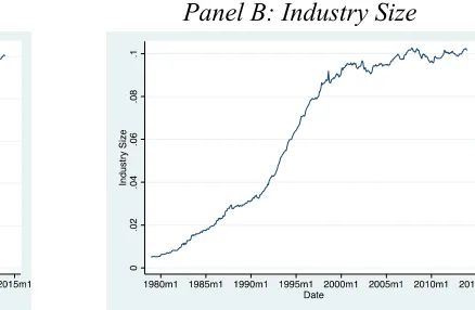
10
mutual funds in the US stock market is shown to increase from below 1% to approximately 10%
of stocks in the past 30 years.
In terms of age variables, FundAge is the length of time since the fund was launched, while
MgrTenure is the length of time since the beginning of the control of the current management.
Although we can easily compute FundAge using the current date and the date when the fund was
launched in CRSP, MgrTenure should be obtained carefully because CRSP does not directly
provide manager tenure data. We use the fund header history data in CRSP to generate
MgrTenure by searching for changes in fund manager information over time. All the changes are
documented to calculate the tenure of each manager.7
4.
Results
4.1
Returns to Scale at Industry Level
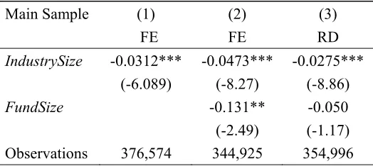
In Table 2, we report the results of decreasing returns to scale on performance at the industry
level, which is consistent with Pástor et al. (2015). In particular, a 1 percentage point increase
in industry size is associated with 0.0312% decrease in monthly performance, which equates to
37 basis points (bps) per year. Note that the 1 percentage point increase in industry size takes
7 Note that some mutual funds are managed by multiple managers. These funds only disclose their management
11
approximately 3.5 years in the sample.
TABLE 2 HERE
If the variable, fund size, is controlled for, we still observe a significantly inverse
relationship between size and performance at the industry level, as shown in Column 2. In
addition, in the FE model, the fund size effect is significantly negative. However, the fund size
effect becomes insignificant when the bias-free RD method is used, as shown in Column 3.8
The decreasing returns to scale at the industry level is consistent with the efficient market
hypothesis. Most mutual funds are institutional investors in the market. The market becomes
increasingly efficient over time as the asset value of the mutual fund increases.
4.2
Threshold Effect on Size-Performance Erosion
Now we consider threshold effects on size-performance erosion. We use two different age
measurement thresholds to investigate the effects of industry size on active mutual fund
performance: MgrTenure and FundAge. These results are reported in Table 3 and Table 4
respectively. Our goal is to investigate if there is any statistical difference of the effects of
industry size on a fund’s performance before and after the thresholds.
8
12 Manager tenure as a threshold
Table 3 reports the results of using manager tenure (i.e. MgrTenure) as a threshold variable for
both the main and the extended samples.
TABLE 3 HERE
Column 1 presents the threshold and the coefficient estimates of gross returns on industry size
without controlling for any variables. Column 2 extends the results by controlling for the fund
size. In Columns 1 and 2 of Panel A, the threshold estimates for manager tenure are close to
1,600 days, approximately 4.4 years. The plot of likelihood ratio is shown in Figure 2. We follow
the method of Hansen (1999) in plotting the likelihood ratio and computing the 95% confidence
interval. On the basis of the asymptotic distribution of threshold estimates, we find the 95%
confidence intervals of [1587, 1603] and [1588, 1604], which are close to the threshold point
estimates for roughly one month.
FIGURE 2 HERE
A fund younger than 4.4 years has smaller decreasing returns to scale of industry size than a
13
and is statistically significant at the 1% level.9 It suggests that young funds suffer less erosion of
performance as a result of increasing industry competition than old funds. Such difference is also
observed in the extended sample, as listed in Panel B of Table 3. Although the scale is different,
the difference between young and old funds remains at 0.01% regardless of the samples and the
presence of control variable, fund size. The estimated threshold is also used to perform the RD
method for fund size, and the results are shown in Column 3. The difference between young and
old funds remains significant despite the insignificant fund size effect.
Fund age as a threshold
Table 4 presents the results of using FundAge as a threshold. In Column 1, the threshold estimate
is 1,608 days (4.4 years), which is close to the value estimated with manager tenure as a
threshold. After controlling for fund size at the same time, the threshold reverts to 1,209 days
(3.3 years), as shown in Column 2. Similar to the case of using manager tenure as a threshold,
changes in industry size cause less performance erosion of young funds (10 to 25 bps) than of
old funds. In Column 1 of Panel A, a young fund shows rising returns to scale of 0.01% per
month, whereas an old fund shows decreasing returns to scale. In Column 2, the difference
between the two coefficients is approximately 0.02. The RD method is applied when fund size is
included, and the results are shown in Column 3. The difference in performance erosion of young
9 See below and Table 5 for our test on the threshold effect. Given that the fund sizes are large on average in the market (with
14
and old funds remains even when using the bias-free method. Similar patterns of difference are
also observed in our extended sample, which is listed in Panel B of Table 4.
TABLE 4 HERE
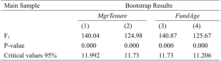
Test for the threshold effect
To show that the threshold effect is statistically significant10, we test the following hypothesis:
H0:12 The likelihood ratio for the test is
F1(S0S1( ˆ)) / ˆ2
.
We do not theoretically derive a standard asymptotic distribution of F1 because the threshold is
endogenously determined; instead, we bootstrap the p-value for the test statistics.11 The results
are presented in Table 5. Columns 1, 2, 3, and 4 show the test results of the regressions in
Columns 1 and 2 of Tables 3 and 4. In all of the threshold model specifications, large F1and
small p-value are found. The null hypothesis is rejected at the 1% significance level. Therefore,
threshold effects of fund age and manager tenure exist in the size-performance relation. In
10
Note that the confidence intervals of the industry size effect on young and old funds overlap in some cases. For example, in Column 2 of Table 3, the confidence intervals for young and old funds are [-0.0492, -0.0266] and [-0.0580, -0.0356] respectively. However, the overlap of confidence interval does not mean there is no statistically significant difference between the groups. It is required to use a further test on the difference of the two groups. 11
15
addition, R-squared notably increases when the threshold model is employed. Although
R-squared remains small in the original FE regression, it increases by at least five times when the
threshold model is used instead.12
TABLE 5 HERE
To summarize, considering both manager tenure and fund age, threshold effects are found in
the relation between industry size and fund performance. For a fund with more than four-year
history, expanding industry size brings a more negative effect on its performance. This
observation suggests that a fund’s performance is likely to worsen as the industry size increases,
particularly when a fund exceeds the age threshold. Therefore, a young fund will experience a
lesser degree of performance erosion compared with an old fund.
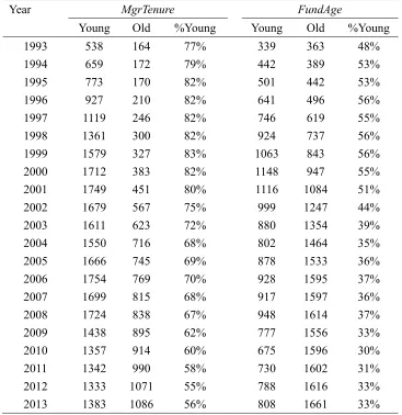
TABLE 6 HERE
We further explore the different results between the two thresholds, MgrTenure and FundAge.
Table 6 presents the statistics of young and old funds, and Figure 3 specifies the proportion of
12
16
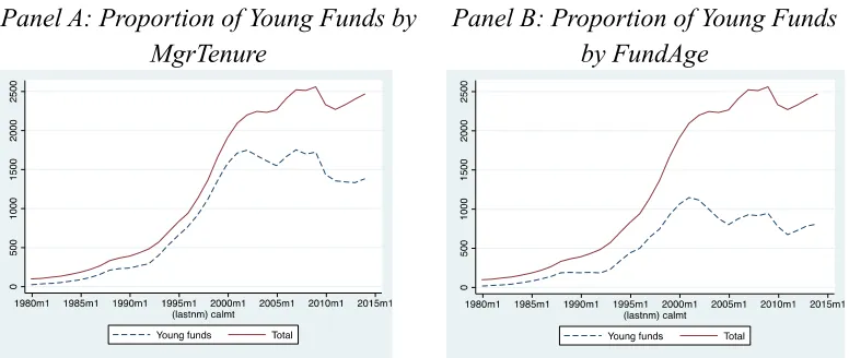
young funds in the industry. Considering the threshold of manager tenure, the percentage of
young funds in the sample decreases from 80% to approximately 55%. Considering the threshold
of fund age, the percentage decreases from 50% to 30%. Figure 3 shows that the proportion of
young funds is declining over time, especially in the 2000s. Therefore, the net entry (entry minus
exit) of mutual funds decreases as the industry develops.
FIGURE 3 HERE TABLE 7 HERE
The estimation results for MgrTenure and FundAge are not completely identical. However,
the threshold estimates are similar, and young funds continue to experience a lesser degree of
performance erosion than old funds. These findings can be explained by the statistics of
MgrTenure and FundAge. The frequencies of changes in fund managers over time are shown in
Table 7. Approximately 50% of the recorded funds have no changes in fund managers. For these
funds, FundAge equals MgrTenure, indicating a partial overlap. Therefore, the threshold
estimates using FundAge and MgrTenure are considerably close.
4.3
Controlling for Other Fund Liquidity Factors
Why do young and old funds differ in terms of returns to scale? To test the hypothesis that
17
and industry levels, we control for liquidity characteristics to examine whether or not the
threshold effect between young and old funds is driven by their difference in liquidity.
We consider three liquidity factors: small-cap fund indicator (I(Sml)), turnover ratio (Turn),
and abnormal return standard error (Std(AbnRet)). Small-cap funds largely invest in small-cap
stocks, thus exerting a large effect on the prices. The turnover ratio measures how actively a fund
allows changes to the portfolio. Abnormal return standard error measures how volatile the active
portfolios are, given that an abnormal return is the return adjusted by a benchmark.
TABLE 8 HERE
Table 8 presents the results of the threshold regression with liquidity factors. The small-cap
fund indicator, turnover ratio, and abnormal return standard error are interacted with the industry
size in our threshold models. First, liquidity constraint still explains the decreasing returns to
scale. In Columns 1, 2, and 3, the liquidity constraint holds because all the coefficients are
negative and significant. This result indicates that funds with lower liquidity tend to suffer a
higher level of decreasing returns to scale. Second, young funds still experience less erosion of
performance than old funds after controlling for liquidity factors. A young small-cap fund suffers
less decreasing returns to scale than an old small-cap fund; the same is true for the turnover ratio
18
consistent results can be obtained when FundAge is used. The difference still holds when the
fund liquidity characteristics are included, indicating that the liquidity difference cannot explain
why the two groups differ.
4.4
Management Skills and Trading Strategies
A possible explanation for the young and old fund difference with respect to the
size-performance is that new entrants can be better equipped. First, young funds might benefit
from talented fund managers with knowledge on new technology. Young funds can have superior
knowledge of stock selection and thus be less affected by increasing competition in the industry.
This is consistent with the findings that the financial industry is packed with highly skilled
financial talents in recent years.13 With relatively sound academic background and better
knowledge of technology, new fund managers are better at identifying financial products that are
undervalued but with good quality.
Second, a young fund needs to have good and stable performance to win the AUM from
incumbents. Wahal and Wang (2011) find that the competition has become fiercer in the US
mutual fund market. Thus, new entrants must possess excellent skills when entering the market
to overtake some of the existing funds. For the sake of reputation, new funds have a high
incentive to outperform others, and an increasing industry size will not result in considerable
19
performance erosion. This situation also explains why new funds have relatively smaller negative
(or even positive) size-performance relationship compared with that of old funds.
To test the aforementioned hypothesis, we implement a trading strategy to compare the
performance of young and old funds. We first classify the funds by young and old portfolios on
the basis of the estimated thresholds of fund age and manager tenure. To construct the portfolios,
we buy young funds and sell old funds. Our estimation is based on lagged values, and hence, at
the beginning of each month, the two portfolios are rebalanced by the fund age or the manager
tenure of the preceding month end. Thereafter, we identify the differences among returns in the
current month and repeat such exercise in the subsequent months to obtain a series of returns.
The gross and adjusted net returns for calculation of the profits of the trading strategy are
computed. Rather than using point estimates, we employ the confidence intervals, and 180 days
before and after the threshold estimates are used to construct broad definitions of the thresholds.
Funds between ages of zero and the lower bound of the thresholds are young funds, whereas
those at ages above the upper bound of the thresholds are old funds.
Pástor et al. (2015) implement similar age-based hypothetical trading strategies to examine
the age-performance relation across funds. However, both young and old funds in the
aforementioned studies are arbitrarily defined according to four age groups, without explicit
evidence namely, 0 to 3, 3 to 6, 6 to 10, and above 10 years. In this paper, we improve the
20
construct the portfolios of young and old funds. Tables 9 and 10 present the results of our trading
strategy based on FundAge and MgrTenure. When FundAge is used, results of Panels A and B in
Table 9 imply that new entrants to the mutual fund industry have superior performance. Returns
are shown in all eight cases; six of these cases are statistically significant at the 5% level, except
the extended sample with the gross return measured for which the positive returns are significant
at the 10% level. In our main sample, the strategy of buying young funds and selling old funds
yields an average of 0.045% monthly gross return and 0.05% monthly net return. These figures
are approximately 0.5% and 0.6% of the annual gross and net returns, respectively, and are both
significant at the 5% level. These results also hold regardless of whether the fees before
measurement (gross return) or fees after measurement (adjusted net return) are used to represent
performance in both our samples.
TABLE 9 HERE TABLE 10 HERE
However, we have different results when using MgrTenure as the threshold. Table 10 shows
that when MgrTenure is used to identify young and old funds and to perform trading strategies,
the differences between young and old funds are statistically insignificant in all cases. The “buy
21
The insignificant result of the MgrTenure trading strategy might be due to the data
limitation of manager tenure and limitations of our treatments in the study. First, fund managers’
years of relevant work experience, which is not available in our sample, would be better
measurements. For example, a fund manager who manages a new fund is likely to have relevant
working experience in the industry. However, such individuals are treated as a brand new
manager in our sample. Second, as documented in Massa et al. (2010), CRSP has noise in the
fund management data, which may affect the accuracy of our calculation. For example, CRSP
treats a fund as having no change of management if the fund is documented as “team-managed”.
A further study on the effects of turnover of management of funds with more accurate data is
necessary to decide whether such change has significant impact on fund performance. Lastly, a
fund manager with either good or bad performance can leave a fund for various reasons.
Therefore, the implementation of the trading strategy based on MgrTenure might not provide
useful insights.
The difference between young and old funds in terms of performance is not the result of
their difference in risk levels. Young funds may hold riskier portfolios to outperform old funds
and succeed by accident. However, Chevalier and Ellison (1999) find that compared with older
managers, younger managers tend to be more conservative and have more conventional
portfolios for job security. The “buy young, sell old” strategy also yields positive returns after the
22
implement the trading strategy, as discussed in Section 4.4. To consider other risk factors, the
Carhart four-factor alpha (Carhart, 1997) is also used to evaluate the returns of the trading
strategy. Table 11 shows that the trading strategy still generates significant positive returns.
TABLE 11 HERE
In conclusion, significant and positive returns are obtained with FundAge as a threshold by
employing the “buy young, sell old” trading strategy. Again, this result is not valid if MgrTenure
is used instead of FundAge.
4.5
Attractiveness of Old Funds
The results presented in Section 4.3 show that young funds outperform old funds and
experience a smaller degree of performance erosion as the industry size grows. Why do people
still prefer old funds and not completely switch to young funds? Table 6 and Figure 3 show that
old funds have been taking up a large percentage in the industry, whereas young funds have
covered a smaller percentage since the 2000s. The number of old funds is also increasing as the
industry size grows. This scenario is contrary to our findings regarding fund performance. Two
explanations are provided. One explanation pertains to risk aversion. Young funds have shorter
track records of their profitability. It would be risky for investors to switch to young funds, even
23
are more likely to invest in old funds. Another explanation is that some institutional investors
may have inertia to fund performance, particularly that of pension plan assets. Several studies
have determined that pension plan assets in mutual funds are sticky and not discerning.14 As
discussed by these studies, pension plan assets in the mutual fund market are sticky and
insensitive to past fund performance. Pension plan participants tend to employ naive investment
strategies; they also rebalance and trade their portfolios infrequently because of their long
horizons and different tax concerns. Consequently, these pension plan participants may hold a
fund for a long period, which may explain why old funds are still popular in the mutual fund
market.
TABLE 12 HERE
To see whether institutional investors take up a large percentage in the mutual fund industry,
Table 12 examines the number of young and old funds across time. Institutional funds aim at
attracting institutional investors, such as pensions, foundations, and endowments. Institutional
funds often have low expenses and loads but require a minimum investment share. In the CRSP
database, the information on whether the fund is institutional only covers the period after 1999;
thus, we summarize the number among young and old funds (with fund age as the threshold)
24
with the available data in the selected year-ends. We classify a fund as “institutional” if one of
the share classes of the fund is documented as an institutional fund in the database. As shown in
Table 12, young funds have a similarly large percentage of institutional funds, although the
number and the percentage are smaller compared with those of old funds.
However, it should be noted that the data only cover the period since 1999; thus, several
data are missing compared with our full sample of funds. In addition, Pan et al. (2014) determine
that institutional funds claimed in fund prospectuses are not ideal measures of institutional
ownership; the researchers find that almost 50% of institutional investors’ holdings are retail
funds. This result suggests that their investment decisions are not based on whether funds are
institutional. Therefore, the results shown in Table 12 may be biased. Further tests are necessary
to verify our explanations.
4.6
Robustness
In this section, we examine the robustness of the threshold effect and the different degrees
of performance erosion of young and old funds. Our results are robust to different samples
after controlling for fund size in the explanatory variables. Section 4 presents the results of
both the main sample (1993–2013) and the extended sample (1979–2013). In both
samples, our threshold estimates and the differences between young and old funds remain
consistent. When fund size is added as an explanatory variable, the threshold estimates and
25
Another concern is incubation bias. Evans (2010) finds that mutual fund families start
multiplying small-size funds privately and only release those with good performance to the
public at the end of an evaluation period. The incubation funds may have inflated performance in
the early stage because they are allowed to use their historical performance as track record. This
scenario makes our inference on the difference between young and old funds biased.
TABLE 13 HERE
To solve the aforementioned problem, observations of funds with sizes smaller than $15
million are excluded during the data learning stage. As a robustness check, the first two years of
records since the funds’ inception are also excluded to examine the threshold estimates and the
difference in parameters, following the methods of Evans (2010). Table 13 shows the results. The
difference between young and old funds in terms of industry size erosion remains robust. Young
funds still have less performance erosion than old funds; the former even have positive returns to
scale. The threshold estimates remain approximately four years; the exception is in Panel B,
Column 1, which notes an increase to five years. The increment is the result of the data trimming
of the first two years. This step considerably reduces the number of observations that lie before
26
remains close to four years. These results suggest that our threshold effects and the difference
between young and old funds are not affected by incubation bias.
5.
Conclusion
In this study, we analyze the nonlinear effect of the decreasing returns to scale of industry size on
mutual fund performance. We apply the threshold model to estimate the effects of industry size
on fund performance in the US mutual fund market. Threshold estimates of critical fund age and
manager tenure are obtained in our sample. This result is in line with those of the studies on
mutual performance persistence. We also acquire evidence that young funds suffer less from
industry size erosion than old funds. Such difference between young and old funds still holds
when fund liquidity characteristics are controlled for. We argue that the difference in the degrees
of performance erosion is caused by the superior features of young funds. This hypothesis is
tested by employing a “buy young, sell old” trading strategy on the basis of our threshold
estimations. This strategy yields significant and positive returns over the years, indicating that
young funds are better equipped than old funds. We also explore the issue of investors’
continuous investment in old funds despite the inferior performance of such funds and explain it
27
References
Benartzi, S., and Thaler, R. H. (2001). Naive diversification strategies in defined contribution saving plans. The American Economic Review, 91(1), 79-98.
Berk, J. B., and Van Binsbergen, J. H. (2015). Measuring skill in the mutual fund industry.
Journal of Financial Economics, 118(1), 1-20.
Berk, J. B., and Green, R. C. (2004). Mutual fund flows and performance in rational markets.
Journal of Political Economy, 112(6), 1269-1295.
Carhart, M. M. (1997). On persistence in mutual fund performance. The Journal of Finance, 52(1), 57-82.
Chen, J., Hong, H., Huang, M., and Kubik, J. D. (2004). Does fund size erode mutual fund performance? The role of liquidity and organization. The American Economic Review, 94(5), 1276-1302.
Chevalier, J., and Ellison, G. (1999). Career concerns of mutual fund managers. The Quarterly Journal of Economics, 114(2), 389-432.
Chong, T. T. L. (2000). Estimating the differencing parameter via the partial autocorrelation function. Journal of Econometrics, 97(2), 365-381.
Chong, T. T. L., Lu, L., and Ongena, S. (2013). Does banking competition alleviate or worsen credit constraints faced by small and medium enterprises? Evidence from China, Journal of Banking and Finance, 37(9), 3412-3424.
Dahlquist, M., and Martinez, J. V. (2015). Investor inattention: A hidden cost of choice in pension plans? European Financial Management, 21(1), 1-19.
Drukker, D., Gomis-Porqueras, P., and Hernandez-Verme, P. (2005). Threshold effects in the relationship between inflation and growth: A new panel-data approach. Working Paper, No. 38225. Munchen: Munich Personal RePEc Archive (MPRA).
Elton, E. J., Gruber, M. J., and Blake, C. R. (2001). A first look at the accuracy of the CRSP mutual fund database and a comparison of the CRSP and Morningstar mutual fund databases.
28
Evans, R. B. (2010). Mutual fund incubation. The Journal of Finance, 65(4), 1581-1611.
Fama, E. F., and French, K. R. (1997). Industry costs of equity. Journal of Financial Economics, 43(2), 153-193.
Hansen, B. E. (1999). Threshold effects in non-dynamic panels: Estimation, testing, and inference. Journal of Econometrics, 93(2), 345-368.
Hjalmarsson, E. (2010). Predicting global stock returns. Journal of Financial and Quantitative
Analysis, 45(1), 49-80.
Massa, M., Reuter, J., and Zitzewitz, E. (2010). When should firms share credit with employees? Evidence from anonymously managed mutual funds. Journal of Financial Economics, 95(3), 400-424.
Pan, X. N., Wang, K., and Zykaj, B. B. (2014). Does institutional ownership predict mutual fund performance? An examination of undiscovered holdings within 13(f) reports. Working paper.
Pástor, Ľ., Stambaugh, R. F., and Taylor, L. A. (2015). Scale and skill in active management.
Journal of Financial Economics, 116(1), 23-45.
Philippon, T., and Reshef, A. (2012). Wages and human capital in the U.S. finance industry: 1909–2006. The Quarterly Journal of Economics, 127(4), 1551-1609.
Reuter, J., and Zitzewitz, E. (2010). How much does size erode mutual fund performance? A regression discontinuity approach. Working paper, No. 16329. Cambridge: National Bureau of Economic Research.
Wahal, S., and Wang, A. Y. (2011). Competition among mutual funds. Journal of Financial
29
Figure 1: Number of Funds and Industry Size
These figures show the change of the US equity active mutual fund market from 1979 to 2013. Panel A shows the number of funds by month since 1979. Panel B shows the industry size, which is the ratio of the sum of assets under management (AUM) of all funds to the aggregate asset value of the stock market.
Panel A: Number of Funds Panel B: Industry Size
Figure 2: Construction of Confidence Interval
These figures show the likelihood ratio of thresholds. Panels A and B use MgrTenure
and FundAge, respectively, as thresholds to construct confidence intervals. We follow the method of Hansen (1999) in plotting the graph and determining the 95% confidence intervals. The horizontal line is used to indicate the confidence interval.
[image:30.612.247.466.174.317.2]30
Figure 3: Proportion of Young Funds
These figures show the proportion of young funds from 1979 to 2013. Young funds are defined as funds that are younger than the threshold estimates. We particularly use 1,600 days for both MgrTenure and FundAge for comparison.
Panel A: Proportion of Young Funds by MgrTenure
31
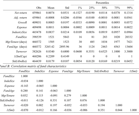
Table 1: Summary Statistics
This table shows the summary statistics. Net return is the monthly net return of management fees and
related operation fees. Adj. return is the net return adjusted for the Fama-French three-factor model.
GrossR is the adjusted return plus expense ratio, which is the monthly expense (i.e., Expense) on fund management and operation. IndustrySize is the ratio of the sum of assets under management of all funds to the aggregate asset value of the US stock market. FundSize is the net asset of a fund at each month end,
adjusted to the dollar rate in December 2013. MgrTenure is the manager tenure, which is calculated by the days elapsed since the current manager took control. FundAge is the age since the start of a fund.
Turnover is the adjusted-to-month turnover of aggregated sales or aggregated purchases of securities divided by the average 12-month total net assets. 1(SmlCap) is used to indicate whether a fund is a small capitalization fund, defined as funds with parameters of small-minus-big factor (Fama-French three-factor
model) over 0.5. Std(AbnRet) is the standard deviation of the adjusted returns (or the alpha of funds) in the Fama-French three-factor model. Correlations between fund characteristics are presented in Panel B.
Panel A: Cross-sectional mean, standard deviation, and percentiles
Percentiles
Obs Mean Std 1% 25% 50% 75% 99%
Net return 459861 0.0074 0.0531 -0.1527 -0.0190 0.0114 0.0378 0.1314
Adj. return 459861 -0.0008 0.0206 -0.0546 -0.0100 -0.0010 0.0081 0.0561
GrossR 409031 0.0003 0.0197 -0.0533 -0.0090 0.0001 0.0093 0.0572
Expense 409498 0.0011 0.0004 0.0002 0.0009 0.0011 0.0014 0.0022
IndustrySize 465478 0.0837 0.0214 0.0109 0.0856 0.0919 0.0957 0.0984
FundSize 398539 1521 5843 16 81 283 1020 20332
MgrTenure(days) 460372 1505 1523 30 485 1034 1977 7421
FundAge (days) 460372 3265.42 2895.96 36 1124 2463 4563 13604
Turnover 382626 0.8340 0.6800 0.0600 0.3551 0.6525 1.1000 3.3800
1(SmlCap) 468206 0.2209 0.4149 0 0 0 0 1
Std(AbnRet) 464439 0.0179 0.0107 0.0054 0.0120 0.0169 0.0219 0.0452
Panel B: Correlation matrix of fund characteristics
FundSize InduSize Expense FundAge MgrTenure Std(AbnRet) Turnover 1(Sml)
FundSize 1.000
InduSize -0.034 1.000
Expense -0.143 -0.065 1.000
FundAge 0.280 0.141 -0.063 1.000
MgrTenure 0.032 0.115 -0.091 0.279 1.000
Std(AbnRet) -0.011 -0.126 0.331 0.107 0.076 1.000
Turnover -0.020 0.002 0.197 -0.052 -0.053 0.194 1.000
32 Table 2: GrossR on Sizes
This table shows the results of GrossR on sizes. IndustrySize is the ratio of the sum of assets under management of all funds to the aggregate asset value of the US stock market. FundSize is the net asset of a fund at each month end, adjusted to the dollar rate in December 2013. RD is the recursive demeaning method proposed by Hjalmarsson (2010). We use the standard error clustered by fund and report the t-statistics in the parentheses. The results on FundSize are multiplied by 106 for enhanced readability.
Main Sample (1) (2) (3)
FE FE RD
IndustrySize -0.0312*** -0.0473*** -0.0275***
(-6.089) (-8.27) (-8.86)
FundSize -0.131** -0.050
(-2.49) (-1.17)
33
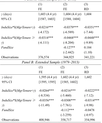
Table 3: Threshold Regressions (MgrTenure)
This table shows the threshold regressions of GrossR on InduSize, with MgrTenure as the threshold. γ is the threshold parameter used to separate young and old funds. We also report the 95% confidence intervals, which are calculated by the likelihood ratio. InduSize is the ratio of the sum of assets under management of all funds to the aggregate asset value of the US stock market. I(MgrTenure < γ) and I(MgrTenure≥γ) are the parameters of young and old funds, respectively.
FundSize is the net asset of a fund at each month end, adjusted to the dollar rate in December 2013. RD is the recursive demeaning method proposed by Hjalmarsson (2010); our estimation treats the thresholds as given in Column 3. We use the standard error clustered by fund and report the t-statistics in the parentheses. The results on FundSize are multiplied by 106 for enhanced readability. We report the results of both the main and the extended samples.
Panel A: Main Sample (1993–2013) (1) FE (2) FE (3) RD γ(days) 95% CI
1,603 (4.4 yr)
[1587, 1603]
1,604 (4.4 yr)
[1588, 1604]
1,604
InduSize*I(MgrTenure<γ) -0.0216*** -0.0379*** -0.0351***
(-4.172) (-6.589) (-7.44)
InduSize*I(MgrTenure≥ γ)
-0.0314*** -0.0468*** -0.0448***
(-6.111) (-8.204) (-9.89)
FundSize -0.127** 0.184
(-2.442) (1.10)
Observations 376,574 344,925 341,221
Panel B: Extended Sample (1979–2013) (1) FE (2) FE (3) RD
γ (days)
95% CI
1,595 (4.4 yr) [1595, 1595]
1,602 (4.4 yr) [1585, 1602]
1,602
InduSize*I(MgrTenure<γ) -0.0264*** -0.0216*** -0.0222*** (-8.534) (-5.460) (-7.12)
InduSize*I(MgrTenure≥ γ)
-0.0356*** -0.0308*** -0.0314***
(-11.49) (-7.761) (-9.98)
FundSize -0.112*** -0.0478
(-3.259) (-0.97)
34
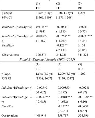
Table 4: Threshold Regressions (FundAge)
This table shows the threshold regressions of GrossR on InduSize, with FundAge as the threshold. γ is the threshold parameter used to separate young and old funds. We also report the 95% confidence intervals calculated by the likelihood ratio. InduSize is the ratio of the sum of assets under management of all funds to the aggregate asset value of the US stock market. I(MgrTenure
< γ) and I(FundAge≥γ) are the parameters of young and old funds, respectively. FundSize is the net asset of a fund at each month end, adjusted to the dollar rate in December 2013. RD is the recursive demeaning method proposed by Hjalmarsson (2010); our estimation treats the thresholds as given in Column 3. We use the standard error clustered by fund and report the t-statistics in the parentheses. The results on FundSize are multiplied by 106 for enhanced readability. We report the results of both the main and the extended samples.
Panel A: Main Sample (1993–2013)
Panel B: Extended Sample (1979–2013) (1) FE (2) FE (3) RD γ (days) 95% CI
1,568 (4.3 yr)
[1568, 1607]
1,209 (3.3 yr)
[1170, 1247]
1,209
InduSize*I(FundAge <γ) -0.00540 0.000850 -0.00285 (-1.482) (0.192) (-0.87)
InduSize*I(FundAge ≥ γ)
-0.0230*** -0.0181*** -0.0190*** (-7.465) (-4.652) (-6.10)
FundSize -1.12*** -0.0430
(-3.331) (-0.87)
Observations 408,946 358,717 354,996
(1) FE (2) FE (3) RD γ (days) 95% CI 1,608 (4.4yr) [1569, 1608] 1,209 (3.3yr) [1171, 1248] 1,209
InduSize*I(FundAge<γ) 0.0115** -0.00843 -0.0043 (1.993) (-1.380) (-0.77)
InduSize*I(FundAge ≥ γ)
-0.00722 -0.0268*** -0.0237***
(-1.389) (-4.769) (-4.84)
FundSize -0.123** 0.174
(-2.430) (-1.05)
35
Table 5: Bootstrap Results
This table shows the bootstrap results for the test on the significance of the threshold effects. Columns 1, 2, 3, and 4 are the test results of the regressions in Columns 1 and 2 of Tables 3 and 4. F1 is the likelihood ratio of the threshold estimates. The p-values are bootstrapped following the
method of Hansen (1999). The critical values are the top 95% quantiles of the likelihood ratio across our bootstrap replications.
Main Sample Bootstrap Results
MgrTenure FundAge
(1) (2) (3) (4)
F1 140.04 124.98 140.87 125.67
P-value 0.000 0.000 0.000 0.000
36
Table 6: Number of Young and Old Funds
This table shows the number of young and old funds from 1993 to 2013. Young funds are defined as funds that are younger than the threshold estimates. We particularly use 1,600 days for both MgrTenure and FundAge for comparison.
Year MgrTenure FundAge
Young Old %Young Young Old %Young
1993 538 164 77% 339 363 48%
1994 659 172 79% 442 389 53%
1995 773 170 82% 501 442 53%
1996 927 210 82% 641 496 56%
1997 1119 246 82% 746 619 55%
1998 1361 300 82% 924 737 56%
1999 1579 327 83% 1063 843 56%
2000 1712 383 82% 1148 947 55%
2001 1749 451 80% 1116 1084 51%
2002 1679 567 75% 999 1247 44%
2003 1611 623 72% 880 1354 39%
2004 1550 716 68% 802 1464 35%
2005 1666 745 69% 878 1533 36%
2006 1754 769 70% 928 1595 37%
2007 1699 815 68% 917 1597 36%
2008 1724 838 67% 948 1614 37%
2009 1438 895 62% 777 1556 33%
2010 1357 914 60% 675 1596 30%
2011 1342 990 58% 730 1602 31%
2012 1333 1071 55% 788 1616 33%
37
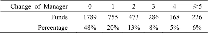
Table 7: Change of Management
This table shows the number of funds based on the number of management changes, the data on which are obtained from the CRSP database.
Change of Manager 0 1 2 3 4 ≥5
Funds 1789 755 473 286 168 226
38
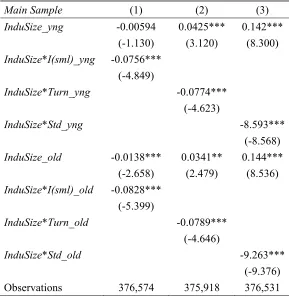
Table 8: Threshold Regression with Liquidity Factors
This table shows the threshold regressions of GrossR on sizes and liquidity factors, with
MgrTenure as the threshold in the main sample. We treat the threshold estimation as given.
IndustrySize is the ratio of the sum of assets under management of all funds to the aggregate asset value of the US stock market. FundSize is the net asset of a fund at each month end, adjusted to the dollar rate in December 2013. The interaction terms are formed by InduSize and
FundSize with I(sml), Turn, and Std, which represent the indicator of small-cap funds, turnover ratio, and standard deviation of abnormal return, respectively. We use “_yng” and “_old” to mark the coefficients of the young and old funds, respectively. We use the standard error clustered by fund and report the t-statistics in the parentheses. The results on FundSize are multiplied by 106 for enhanced readability.
Main Sample (1) (2) (3)
InduSize_yng -0.00594 0.0425*** 0.142*** (-1.130) (3.120) (8.300)
InduSize*I(sml)_yng -0.0756*** (-4.849)
InduSize*Turn_yng -0.0774*** (-4.623)
InduSize*Std_yng -8.593***
(-8.568)
InduSize_old -0.0138*** 0.0341** 0.144*** (-2.658) (2.479) (8.536)
InduSize*I(sml)_old -0.0828*** (-5.399)
InduSize*Turn_old -0.0789*** (-4.646)
InduSize*Std_old -9.263***
(-9.376)
39
Table 9: Trading Strategy (FundAge)
This table shows the result of the “buy young, sell old” trading strategy. At the beginning of each month, we rebalance the two equally weighted portfolios by the fund age of the preceding month end. Thereafter, we obtain the differences in the returns in the current month, repeat this process every month, and compile a series of returns. We use the gross and net returns adjusted with the Fama-French three-factor model for evaluation. We report the means and t-statistics of both portfolios and the difference between the complete strategies, as shown in Columns 1, 2, and 3. The significance level is based on the t-test. We use 180 days before and after the threshold and the confidence interval to provide broad definitions of young and old funds.
Panel A: 180 days before and after the FundAge threshold
Main Sample Younger Funds (%) Older Funds (%) Difference (%)
Gross Return 0.0483 0.00292 0.0453**
(1.28) (0.08) (2.04)
Net Return -0.0569 -0.107*** 0.0502**
(-1.51) (-2.86) (2.22)
Extended Sample Younger Funds (%) Older Funds (%) Difference (%)
Gross Return 0.101*** 0.0578* 0.0427*
(3.09) (1.96) (1.90)
Net Return -0.00692 -0.0489* 0.0419**
(-0.23) (-1.68) (2.15)
Panel B: 95% Confidence interval as the FundAge threshold
Main Sample Younger Funds (%) Older Funds (%) Difference (%)
Gross Return 0.0486 0.00118 0.0473**
(1.30) (0.03) (2.09)
Net Return -0.0572 -0.109*** 0.0515**
(-1.53) (-2.91) (2.24)
Extended Sample Younger Funds (%) Older Funds (%) Difference (%)
Gross Return 0.100*** 0.0568* 0.0435*
(3.08) (1.93) (1.92)
Net Return -0.0064 -0.0497* 0.0432**
40
Table 10: Trading Strategy (MgrTenure)
This table shows the result of the “buy young, sell old” trading strategy. At the beginning of each month, we rebalance the two equally weighted portfolios by the manager tenure of the preceding month end. Thereafter, we obtain the differences in the returns in the current month, repeat this process every month, and compile a series of returns. We use the gross and net returns adjusted with the Fama-French three-factor model for evaluation. We report the means and t-statistics of both portfolios and the difference between the complete strategies, as shown in Columns 1, 2, and 3. The significance level is based on the t-test. We use 180 days before and after the threshold and the confidence interval to provide broad definitions of young and old funds.
Panel A: 180 days before and after the MgrTenure threshold
Main Sample Younger Funds (%) Older Funds (%) Difference (%)
Gross Return 0.0160 0.00194 -0.00348
(0.43) (0.52) (-0.24)
Net Return -0.0915** -0.0894*** -0.00212
(-2.49) (-2.39) (-0.13)
Extended Sample Younger Funds (%) Older Funds (%) Difference (%)
Gross Return 0.0833*** 0.0620** 0.02132
(2.64) (2.115) (1.20)
Net Return -0.0239 -0.0428 0.0200
(-0.81) (-1.52) (1.27)
Panel B: 95% Confidence interval as the MgrTenure threshold
Main Sample Younger Funds (%) Older Funds (%) Difference (%)
Gross Return -0.09242 0.01637 -0.00119
(0.41) (0.44) (-0.089)
Net Return -0.0924** -0.09202** -0.000398
(-2.51) (-2.48) (-0.026)
Extended Sample Younger Funds (%) Older Funds (%) Difference (%)
Gross Return 0.0871** 0.0595** 0.0276
(2.04) (2.03) (1.61)
Net Return -0.00236 -0.0465 0.0229
41
Table 11: Trading Strategy Adjusted for More Risk (FundAge)
This table shows the result of the “buy young, sell old” trading strategy based on FundAge. At the beginning of each month, we rebalance the two equally weighted portfolios by the manager tenure of the preceding month end. Thereafter, we obtain the differences in the returns in the current month, repeat this process every month, and compile a series of returns. We use the returns adjusted with the Carhart four-factor model for evaluation. We report the means and t-statistics of both portfolios and the difference between the complete strategies, as shown in Columns 1, 2, and 3. The significance level is based on the t-test. We use a confidence interval to provide broad definitions of young and old funds.
Main Sample Younger Funds (%) Older Funds (%) Difference (%)
4-Factor Adj. Return -0.61** -0.70** 0.093***
(-2.27) (-2.56) (2.91)
Extended Sample Younger Funds (%) Older Funds (%) Difference (%)
4-Factor Adj. Return -0.59*** -0.67*** 0.075***
42
Table 12: Percentage of Institutional Funds, Selected Years
[image:43.612.86.529.183.299.2]This table shows the number of mutual funds with institutional classes among young funds and old funds in selected years. Young funds and old funds are defined by the threshold estimate in Table 4, with FundAge as the threshold. Institutional funds are documented in the CRSP data set as fund header information.
Year 2000 2005 2006 2007 2008 2009 2010 2011 2012 2013
Old Funds 915 1420 1466 1469 1486 1486 1535 1532 1534 1569
- Institutional Funds 652 1038 1078 1091 1112 1104 1154 1159 1173 1163 Percentage 71% 73% 74% 74% 75% 74% 75% 76% 76% 74%
Young Funds 801 557 554 562 585 579 492 554 564 556
43
Table 13: Robustness Check with First Two Years Removed
This table shows the results of the threshold regressions when we exclude the first two years of observations in the main sample. γ is the threshold parameter used to separate the young and old funds. We also report the 95% confidence intervals, which are calculated by the likelihood ratio.
IndustrySize is the ratio of the sum of assets under management of all funds to the aggregate asset value of the US stock market. InduSize*I(MgrTenure<γ) or InduSize*I(FundAge<γ) is the parameter of the young funds. FundSize is the net asset of a fund at each month end, adjusted to the dollar rate in December 2013. We use the standard error clustered by fund and report the t-statistics in the parentheses. The results on FundSize are multiplied by 106 for enhanced readability.
Panel A: MgrTenure as the threshold (Main Sample)
(1) FE
(2) FE
γ (days)
95% CI
1,603 (4.4 yr)
[1586, 1603]
1,605 (4.4 yr)
[1589, 1605]
InduSize*I(MgrTenure<γ) -0.0193*** -0.0375***
(-3.505) (-6.211)
InduSize*I(MgrTenure≥γ) -0.0281*** -0.0454***
(-5.144) (-7.580)
FundSize -0.123**
(-2.411)
Observations 341,410 313,588
Panel B: FundAge as the threshold (Main Sample)
(1) FE
(2) FE
γ (days)
95% CI
2,006 (5.5 yr)
[2006, 2006]
1,583 (4.3 yr)
[1583, 1989]
InduSize*I(FundAge<γ) 0.0138** -0.00992
(2.327) (-1.544)
InduSize*I(FundAge≥γ) -0.00396 -0.0265*** (-0.727) (-4.470)
FundSize -0.119**
(-2.398)