Proceedings of the 55th Annual Meeting of the Association for Computational Linguistics (Short Papers), pages 372–377 Vancouver, Canada, July 30 - August 4, 2017. c2017 Association for Computational Linguistics
Proceedings of the 55th Annual Meeting of the Association for Computational Linguistics (Short Papers), pages 372–377 Vancouver, Canada, July 30 - August 4, 2017. c2017 Association for Computational Linguistics
A Deep Network with Visual Text Composition Behavior
Hongyu Guo
National Research Council Canada 1200 Montreal Road, Ottawa, Ontario, K1A 0R6
Abstract
While natural languages are composi-tional, how state-of-the-art neural mod-els achieve compositionality is still un-clear. We propose a deep network, which not only achieves competitive accuracy for text classification, but also exhibits com-positional behavior. That is, while creating hierarchical representations of a piece of text, such as a sentence, the lower layers of the network distribute their layer-specific attention weights to individual words. In contrast, the higher layers compose mean-ingful phrases and clauses, whose lengths increase as the networks get deeper until fully composing the sentence.
1 Introduction
Deep neural networks leverage task-specific archi-tectures to develop hierarchical representations of the input, where higher level representations are derived from lower level features (Conneau et al.,
2016). Such hierarchical representations have visually demonstrated compositionality in im-age processing, i.e., pixels combine to form shapes and then contours (Farabet et al., 2013;
Zeiler and Fergus, 2014). Natural languages are
also compositional, i.e., words combine to form phrases and then sentences. Yet unlike in vision, how deep neural models in NLP, which mainly operate on distributed word embeddings, achieve compositionality, is still unclear (Li et al., 2015,
2016).
We propose an Attention Gated Transforma-tion (AGT) network, where each layer’s feature generation is gated by a layer-specific attention mechanism (Bahdanau et al.,2014). Specifically, through distributing its attention to the original given text, each layer of the networks tends to
in-crementallyretrieve new words and phrases from the original text. The new knowledge is then com-bined with the previous layer’s features to create the current layer’s representation, thus resulting in composing longer or new phrases and clauses while creating higher layers’ representations of the text.
Experiments on the Stanford Sentiment Tree-bank (Socher et al., 2013) dataset show that the AGT method not only achieves very competitive accuracy, but also exhibits compositional behav-ior via its layer-specific attention. We empirically show that, given a piece of text, e.g., a sentence, the lower layers of the networks select individ-ual words, e.g, negative and conjunction words
[image:1.595.312.515.568.772.2]not and though, while the higher layers aim at composing meaningful phrases and clauses such as negation phrasenot so much, where the phrase length increases as the networks get deeper until fully composing the whole sentence. Interestingly, after composing the sentence, the compositions of different sentence phrases compete to become the dominating features of the end task.
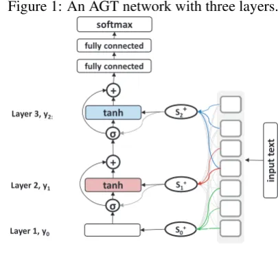
Figure 1: An AGT network with three layers.
S1+
tanh
S2+
tanh
S0+
softmax
σ + fully connected
fully connected
+
σ
input
te
x
t
Layer 1, y0
Layer 2, y1
Layer 3, y2:
2 Attention Gated Transformation Network
Our AGT network was inspired by the Highway Networks (Srivastava et al.,2015a,b), where each layer is equipped with atransform gate.
2.1 Transform Gate for Information Flow
Consider a feedforward neural network with mul-tiple layers. Each layerltypically applies a non-linear transformationf (e.g.,tanh, parameterized by Wfl), on its input, which is the output of the most recent previous layer (i.e.,yl−1), to produce
its outputyl. Here,l = 0indicates the first layer
andy0 is equal to the given input textx, namely
y0 =x:
yl =f(yl−1, Wlf) (1)
While in a highway network (the left column of Figure1), an additional non-linear transform gate functionTlis added to thelth(l >0)layer:
yl=f(yl−1, Wlf)Tl+yl−1(1−Tl) (2)
where the functionTlexpresses how much of the
representationylis produced by transforming the
yl−1 (first term in Equation 2), and how much
is just carrying from yl−1 (second term in
Equa-tion2). HereTlis typically defined as:
Tl=σ(Wltyl−1+btl) (3)
whereWltis the weight matrix andbtlthe bias vec-tor;σis the non-linear activation function.
With transform gateT, the networks learn to de-cide if a feature transformation is needed at each layer. Suppose σ represents a sigmoid function. In such case, the output of T lies between zero and one. Consequently, when the transform gate is one, the networks pass through the transforma-tionf overyl−1and block the pass of inputyl−1;
when the gate is zero, the networks pass through the unmodified yl−1, while the transformation f
overyl−1is suppressed.
The left column of Figure1 reflects the high-way networks as proposed by (Srivastava et al.,
2015b). Our AGT method adds the right two
columns of Figure1. That is, 1) the transform gate
Tlnow is not a function ofyl−1, but a function of
the selection vectors+l , which is determined by the attention distributed to the given inputxby thelth
layer (will be discussed next), and 2) the function
f takes as input the concatenation ofyl−1 ands+l
to create feature representationyl. These changes
result in an attention gated transformation when forming hierarchical representations of the text.
2.2 Attention Gated Transformation
In AGT, the activation of the transform gate at each layer depends on a layer-specific attention mecha-nism. Formally, given a piece of textx, such as a sentence withN words, it can be represented as a matrixB∈IRN×d. Each row of the matrix corre-sponds to one word, which is represented by ad -dimensional vector as provided by a learned word embedding table. Consequently, the selection vec-tor s+l , for thelth layer, is the softmax weighted sum over theN word vectors inB:
s+l =
N
X
n=1
dl,nB[n:n] (4)
with the weight (i.e., attention)dl,ncomputed as:
dl,n=
exp(ml,n)
PN
n=1exp(ml,n)
(5)
ml,n=wml tanh(Wlm(B[n:n])) (6)
here, wml and Wlm are the weight vector and weight matrix, respectively. By varying the at-tention weightdl,n, thes+l can focus on different
rows of the matrix B, namely different words of the given text x, as illustrated by different color curves connecting to s+ in Figure 1. Intuitively, one can consider s+ as a learned word selection component: choosing different sets of words of the given textxby distributing its distinct attention.
Having built one s+ for each layer from the given textx, the activation of the transform gate for layerl(l >0)(i.e., Equation3) is calculated:
Tl=σ(Wlts+l +btl) (7)
To generate feature representationyl, the function
f takes as input the concatenation ofyl−1ands+l .
That is, Equation2becomes:
yl=
(
s+l , l= 0
f([yl−1;s+l ], Wlf)Tl+yl−1(1−Tl), l >0
(8)
where [...;...] denotes concatenation. Thus, at each layerl, the gateTl can regulate either
knowledge from the input textxto augmentyl−1
to create a better representation foryl.
Finally, as depicted in Figure1, the feature rep-resentation of the last layer of the AGT is fed into two fully connected layers followed by a softmax function to produce a distribution over the possi-ble target classes. For training, we use multi-class cross entropy loss.
Note that, Equation8 indicates that the repre-sentationyldepends on boths+l andyl−1. In other
words, although Equation7states that the gate ac-tivation at layerlis computed bys+l , the gate acti-vation is also affected byyl−1, which embeds the
information from the layers belowl.
Intuitively, the AGT networks are encouraged to consider new words/phrases from the input text at higher layers. Consider the fact that the s+0 at the bottom layer of the AGT only deploys a lin-ear transformation of the bag-of-words features. If no new words are used at higher layers of the networks, it will be challenge for the AGT to sufficiently explore different combinations of word sets of the given text, which may be im-portant for building an accurate classifier. In con-trast, through tailoring its attention for new words at different layers, the AGT enables the words selected by a layer to be effectively combined with words/phrases selected by its previous lay-ers to benefit the accuracy of the classification task (more discussions are presented in Section3.2).
3 Experimental Studies
3.1 Main Results
The Stanford Sentiment Treebank data contains 11,855 movie reviews (Socher et al., 2013). We use the same splits for training, dev, and test data as in (Kim, 2014) to predict the fine-grained 5-class sentiment categories of the sen-tences. For comparison purposes, following (Kim,
2014;Kalchbrenner et al.,2014;Lei et al.,2015),
we trained the models using both phrases and sentences, but only evaluate sentences at test time. Also, we initialized all of the word em-beddings (Cherry and Guo, 2015;Chen and Guo,
2015) using the 300 dimensional pre-trained vec-tors from GloVe (Pennington et al., 2014). We learned 15 layers with 200 dimensions each, which requires us to project the 300 dimensional word vectors; we implemented this using a lin-ear transformation, whose weight matrix and bias term are shared across all words, followed by
a tanh activation. For optimization, we used Adadelta (Zeiler, 2012), with learning rate of 0.0005, mini-batch of 50, transform gate bias of 1, and dropout (Srivastava et al., 2014) rate of 0.2. All these hyperparameters were determined through experiments on the validation-set.
AGT 50.5
high-order CNN 51.2
tree-LSTM 51.0
DRNN 49.8
PVEC 48.7
DCNN 48.5
DAN 48.2
CNN-MC 47.4
CNN 47.2
RNTN 45.7
NBoW 44.5
RNN 43.2
[image:3.595.360.474.152.287.2]SVM 38.3
Table 1: Test-set accuracies obtained; results ex-cept the AGT are drawn from (Lei et al.,2015).
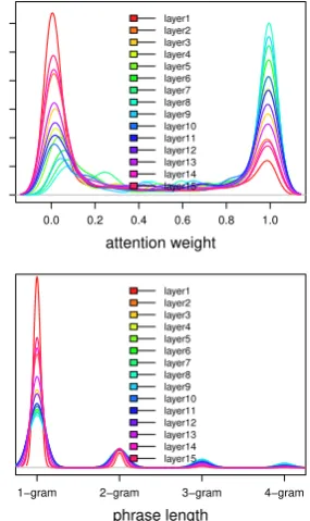
Figure 2: Soft attention distribution (top) and phrase length distribution (bottom) on the test set.
0.0 0.2 0.4 0.6 0.8 1.0
0
1
2
3
4
5
6
attention weight
layer1 layer2 layer3 layer4 layer5 layer6 layer7 layer8 layer9 layer10 layer11 layer12 layer13 layer14 layer15
phrase length
1−gram 2−gram 3−gram 4−gram
layer1 layer2 layer3 layer4 layer5 layer6 layer7 layer8 layer9 layer10 layer11 layer12 layer13 layer14 layer15
Table1presents the test-set accuracies obtained by different strategies. Results in Table 1 indi-cate that the AGT method achieved very competi-tive accuracy (with 50.5%), when compared to the state-of-the-art results obtained by the tree-LSTM (51.0%) (Tai et al., 2015; Zhu et al., 2015) and high-order CNN approaches (51.2%) (Lei et al.,
2015).
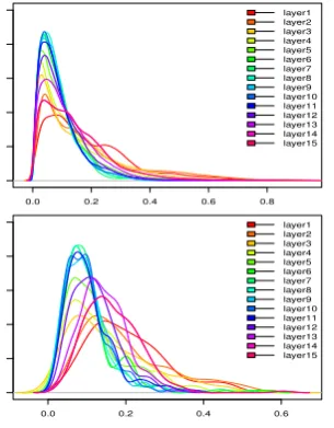
[image:3.595.341.484.383.623.2]distribu-Figure 3: Transform gate activities of the test-set (top) and the first sentence in Figure4(bottom).
0.0 0.2 0.4 0.6 0.8
0
2
4
6
8
10 layer1
layer2 layer3 layer4 layer5 layer6 layer7 layer8 layer9 layer10 layer11 layer12 layer13 layer14 layer15
0.0 0.2 0.4 0.6
0
2
4
6
8
10 layer1
layer2 layer3 layer4 layer5 layer6 layer7 layer8 layer9 layer10 layer11 layer12 layer13 layer14 layer15
tions of the attention weights created by differ-ent layers on all test data, where the attdiffer-ention weights of all words in a sentence, i.e., dl,n in
Equation 4, are normalized to the range between 0 and 1 within the sentence. The figure indicates that AGT generated very spiky attention distribu-tion. That is, most of the attention weights are ei-ther 1 or 0. Based on these narrow, peaked bell curves formed by the normal distributions for the attention weights of 1 and 0, we here consider a word has been selectedby the networks if its at-tention weight is larger than 0.95, i.e., receiving more than 95% of the full attention, and a phrase has beencomposed and selectedif a set of consec-utive words all have been selected.
In the bottom subfigure of Figure2we present the distribution of the phrase lengths on the test set. This figure indicates that the middle layers of the networks e.g., 8thand 9th, have longer phrases (green and blue curves) than others, while the lay-ers at the two ends contain shorter phrases (red and pink curves).
In Figure 3, we also presented the transform gate activities on all test sentences (top) and that of the first example sentence in Figure4(bottom). These curves suggest that the transform gates at the middle layers (green and blue curves) tended to be close to zero, indicating the pass-through of lower layers’ representations. On the contrary, the gates at the two ends (red and pink curves) tended to be away from zero with large tails, implying the retrieval of new knowledge from the input text. These are consistent with the results below.
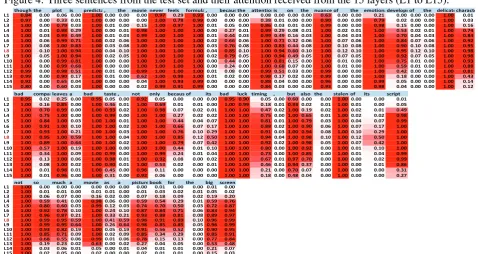
Figure 4 presents three sentences with various lengths from the test set, with the attention weights numbered and then highlighted in heat map. Fig-ure4suggests that the lower layers of the networks selected individual words, while the higher layers aimed at phrases. For example, the first and sec-ond layers seem toselect individual words carry-ing strong sentiment (e.g.,predictable,bad,never
anddelicate), and conjunction and negation words
(e.g., though andnot). Also, meaningful phrases werecomposed and selectedby later layers, such
asnot so much,not only... but also,bad taste,bad
luck, emotional development, and big screen. In
addition, in the middle layer, i.e., the 8th layer, the whole sentences were composed by filtering out uninformative words, resulting in concise ver-sions, as follows (selected words and phrases are highlighted in color blocks).
1)though plotpredictablemovie never
feels formulaic attention nuances
emo-tional developmentdelicate characters
2) bad company leaves bad taste not
onlybad luckbut alsostalenessscript
3)not so muchmoviepicturebig screen
Interestingly, if relaxing the word selection cri-teria, e.g., including words receiving more than the median, rather than 95%, of the full attention, the sentences recruited more conjunction and modifi-cation words, e.g.,because,for,a,itsandon, thus becoming more readable and fluent:
1)thoughplot is predictablemovie never
feels formulaic because attention is on
nuancesemotional developmentdelicate
characters
2)bad company leaves a bad taste not
only becauseits bad luck timingbut also
stalenessits script
3)not so much a movie a picture book
forbig screen
Now, consider the AGT’s compositional behavior for a specific sentence, e.g., the last sentence in Figure4. The first layer solelyselectedthe word
not(with attention weight of 1 and all other words with weights close to 0), but the 2nd to 4th lay-ers gradually pulled out new wordsbook, screen
and movie from the given text. Incrementally,
the 5th and 6th layers further selected words to form phrases not so much, picture book, and big
[image:4.595.103.256.100.296.2]Figure 4: Three sentences from the test set and their attention received from the 15 layers (L1 to L15).
though the plot is predicta , the movie never feels formula , becaus the attentionis on the nuance of the emotionadevelopmof the delicatecharacte L1 0.84 0.00 0.06 0.00 1.00 0.00 0.00 0.00 0.97 0.29 0.93 0.00 0.00 0.00 0.08 0.00 0.00 0.00 0.63 0.00 0.00 0.21 0.00 0.00 0.00 1.00 0.01 L2 0.97 0.00 0.33 0.01 1.00 0.00 0.00 0.00 1.00 0.78 0.99 0.00 0.00 0.00 0.38 0.01 0.00 0.00 0.90 0.00 0.00 0.79 0.02 0.00 0.00 1.00 0.03 L3 1.00 0.00 0.79 0.03 1.00 0.01 0.00 0.15 1.00 0.97 1.00 0.01 0.05 0.00 0.86 0.03 0.01 0.00 0.99 0.00 0.00 0.98 0.15 0.00 0.00 1.00 0.16 L4 1.00 0.01 0.98 0.29 1.00 0.00 0.01 0.98 1.00 1.00 1.00 0.00 0.27 0.01 0.99 0.29 0.08 0.01 1.00 0.02 0.01 1.00 0.53 0.02 0.01 1.00 0.74 L5 1.00 0.03 0.99 0.49 1.00 0.01 0.03 0.99 1.00 1.00 1.00 0.01 0.44 0.03 0.99 0.49 0.16 0.03 1.00 0.04 0.03 1.00 0.70 0.04 0.03 1.00 0.84 L6 1.00 0.06 0.99 0.71 1.00 0.02 0.06 1.00 1.00 1.00 1.00 0.02 0.66 0.06 1.00 0.71 0.32 0.06 1.00 0.07 0.06 1.00 0.84 0.07 0.06 1.00 0.92 L7 1.00 0.08 1.00 0.83 1.00 0.03 0.08 1.00 1.00 1.00 1.00 0.03 0.76 0.08 1.00 0.83 0.44 0.08 1.00 0.10 0.08 1.00 0.90 0.10 0.08 1.00 0.95
L8 1.00 0.10 1.00 0.94 1.00 0.04 0.10 1.00 1.00 1.00 1.00 0.04 0.85 0.10 1.00 0.94 0.60 0.10 1.00 0.12 0.10 1.00 0.95 0.12 0.10 1.00 0.98 L9 1.00 0.05 1.00 0.94 1.00 0.02 0.05 1.00 1.00 1.00 1.00 0.02 0.79 0.05 1.00 0.94 0.49 0.05 1.00 0.07 0.05 1.00 0.92 0.07 0.05 1.00 0.98 L10 1.00 0.00 0.99 0.81 1.00 0.00 0.00 1.00 1.00 1.00 1.00 0.00 0.44 0.00 1.00 0.81 0.15 0.00 1.00 0.01 0.00 1.00 0.75 0.01 0.00 1.00 0.93 L11 1.00 0.00 0.99 0.68 1.00 0.00 0.00 1.00 1.00 1.00 1.00 0.00 0.24 0.00 1.00 0.68 0.07 0.00 1.00 0.01 0.00 1.00 0.59 0.01 0.00 1.00 0.88 L12 0.99 0.00 0.98 0.51 1.00 0.01 0.00 0.99 1.00 1.00 1.00 0.01 0.08 0.00 0.99 0.51 0.03 0.00 0.99 0.00 0.00 1.00 0.42 0.00 0.00 1.00 0.81 L13 0.99 0.00 0.90 0.17 1.00 0.01 0.00 0.62 1.00 0.98 1.00 0.01 0.02 0.00 0.98 0.17 0.02 0.00 0.99 0.00 0.00 1.00 0.18 0.00 0.00 1.00 0.43 L14 0.92 0.00 0.65 0.04 1.00 0.00 0.00 0.04 1.00 0.93 0.99 0.00 0.00 0.00 0.88 0.04 0.00 0.00 0.96 0.00 0.00 0.99 0.05 0.00 0.00 1.00 0.14 L15 0.80 0.00 0.60 0.03 1.00 0.00 0.00 0.02 0.99 0.91 0.99 0.00 0.00 0.00 0.84 0.03 0.00 0.00 0.93 0.00 0.00 0.98 0.04 0.00 0.00 1.00 0.12
bad companleaves a bad taste , not only becaus of its bad luck timing , but also the staleneof its script L1 0.95 0.02 0.25 0.00 0.95 0.05 0.00 0.92 0.05 0.00 0.00 0.00 0.95 0.90 0.05 0.00 0.60 0.00 0.00 1.00 0.00 0.00 0.01 L2 1.00 0.16 0.85 0.00 1.00 0.46 0.01 1.00 0.69 0.01 0.01 0.00 1.00 0.99 0.18 0.01 0.93 0.02 0.01 1.00 0.01 0.00 0.05 L3 1.00 0.70 0.99 0.00 1.00 0.93 0.02 1.00 0.98 0.07 0.02 0.01 1.00 1.00 0.47 0.02 1.00 0.19 0.02 1.00 0.02 0.01 0.49 L4 1.00 0.75 1.00 0.00 1.00 0.99 0.00 1.00 1.00 0.27 0.02 0.02 1.00 1.00 0.75 0.00 1.00 0.65 0.01 1.00 0.02 0.02 0.98 L5 1.00 0.84 1.00 0.03 1.00 1.00 0.01 1.00 1.00 0.44 0.04 0.07 1.00 1.00 0.81 0.01 1.00 0.79 0.03 1.00 0.04 0.07 0.99 L6 1.00 0.91 1.00 0.10 1.00 1.00 0.02 1.00 1.00 0.66 0.07 0.17 1.00 1.00 0.88 0.02 1.00 0.90 0.06 1.00 0.07 0.17 1.00 L7 1.00 0.93 1.00 0.21 1.00 1.00 0.03 1.00 1.00 0.76 0.10 0.29 1.00 1.00 0.91 0.03 1.00 0.94 0.08 1.00 0.10 0.29 1.00
L8 1.00 0.95 1.00 0.59 1.00 1.00 0.04 1.00 1.00 0.85 0.12 0.50 1.00 1.00 0.94 0.04 1.00 0.98 0.10 1.00 0.12 0.50 1.00 L9 1.00 0.89 1.00 0.64 1.00 1.00 0.02 1.00 1.00 0.79 0.07 0.42 1.00 1.00 0.92 0.02 1.00 0.98 0.05 1.00 0.07 0.42 1.00 L10 1.00 0.57 1.00 0.19 1.00 1.00 0.00 1.00 1.00 0.44 0.01 0.10 1.00 1.00 0.80 0.00 1.00 0.92 0.00 1.00 0.01 0.10 1.00 L11 1.00 0.34 1.00 0.09 1.00 0.99 0.00 1.00 0.99 0.24 0.01 0.04 1.00 1.00 0.73 0.00 1.00 0.85 0.00 1.00 0.01 0.04 0.99 L12 1.00 0.13 1.00 0.06 1.00 0.98 0.01 1.00 0.92 0.08 0.00 0.02 1.00 1.00 0.67 0.01 0.97 0.70 0.00 1.00 0.00 0.02 0.99 L13 1.00 0.08 1.00 0.02 1.00 0.90 0.01 1.00 0.53 0.02 0.00 0.01 1.00 1.00 0.46 0.01 0.94 0.37 0.00 1.00 0.00 0.01 0.86 L14 1.00 0.01 0.98 0.01 1.00 0.45 0.00 0.96 0.11 0.00 0.00 0.00 1.00 1.00 0.21 0.00 0.70 0.07 0.00 1.00 0.00 0.00 0.31 L15 1.00 0.01 0.96 0.00 1.00 0.31 0.00 0.92 0.06 0.00 0.00 0.00 1.00 1.00 0.18 0.00 0.48 0.04 0.00 1.00 0.00 0.00 0.27
not so much a movie as a picture book for the big screen L1 1.00 0.00 0.00 0.00 0.00 0.00 0.00 0.00 0.01 0.00 0.00 0.01 0.00 L2 1.00 0.01 0.01 0.00 0.01 0.01 0.00 0.01 0.03 0.02 0.01 0.05 0.02 L3 1.00 0.06 0.07 0.00 0.16 0.02 0.00 0.07 0.18 0.09 0.02 0.19 0.20 L4 1.00 0.59 0.41 0.00 0.98 0.06 0.00 0.59 0.54 0.29 0.01 0.59 0.76 L5 1.00 0.80 0.60 0.03 0.99 0.12 0.03 0.74 0.70 0.50 0.03 0.72 0.87 L6 1.00 0.92 0.78 0.10 1.00 0.24 0.10 0.87 0.84 0.71 0.06 0.83 0.94 L7 1.00 0.96 0.87 0.21 1.00 0.33 0.21 0.93 0.88 0.81 0.08 0.89 0.97
L8 1.00 0.99 0.95 0.59 1.00 0.41 0.59 0.98 0.91 0.89 0.10 0.96 0.99 L9 1.00 0.99 0.95 0.64 1.00 0.26 0.64 0.98 0.85 0.85 0.05 0.96 0.99 L10 1.00 0.93 0.82 0.19 1.00 0.05 0.19 0.91 0.56 0.52 0.00 0.90 0.95 L11 1.00 0.85 0.71 0.09 1.00 0.02 0.09 0.85 0.34 0.29 0.00 0.85 0.91 L12 1.00 0.68 0.55 0.06 0.99 0.01 0.06 0.78 0.15 0.13 0.00 0.77 0.84 L13 1.00 0.19 0.23 0.02 0.63 0.00 0.02 0.27 0.04 0.05 0.00 0.53 0.48 L14 1.00 0.03 0.06 0.01 0.05 0.00 0.01 0.04 0.01 0.01 0.00 0.21 0.07 L15 1.00 0.02 0.05 0.00 0.02 0.00 0.00 0.02 0.01 0.01 0.00 0.15 0.03
conjunction and quantification wordsaandforto make the sentence more fluent. This recursive composing process resulted in the sentence “not
so much a movie a picture book for big screen”.
Interestingly, Figures4 and 2 also imply that, after composing the sentences by the middle layer, the AGT networks shifted to re-focus on shorter phrases and informative words. Our analysis on the transform gate activities suggests that, dur-ing this re-focusdur-ing stage the compositions of sen-tence phrases competed to each others, as well as to the whole sentence composition, for the domi-nating task-specific features to represent the text.
3.2 Further Observations
As discussed at the end of Section2.2, intuitively, including new words at different layers allows the networks to more effectively explore different combinations of word sets of the given text than that of using all words only at the bottom layer of the networks. Empirically, we observed that, if with onlys+0 in the AGT network, namely remov-ing s+i for i > 0, the test-set accuracy dropped from 50.5% to 48.5%. In other words, transform-ing a linear combination of the bag-of-words fea-tures was insufficient for obtaining sufficient ac-curacy for the classification task. For instance, if being augmented with two more selection vectors
s+i , namely removings+i fori >2, the AGT was
able to improve its accuracy to 49.0%.
Also, we observed that the AGT networks tended to select informative words at the lower layers. This may be caused by the recursive form of Equation 8, which suggests that the words re-trieved bys+0 have more chance to combine with and influence the selection of other feature words. In our study, we found that, for example, the top 3 most frequent words selected by the first layer of the AGT networks were all negation words:n’t, never, andnot. These are important words for sen-timent classification (Zhu et al.,2014).
In addition, like the transform gate in the High-way networks (Srivastava et al., 2015a) and the forget gate in the LSTM (Gers et al., 2000), the attention-based transform gate in the AGT net-works is sensitive to its bias initialization. We found that initializing the bias to one encouraged the compositional behavior of the AGT networks.
4 Conclusion and Future Work
References
Dzmitry Bahdanau, Kyunghyun Cho, and Yoshua
Ben-gio. 2014. Neural machine translation by jointly
learning to align and translate. InICLR 2015.
Boxing Chen and Hongyu Guo. 2015. Representation
based translation evaluation metrics. InACL (2).
pages 150–155.
Colin Cherry and Hongyu Guo. 2015. The unreason-able effectiveness of word representations for
twit-ter named entity recognition. InHLT-NAACL. pages
735–745.
Alexis Conneau, Holger Schwenk, Lo¨ıc Barrault, and Yann LeCun. 2016. Very deep convolutional
net-works for natural language processing. CoRR
abs/1606.01781.
Cl´ement Farabet, Camille Couprie, Laurent Najman, and Yann LeCun. 2013. Learning hierarchical
fea-tures for scene labeling. IEEE Trans. Pattern Anal.
Mach. Intell.35(8):1915–1929.
Felix A. Gers, J¨urgen A. Schmidhuber, and Fred A. Cummins. 2000. Learning to forget: Continual
pre-diction with lstm. Neural Comput. 12(10):2451–
2471.
Hongyu Guo. 2015. Generating text with deep
rein-forcement learning. InNIPS2015 Deep
Reinforce-ment Learning Workshop.
Zhiting Hu, Zichao Yang, Xiaodan Liang, Ruslan Salakhutdinov, and Eric P Xing. 2017. Controllable
text generation.arXiv preprint arXiv:1703.00955.
Nal Kalchbrenner, Edward Grefenstette, and Phil
Blun-som. 2014. A convolutional neural network for
modelling sentences.CoRRabs/1404.2188.
Yoon Kim. 2014. Convolutional neural networks for
sentence classification.CoRRabs/1408.5882.
Tao Lei, Regina Barzilay, and Tommi S. Jaakkola.
2015. Molding cnns for text: linear,
non-consecutive convolutions.CoRRabs/1508.04112.
Jiwei Li, Xinlei Chen, Eduard H. Hovy, and Dan Ju-rafsky. 2015. Visualizing and understanding neural
models in NLP.CoRRabs/1506.01066.
Jiwei Li, Will Monroe, and Dan Jurafsky. 2016. Un-derstanding neural networks through representation
erasure.arXiv preprint arXiv:1612.08220.
Jeffrey Pennington, Richard Socher, and Christopher D Manning. 2014. Glove: Global vectors for word
representation. InEMNLP. volume 14, pages 1532–
43.
Richard Socher, Alex Perelygin, Jean Y. Wu, Jason Chuang, Christopher D. Manning, Andrew Y. Ng, and Christopher Potts. 2013. Recursive deep mod-els for semantic compositionality over a sentiment
treebank. InEMNLP ’13.
Nitish Srivastava, Geoffrey Hinton, Alex Krizhevsky, Ilya Sutskever, and Ruslan Salakhutdinov. 2014. Dropout: A simple way to prevent neural networks
from overfitting. J. Mach. Learn. Res.15(1).
Rupesh Kumar Srivastava, Klaus Greff, and J¨urgen
Schmidhuber. 2015a. Highway networks. CoRR
abs/1505.00387.
Rupesh Kumar Srivastava, Klaus Greff, and J¨urgen Schmidhuber. 2015b. Training very deep networks. In Proceedings of the 28th International Confer-ence on Neural Information Processing Systems. NIPS’15, pages 2377–2385.
Kai Sheng Tai, Richard Socher, and Christopher D. Manning. 2015. Improved semantic representations from tree-structured long short-term memory
net-works. CoRRabs/1503.00075.
Matthew D. Zeiler. 2012. ADADELTA: an adaptive
learning rate method. CoRRabs/1212.5701.
Matthew D. Zeiler and Rob Fergus. 2014. Visualizing
and understanding convolutional networks. In
Com-puter Vision - ECCV 2014 - 13th European Con-ference, Zurich, Switzerland, September 6-12, 2014, Proceedings, Part I. pages 818–833.
Xiaodan Zhu, Hongyu Guo, Saif Mohammad, and Svetlana Kiritchenko. 2014. An empirical study on
the effect of negation words on sentiment. In ACL
(1). pages 304–313.
Xiaodan Zhu, Parinaz Sobhani, and Hongyu Guo.
2015. Long short-term memory over recursive