Munich Personal RePEc Archive
People do not adapt to income changes:
A re-evaluation of the dynamic effects of
(reference) income on life satisfaction
with GSOEP and UKHLS data
Kaiser, Caspar
Nuffield College, Oxford, Department of Social Policy and
Intervention
2 November 2018
People do not adapt to income changes:
A re-evaluation of the dynamic effects of (reference) income on
life satisfaction with GSOEP and UKHLS data
∗
Caspar Kaiser
†Department of Social Policy and Intervention
and
Nuffield College, University of Oxford
November 2018
Abstract
Do people adapt to changes in income? This paper shows that there is no evidence of adaptation to income in GSOEP (1984-2015) and UKHLS (1996-2015) data. Following the empirical approach of
Vendrik(2013), I arrive at this surprising answer by estimating (dynamic) life satisfaction equations, in which I simultaneously enter contemporaneous and lagged terms for a respondent’s own house-hold income and their estimated reference income. Additionally, I instrument for own income and include lags of a large set of controls. Furthermore, I find that people also do not adapt to changes in reference income. Instead, reference income effects may be subject to reinforcement over time. To explain my findings, a comprehensive account of the puzzling and often divergent results ofFerrer-i Carbonell and Van Praag(2008),Binder and Coad(2010),Di Tella et al.(2010), andPfaff(2013) is given. What was found to be adaptation to raw household income in these studies turns out to have been driven by reinforcement of an initially small negative effect of household size that grows large over time. Implications of this result for the estimation of equivalence scales with subjective data are discussed.
Keywords: subjective well-being, life satisfaction, adaptation, income comparisons, equivalence scales, GSOEP, BHPS, Understanding Society, UKHLS
JEL codes: D6, I31
∗I thank Anders Bach-Mortensen, Andrew Oswald, Karl Overdick, Mariano Rojas, Nhat An Trinh, as well as participants of the Oxford DSPI Poverty and Inequality Research Groups for helpful comments on an earlier draft. I especially thank Brian Nolan and Maarten Vendrik for their extensive and insightful comments and suggestions. Funding from Nuffield College (Oxford) and the Department of Social Policy and Intervention (Oxford) is gratefully acknowledged.
1
Introduction
When people earn more, they tend to become more satisfied with their lives. However, with time, people may grow accustomed to higher incomes. As a consequence, people’s life satisfaction tends to decline. This phenomenon is commonly called adaptation. In the present study, I show thatnosignificant adaptation to income can be observed in two of the data-sets (GSOEP and UKHLS1
) that are most commonly used in the study of happiness.
With this paper I follow a large literature that evaluates whether people adapt to various life events more generally (for studies on adaptation in non-pecuniary domains, see e.g. Angeles,2010;Clark et al., 2008; Hanglberger and Merz,2011). There are some previous studies that investigate whether we adapt to income in life satisfaction (e.g. Di Tella et al.,2010; Di Tella and MacCulloch,2010; Vendrik,2013; Ferrer-i Carbonell and Van Praag, 2008; Wolbring et al., 2013). However, those studies do not form a consensus. Despite this lack of consensus, a number of authors, particularly those working in the capabilities approach, simply assume that adaptation to income in life satisfaction has been empirically established (Sen,1985;Nussbaum,2000;Qizilbash,2006;Schokkaert,2007;Jayawickreme and Pawelski, 2012;Graham and Nikolova,2015) - a presumed fact which can then be used to undermine the normative significance that may be put upon measures of life satisfaction. Furthermore, adaptation has previously been put forward as a possible explanation for the well-known and much debated Easterlin Paradox (Clark et al.,2008; Clark,2015; Easterlin, 2016). Thus, there is some importance to assessing whether adaptation to income in life satisfaction does in fact occur.
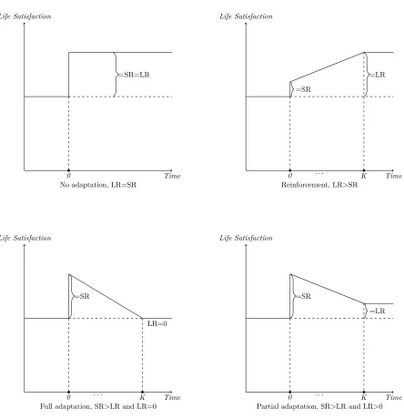
Before doing so, it is useful to clarify my terminology. By adaptation to income I mean that the absolute size of the long-run2
effect of income on life satisfaction is smaller than the absolute size of the contemporaneous effect of income on life satisfaction. One may further distinguish between partial and full adaptation. Partial adaptation refers to a situation in which the absolute size of the long-run effect is indeed smaller, but where the long-run effect is nevertheless significant and of the same sign. In contrast, full adaptation occurs in situations where the contemporaneous effect is significant, but the long-run effect is zero, or insignificant. Following Vendrik(2013), I call the opposite of adaptation “reinforcement”. Reinforcement occurs when long- and short-run effects have the same sign and when the absolute size of the long-run effect of income on life satisfaction is larger than the absolute size of the short-run effect3
. An illustration of reinforcement, as well as full and partial adaptation is given in figure1.
In almost all studies (exceptVendrik,2013), adaptation to income is exclusively taken to be adaptation toownincome. However, this need not be so. Given that we know that the incomes of peers (henceforth, “reference incomes”) tend to have negative contemporaneous effects on life satisfaction (e.g. McBride, 2001; Ferrer-i Carbonell,2005; Vendrik and Woltjer, 2007), it may well be that such reference incomes could also be subject to either adaptation or reinforcement. If so, it then becomes useful to evaluate what the dynamic effect of joint income, i.e. the combined effect of own and reference income is. Doing so is particularly important, since only observing a nil or negative long-run effect of joint income would be compatible with the postulate of the Easterlin Paradox that the long-run time-series correlation of
1Which is a combination of the older British Household Panel Study (BHPS) and its successor Understanding Society. 2I take the long-run to be a situation in which income and life satisfaction are unchanging and in equilibrium with respect to each other.
Life Satisfaction
Time
=SR=LR
0
No adaptation, LR=SR
Life Satisfaction
Time
=SR
=LR
0 . . . K
Reinforcement, LR>SR
Life Satisfaction
Time
=SR
LR=0
0 . . . K
Full adaptation, SR>LR and LR=0
Life Satisfaction
Time
=SR
=LR
0 . . . K
[image:4.612.85.529.135.595.2]Partial adaptation, SR>LR and LR>0
GDP per capita and life satisfaction fails to be significantly positive.
The present paper builds on the empirical approach of Vendrik (2013), which appears to be the most robust study on adaptation to income to date. I give a much needed attempt at corroboration of that paper’s main ideas with updated GSOEP data (with ten additional waves). This attempt at corroboration seems well justified, since it appears that the results ofVendrik(2013) suffer from a crucial omitted variable bias, namely his omission of partner employment status. With the addition of this variable, all evidence of adaptation thatVendrik(2013) obtains is eradicated.
Beyond that, as the first in the literature on adaptation to income, I explicitly compare estimates obtained from the two main surveys used in the literature on subjective well-being, i.e. the GSOEP and UKHLS. Given that it often seems in the literature as though results obtained from surveys that are representative of the population of one particular country are generalizable to all industrialized countries, it is especially important to investigate whether this implicit assumption does in fact hold. This is especially true today, when it has become apparent that many results in psychology and economics are not replicable (Earp and Trafimow,2015;Chang and Li,2018), while there is still a lack of attempts at replication (Hamermesh, 2007). Moreover, I give a comprehensive account of why one may observe significant adaptation with raw household income, while one finds much less or no adaptation when using equivalized household income.
My key substantive findings are summarized as follows: Firstly, no adaptation to income can be observed in any of the preferred specifications. This holds true independently of the country considered, whether reference or own income is analyzed, and whether an instrument for own income was used or not. Secondly, all previous evidence of adaptation was driven by omitted omitted variable bias; most crucially via the omission of lags of controls for household composition and partner employment status. Thirdly, reference income effects are large, negative, and not subjected to adaptation. As a consequence, my long-run estimates of joint-income, i.e. the combined effects of own and reference income are always insignificant and close to zero. These results imply that as everybody grows richer, nobody grows happier. This unfortunate finding is in line with the Easterlin paradox.
The next section provides a review of the literature. Section3outlines my empirical approach. Section 4 presents my data. In section 5, I present my results. In section 6 I make some concluding remarks. Additional robustness checks are available in theAppendix.
2
Literature Review
The earliest studies on adaptation to income were arguably those of the “Leiden School” by Van Praag and his collaborators (e.g. Van Praag,1971). In the main, this series of studies found that responses to an “income evaluation”4
question were an increasing function of the respondent’s income. In other words, richer individuals would evaluate higher incomes as worse, thus giving indication of what was then termed a “preference drift” and which was interpreted as adaptation to income5
. In the somewhat more modern literature,Clark (1999) is among the first to exploit panel data to assess adaptation to income. Using the first two waves of the BHPS, he estimates an ordered probit regression on job satisfaction in which
4Which asks: While keeping prices constant, what after-tax total monthly income would you consider for your family to be: “very bad”, “bad” “sufficient”, “insufficient”, “good”, “very good”.
5However an explanation in terms of reference incomes explains this result equally well and was pursued in e.g. Kapteyn
SRown
LRown
0 . . . K Life Satisfaction
Time
Long- and short-run effects of own income; partial adaptation
SRref
LRref
0 . . . K Life Satisfaction
Time
Long- and short-run effects of reference income; reinforcement
SRabs
LRabs
0 . . . K
Life Satisfaction
Time
[image:6.612.93.279.139.322.2]Long- and short-run effects of joint income
both current and one-year lagged gross monthly income are entered. Both variables enter the regression significantly. Moreover, while the contemporaneous effect is positive, the lagged term is negative and of roughly equal absolute size. This implies full adaptation. Another study is that ofBurchardt(2005) who uses all of the first ten waves of the BHPS, and regresses income satisfaction on current net household income and current change in net HH income. In the main she finds not evidence of adaptation, but of reinforcement instead.
The aforementioned studies are not considering adaptation in life satisfaction, but rather adaptation in particular domain satisfactions (income, job). In contrast, Stutzer (2004) appears to be one of the first studies to pose the question of adaptation to income in life satisfaction in particular. Using Swiss Household Panel (SHP) data he regresses life satisfaction on the ln of household income, as well as responses to either a question on sufficient or minimum acceptable income. These latter responses, interpreted as measures of income aspirations, have a significant negative effect that is only slightly smaller in absolute size than the coefficient for income. In a further step, he shows that income aspirations are an increasing function of own income. In combination, these two sets of results may be viewed as evidence of adaptation6
.
The most well known and widely cited7
study on adaptation to income in life satisfaction is that ofDi Tella et al.(2010). Because of that, I will take their approach as my baseline for the analysis to follow in section5. Using data from GSOEP (1984-2000; restricted to West Germany), they regress life satisfaction on the contemporaneous level of (the ln of) real post-tax household income, as well as up to 4-year lags of this income measure. To test for adaptation, they perform tests on the significance of the sum of these lags as a well as the sum of lags and the contemporaneous coefficient. In their main analysis, they obtain a large positive contemporaneous effect (= 0.23), find clear evidence for adaptation (P
lags = 0.15), and cannot reject the hypothesis of full adaptation (see table 1, columns 2 and 5)8
. When distinguishing between party-political lines, both groups benefit from higher incomes, but only leftists adapt. They further find no evidence of adaptation for the self-employed, but full adaptation for the employed. When distinguishing between men and women, this result only holds for females, finding no evidence of adaptation for men. In a follow-up,Di Tella and MacCulloch(2010) replicate these findings with up to 7 rather than 4 year lags and by further dividing the sample into homeowners and those that are renting. They only find evidence of adaptation for home owners, thus providing evidence that the degree to which individuals adapt to income levels may be moderated by their level of wealth.
Ferrer-i Carbonell and Van Praag (2008) follow a somewhat different strategy. Also using GSOEP data (2000-2004), they use first differences to account for individual fixed effects. They also use post-tax household income as their measure of income and include up to 4-year lags. They run four specifications, one without any controls, one with levels of a standard set of contemporaneous demographic controls, one using the first differences of all controls, and finally one with their lagged first differences. When using
6Easterlin (2005) follows a similar strategy of trying to infer adaptation via observing aspirations. Easterlin uses nation-ally representative American data from 1978 and 1994 that asked respondents what sets of goods (and life circumstances) they deem desirable for a good life, and which of these goods they already possess. He shows that for each of the cohorts he constructs, both the number of desired and owned goods increase across the period by roughly the same amount. In so far as what people deem part of the “good life” (p.520), in fact contributes to life satisfaction, these results may - as Easterlin states - indicate complete adaptation. However, an alternative interpretation in terms of relative consumption against an external contemporaneous benchmark would also explain these results.
7Google Scholar citation count: 483 (31.10.2018)
no controls they find adaptation of about 60%. However, when using contemporaneous terms of their controls, they obtain evidence of full adaptation. In contrast, when using all lags of the first-differences, observed adaptation is reduced to as little as 40%. Ferrer-i Carbonell and Van Praagdo not offer an explanation for these strange results.
Pfaff(2013) makes use of both GSOEP (1992-2010, separating East- and West- Germany) and BHPS (1996-2008) data. His estimation strategy is in the main identical to that ofDi Tella et al. (2010). He obtains effect sizes that are up to 5 times larger for Germany than for the UK, but does not comment on this puzzling result. Moreover, he experiments with different measures of income, namely raw real labor income, real net household income and equivalized real net household income. It turns out that he only finds evidence of (complete) adaptation when either using labor income or raw real net household income; but not when using equivalized household income. Like Ferrer-i Carbonell and Van Praag in the case of their peculiar results, Pfaff does not give an explanation for this strange result, but simply notes that equivalized incomes are to be preferred for what he views as theoretical reasons (see p.7). Binder and Coad(2010), who use a somewhat different estimation strategy, face the same puzzlement asPfaff(2013) : when using raw household income they obtain evidence of adaptation, but when using equivalized household income they fail to do so.
In addition to the above, a small number of studies have found much weaker adaptation (Di Tella and MacCulloch, 2010) or no adaptation at all (Crettaz and Suter, 2013; Clark et al., 2016) when looking at those at the bottom of the income distribution in particular. Clark et al.(2016) use GSOEP data (1985-2012) and regresses life satisfaction on a series of dummies indicating the length of poverty spells (whilst controlling for individual fixed effects and a set of standard demographic controls). An individual is deemed to be in poverty in any given year if her annual equivalized household income falls below 60% of the country’s median equivalent household income. They find that the effect of being in poverty does not decline with time, thus implying the absence of adaptation in life satisfaction to poverty. Crettaz and Suter(2013) using Swiss data, perform a similar analysis in that they regress life satisfaction on a continuous variable, indicating the number of years spent in poverty, while controlling for contemporaneous household income and demographic controls. UnlikeClark et al.(2016) they only exploit cross-sectional variation in life satisfaction, and do not use individual fixed effects. They find no effect of the length of the poverty spell on life satisfaction beyond that of current household income, thus also indicating complete absence of adaptation9
.
Finally,Frijters et al.(2008), using Australian panel data, finds partial adaptation in individuals who experienced a major improvement or worsening of their financial situation in the preceding 12 months. In contrast, Paul and Guilbert(2013), who make use of the same data, find no evidence of adaptation when using household income with up to four year lags. However, given that they - contrary to almost all other literature - also find no evidence of a significant contemporaneous effect, they interpret this finding to be most likely be driven by attenuation bias from measurement error in the income variable.
There is a large literature on reference incomes. However, almost all of them simply focus on the contemporaneous effects of reference incomes. Although there is a small literature that measures reference incomes directly via the subjective assessments of respondents (e.g. Senik, 2009; Mayraz et al., 2009; Goerke and Pannenberg,2015;Dumludag et al.,2016;Clark et al.,2017), most studies compute reference
incomes on the basis of cell means in income of a presumed reference group. Such groups may either be defined in spatial terms (e.g. Luttmer, 2005; Kingdon and Knight, 2007; Ifcher et al., 2016), or in terms of similar demographic characteristics, particularly age and education (e.g. McBride, 2001; Ferrer-i Carbonell, 2005; Vendrik and Woltjer, 2007; Vendrik, 2013). However, and with the exception of particularly narrow spatially defined reference groups (Ifcher et al., 2016), this choice seems not to matter, yielding negative effects for contemporaneous reference incomes that tend to roughly equal the contemporaneous effects of own income10
. There are only very few studies on adaptation/reinforcement to reference incomes in life satisfaction. Exceptions are the studies of D’Ambrosio and Frick (2012), and Vendrik (2013). Unfortunately, D’Ambrosio and Frick (2012) only use a lag of one year for own income. Moreover, their specification for the (dynamic) effects of reference incomes is estimated with separate terms for the income gap of the respondent with respect to those that are richer or poorer than the respondent (the static part), and the income gap to those that became richer or poorer than the respondent (the dynamic part). This kind of formulation makes it very difficult to understand the dynamics and relative strengths of the (joint) long-run, short-run and adaptation effects of own and reference income.
Vendrik(2013) may be the most robust investigation on both adaptation to own as well as reference income. He also uses GSOEP data (1984-2007; restricted to West Germany). In the main, he combines the approaches of Ferrer-i Carbonell and Van Praag (2008) and Di Tella et al. (2010) and regresses life satisfaction on the current ln of equivalized real net household income and reference income as well as lags of both variables11
. He also includes lags of all his control variables. Moreover, he includes a term for one-year lagged life satisfaction, yielding an error correction model that implicitly models effects of unincluded lags of income in the further past (also see section3.2). In the main analyses he instruments income using the approach ofLuechinger (2009) andLuttmer (2005). When simply using observed income, Vendrik is unable to obtain any evidence of adaptation to own income. However, in his (seemingly) more robust regressions where he instruments for own income he does obtain evidence of adaptation. With respect to reference income he finds an insignificant and negative contemporaneous effect of reference income that is reinforced over time to yield a significantly negative long-run effect of reference income that is larger than that of own income. Jointly considered, this hence yields a significant positive short-run effect of joint income, to which more than full adaptation occurs, such that he finds a negative but insignificant long-run joint income effect.
A number of points may be taken from this review of the literature. First and with respect to adaptation to reference and joint income, the only (to my knowledge) viable study is the one ofVendrik (2013). Second, whether we observe adaptation to own income seems to depend on whether we use equivalized or raw household income, and whether we instrument for own income. Only in the case of raw household income or instrumented income, do we observe adaptation (e.g. Pfaff (2013) and Binder and Coad (2010)). Third, we observe less adaptation to own income when including lagged terms of
10With respect to particularly volatile economies, this negative effect may not hold and may instead be dominated by a positive “signaling” effect. SeeSenik(2004,2008). Given that West Germany and UK are no such volatile countries in the estimation period, this should not be a major concern for me.
controls (Ferrer-i Carbonell and Van Praag,2008;Vendrik,2013). Fourth, individuals on very low incomes (Crettaz and Suter,2013;Clark et al.,2016) or less wealthy individuals (Di Tella and MacCulloch,2010) adapt less than richer ones12
. This is arguably in line with the literature on basic needs that postulates a core minimum that individuals have to achieve (e.g. Doyal and Gough,1991). Fifth, there seem to be almost no studies doing cross-country comparative work. The working paper ofPfaff(2013) is the only exception, but he does not comment on the comparative aspect. The present study attempts to address each of these five points.
3
Empirical strategy
3.1
The basic model
I start with a distributed lag model very similar to that ofDi Tella et al.(2010), with the main difference being my inclusion of reference incomes:
LSi,t= K X
k=0
β0−kln(yi,t−k) +
K X
k=0
γ0−kln(y
ref
i,t−k) +φXi,t+µi+τt+ǫi,t (1)
HereLSi,tis the (reported) life satisfaction of individualiat timet,yi,tis a measure of own household (HH) income, yi,tref is a measure of reference income, µi is an individual fixed effect, τt is a year fixed effect and ei,t is assumed to be a normally distributed error term. Xi,t is a vector of time-varying controls thought to be correlated with both income and life satisfaction. These include: dummies for numbers of children and adults in the household, employment status of respondent, employment status of respondent’s partner, dummy for child birth, age, age-squared, marital status, housing tenure, job hours, dummy for illness, region dummies, and a region-specific linear time trend. These controls are similar to those chosen by Burchardt(2005), Di Tella et al.(2010) and Vendrik(2013). A precise description of each of these variables is given in the next section and table A1 of theAppendix. I define reference incomes by the mean income of the set of individuals up to 5 years older or younger than the respondent and that have the same educational attainment as the respondent (as measured by a collapsed version of the CASMIN classification, see table A1).
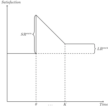
In this set-up, the contemporaneous, or short-run (SR), effect of own income on life satisfaction is given byβ0. In general the long-run (LR) effect is given byP
∞
k=0β0−k, but I assumeβ0−k = 0∀k > K
in the special case of equation (1). Thus in equation (1), theLReffect is given byPK
k=0β0−k. Finally,
P∞
k=1β0−k gives the total effect of adaptation
13
, i.e. the degree to which the effect of income dissipates with time. We may also generally say that adaptation is given by the difference between the long-run and the contemporaneous effect (i.e. ADAP =LR−SR). All of this is illustrated in figure 314
. Of
12In a related vein,Peng(2017) finds that the effects of reference incomes are moderated by individual’s level of income. 13OrPK
k=1β0−kin the case of (1))
14The study ofWolbring et al.(2013), where they also attempt to study adaptation to income in life satisfaction, pursues an altogether different approach. They exclusively use lagged first differences (up to three) and no term for the level of income, i.eLSi,t=γo∆ ln(yt) +γ1∆ ln(yt−1) +γ2∆ ln(yt−2) +φXi,t+µi+ǫi,t. They state that if the effect of the first
Life Satisfaction
Time
=
β
0=
=
P
Kk=1
β
0−k=
P
Kk=0
β
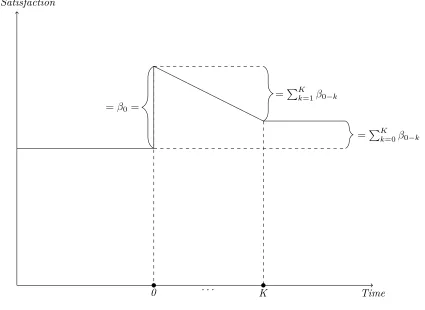
0−k [image:11.612.105.530.86.396.2]0
. . .
K
Figure 3: Illustration of the process modeled in (1) and (2). A positive and persistent income shock in own income is experienced at time zero. I assume partial adaptation.
course, the same reasoning applies to the estimates of theSR, LR,and adaptation effects of reference incomes. When looking for the respective joint effects, I may just take the sums of the effects of own and reference income.
The review in section2has made clear that controlling for (at least some) lagged terms of controls can drastically change results. The reason for this may be as follows: controlling forXitstems from the belief thatXitis correlated withyownit andLSit. If this is so, we must also also believe thatXi,t−kis correlated
withyown
i,t−k. Given the literature on adaptation to various life events (Angeles, 2010;Clark et al.,2008;
Hanglberger and Merz,2011), we may have further reason to believe that at least some variables inXit−k
will also be correlated withLSit
15
. If this is so, my estimates of the long-run, short-run and adaptation effects would have to be biased. In particular, any observed adaptation to income may be driven by unobserved adaptation to changes in any of the covariates in X. Hence I should further extend the model by adding lags of all control variables that are not perfectly collinear with its contemporaneous values16
. This is similar to the approach ofFerrer-i Carbonell and Van Praag(2008) andVendrik(2013). The model thus becomes:
15It may further be that elements in an appropriately constructed vector Xref
it , e.g. levels of unemployment in the
reference group, would behave similarly. I omit this complication from the present investigation.
LSi,t= K X
k=0
β0−kln(yi,t−k) +
K X
k=0
γ0−kln(y
ref i,t−k) +
K X
k=0
φ0−kXi,t−k+µi+τt+ǫi,t (2)
When attempting to compare effects obtained from UKHLS and GSOEP, I restrict the observation window to 1996-2015 for both data-sets to account for the limited coverage of the UKHLS, use the same income concept (at baseline: real net household income)17
, and use comparable controls (seeAppendix table A1). I treat life satisfaction as cardinal rather than ordinal. Ferrer-i Carbonell and Frijters(2004), Van Praag and Ferrer-i Carbonell(2008) orRiedl and Geishecker(2014) showed that treating income as cardinal rather than ordinal makes very little difference to ratios of coefficients and levels of significance.
3.2
Two extensions
Though more robust than the empirical strategy pursued in most other studies (in particular by virtue of the uncommon use of terms for the lags of controls), there are four further objections to this approach that I try to alleviate. First, income is measured with error. Such error may be driven by individuals not being able to accurately report on their income, the need to impute income in some cases, or inaccuracies in the tax-simulation routines used to arrive at net incomes. Such measurement error may lead to attenuation bias towards zero of the estimated own income effects. Second, there may unobserved costs to income generation, such as stress of higher commuting times, which may present a downward bias to the estimated own income effects. Third, there may be effects of covariates lagged further than K years, omission of which will yield biased estimates of all included terms. Fourth, life satisfaction may be an autoregressive process that operates over and above observables. In other words it may be that life satisfaction attis partially caused by life satisfaction at t−1, where the causation is not mediated by any further variables. I now discuss my remedies for these issues.
3.2.1 Instrumenting
To alleviate the first and second concern, I instrument income following the approach first pursued by Luttmer (2005) and later adopted by Luechinger (2009) and Vendrik (2013). This approach goes as follows: For each wave, I predict real individual labor earnings using the respondent’s age, age-squared, gender and a large set of occupation and industry dummies18
. Thus for each wave, I run a regression of the formylabour
i =α+β1M ALE+β2,AGE+β3AGE 2
+δindIN DU ST RYi+φoccOCCU P AT IONi+ǫi., whereδind andφoccare industry- and occupation-specific parameters. In the German case, I use 4-digit ISCO88 codes for occupation, and 2-digit NACE codes for industry. In the UK case, I use 3-digit SOC codes for occupation, and 2-digit SIC codes for industry. In the next step, I sum the predicted earnings of each individual in the household. I then equivalize this measure for household size and use it to instrument for observed equivalized household income.
There are two interrelated threats to the exclusion restriction of this instrument. The first concern is that there may be other time-varying effects on life satisfaction of industry or occupation beyond those
17I choose not to convert Pounds into Euros. Under the assumption that the separate series for inflation used to obtain a household income measure in constant prices in each country are comparable, my use of lns for all income terms in all estimations, as well as my use of year fixed effects, renders such a conversion unnecessary.
of time-varying pecuniary returns. On the one hand, it may be that individuals in the same occupation and industry may form part of the individual’s reference group. Although I control for reference incomes defined over education and age, there may thus nevertheless be an uncontrolled-for negative effect that would downwardly bias the IV estimate. On the other hand, it may be that general work conditions in some industries have gotten better, while pay has increased too. This would lead to an upward bias in the IV estimate.
The second concern is that respondents may choose to select into particular industries or occupations in anticipation of changes in income or other benefits that may impact life satisfaction. Pischke and Schwandt(2012) note that industry choice is indeed correlated with fixed characteristics of individuals. Given my use of the ln of income and my use of individual fixed-effects, selection into industries or occupations that is driven by the overall mean of income (or the mean of other benefits) across the observation window is not a concern. However, when people actively switch industries or occupations in anticipation ofchangesin industry- or occupation-specific pecuniary or non-pecuniary returns, and when the propensity to switch is correlated with unobservables, my estimates may still be biased.
I partially guard against these concerns by later adding contemporaneous and lagged values of all industry and occupation dummies to the model. The inclusion of these dummies then controls for all effects of industry and occupation that do not run via individual labor incomes. In that case, bias may only occur when individuals actively switch industries and occupations in anticipation of hedonic returns (an upward bias), or via negative reference income effects that are captured by my generated income variable (a downward bias).
3.2.2 Addition of lagged life satisfaction
To robustify my main estimates against the third and fourth concern, I, add a term for lagged life satisfaction to the model. This yields an autoregressive distributed lag model of the following form :
LSi,t= K X
k=0
β0−kln(yi,t−k) +
K X
k=0
γ0−kln(y
ref i,t−k) +
K X
k=0
φ0−kXi,t−k+ρLSi,t−1+µi+τt+ǫi,t (3)
Assuming thatρis positive and smaller than 1, this alleviates the same worriesVendrik(2013) seeks to solve with his error-correction model, but is a simpler and more intuitive representation19
. By repeated substitution, equation (3) can be rewritten as follows (for brevity I omit terms for reference income, controls and errors):
LSi,t=β0ln(yi,t) + (β−1+ρβo) ln(yi,t−1) + (β−2+ρβ−1+ρ 2
β0) ln(yi,t−2) +. . . (4)
+ (β−4+ρβ−3+· · ·+ρKβo) ln(yi,t−K) + ∞
X
m=1 ρm(
K X
l=0
ρlβ−K−l) ln(yi,t−K−m) +. . .
Definingβ∗
0−k,γ ∗
0−k, andφ ∗
0−k appropriately this can in turn be rewritten as:
LSi,t=β0ln(yi,t) +
∞
X
k=1 β∗
0−kln(yi,t−k) +γoln(y
ref i,t ) +
∞
X
k=0 γ∗
0−kln(y
ref
i,t−k)+ (5)
φ0−kXi,t+ ∞
X
k=0 φ∗
0−kXi,t−k+µ ∗
i +τ
∗
t +ǫ
∗
i,t
I thus implicitly model the effects of indefinitely long lags of own and reference income, as well as all controls. There are two equivalent sets of assumptions: Life satisfaction, beyond the part that is explicitly modeled, is assumed to be an autoregressive process of order 1, with 0≤ρ <1. Equivalently, beyond those that are explicitly modeled, I assume the effects of income and all controls att−K−mto exponentially decay at rateρmform >0. This homogeneous rate of decay is also assumed for the effects of the unobserved time-varying controls att−K−m for m > 0. The latter is a somewhat stringent assumption.
To obtain theSRk,LR, and adaptation effects, the same formulas as those presented in section3.1 can be applied to equation (5). The sum β0+P
∞
k=1β
∗
0−k, i.e. the long-run effect of own income, can
be expressed as PK
k=0β0−k
1−ρ (the same goes for reference incomes)
20
. Unfortunately, in a fixed effects setting, the OLS estimate ofρ will be downwardly biased for finiteT. I therefore apply the bootstrap bias correction ofDe Vos et al.(2015) to guard against this concern.
Unfortunately,Vendrik(2013) finds a negative small-T bias in the estimate ofρ, which he claims to go beyond the Nickell Bias. This is why he fixatesρ to an estimate he obtains from a balanced panel with T = 21. I face the same problem: When using my full German sample I obtain an estimate of ρ= 0.13. However, when only selecting respondents who are observed in every wave (which thus yields an effectiveT of 29), my estimate ofρincreases to 0.26, which is very close to Vendrik’s estimate of 0.27 (see his discussion on page 146). In turn, when selecting the same subset of respondents, but randomly selecting an observation window of seven periods (which is closest to meanT when using the full set of respondents) for each of these respondents, I get an estimate ofρ= 14. This is thus very close to the estimate obtained from the full set of respondents. I therefore conclude that the smaller estimate of ρ from the full sample indeed arises from a further, unaccounted-for small-T bias21
, and that the larger estimate forρ I obtain whenT = 28 is less biased and not driven by selection effects that could have arisen from either the time periods considered or the set of respondents included. Throughout I therefore fixateρto the estimate which I obtain with largest possibleT.
3.3
Determining the number of lags
A tricky question is what the appropriate number of lags K is. On the one hand, one would wish to include as many lags as possible, in order to make the assumptions made for equations (2) and (3) as plausible as possible. On the other hand, adding more lags is problematic for two reasons: First the addition of each lag causes the loss of a large number of panel observations. Second, levels of income att andt−1 are highly collinear, thus also leading to a loss in efficiency of the estimates. Vendrikdetermines the number of lags by first starting with some very large number of lags. He then conducts F- and t-tests
20To see this, setLSand ln(y) to their unchanging long-run values in equation (3) and rearrange.
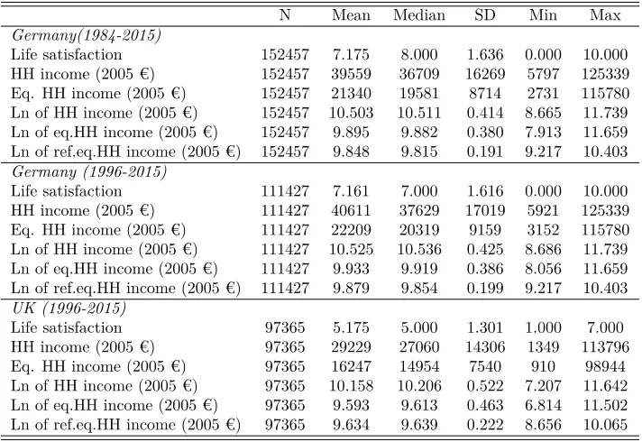
Figure 4: Distribution of life satisfaction in Germany (left) and the UK (right).
of the (joint) significance the highest lag of own and reference income. If all tests fail to reject the null hypothesis of (joint) equality to zero, he removes all highest order lags and repeats the process until he obtains at least one rejection. At baseline, this leads him to use a maximum lag length of 3, while when including lagged life satisfaction and instrumenting for income, he finds an appropriate lag length of 1.
When I apply this approach (using either equation (2) or (3) and instrumenting income) I obtain a lag length of 1 for both the UK and Germany. Given that I have no need to use such a short lag length, I decided to be more conservative and chose a lag-length ofK= 3 for my baseline estimates. This choice is primarily motivated by the observation of this being the maximum lag length at which I continue to obtain a sufficiently large Kleibergen-Paap F-statistic (>10) to get reliable IV estimates for almost all subgroups that I consider. This choice ofK = 3 is much closer to the choice ofDi Tella et al. (2010), Pfaff(2013) andFerrer-i Carbonell and Van Praag (2008) and many others in the literature who use a lag length of four. However, as it turns out, these considerations turn out not to be very important, since my IV results on the full samples are largely robust to lag lengths between 1 and 5 for both the UK and Germany. At higher order lags my instruments become weak in the UK and the reference income effect is estimated rather imprecisely. See tables A4 and A5 in theAppendixfor the relevant regressions.
4
Data
At baseline, I make use of all available GSOEP waves (1-32), spanning the time 1984-2015. For compar-ative purposes, I also use all available waves of the UKHLS, which combines waves 6-1822
of the BHPS
and waves 1-7 of Understanding Society. This translates to the years 1996-2015. Previous work has indicated that incomes at the very top and the very bottom of the income distribution suffer from large measurement error (Berthoud and Bryan, 2011; Figari, 2012). Moreover, self-employed individuals are known to either under- or over-report their incomes (Hurst et al., 2013). For these reasons, I exclude the top and bottom 1% within each wave of household income, as well as all self-employed individuals from the analysis. Since very few individuals younger than 20 years or older than 70 years are observed to have labor earnings (which is needed to instrument household income), I also exclude all individuals that fall outside of this range.
Table 1: Descriptive Statistics
N Mean Median SD Min Max
Germany(1984-2015)
Life satisfaction 152457 7.175 8.000 1.636 0.000 10.000 HH income (2005 €) 152457 39559 36709 16269 5797 125339 Eq. HH income (2005 €) 152457 21340 19581 8714 2731 115780 Ln of HH income (2005 €) 152457 10.503 10.511 0.414 8.665 11.739 Ln of eq.HH income (2005 €) 152457 9.895 9.882 0.380 7.913 11.659 Ln of ref.eq.HH income (2005 €) 152457 9.848 9.815 0.191 9.217 10.403 Germany (1996-2015)
Life satisfaction 111427 7.161 7.000 1.616 0.000 10.000 HH income (2005 €) 111427 40611 37629 17019 5921 125339 Eq. HH income (2005 €) 111427 22209 20319 9159 3152 115780 Ln of HH income (2005 €) 111427 10.525 10.536 0.425 8.686 11.739 Ln of eq.HH income (2005 €) 111427 9.933 9.919 0.386 8.056 11.659 Ln of ref.eq.HH income (2005 €) 111427 9.879 9.854 0.199 9.217 10.403 UK (1996-2015)
Life satisfaction 97365 5.175 5.000 1.301 1.000 7.000 HH income (2005 €) 97365 29229 27060 14306 1349 113796 Eq. HH income (2005 €) 97365 16247 14954 7540 910 98944 Ln of HH income (2005 €) 97365 10.158 10.206 0.522 7.207 11.642 Ln of eq.HH income (2005 €) 97365 9.593 9.613 0.463 6.814 11.502 Ln of ref.eq.HH income (2005 €) 97365 9.634 9.639 0.222 8.656 10.065
household, a weight of 0.5 to every subsequent adult, and a weight of 0.3 for every child in the household. Definitions for all control variables can be found inAppendixtable A1.
Table 1 provides summary statistics for my main variables of interest - household income and life satisfaction. The overall standard deviation of life satisfaction is roughly 1.62 in the German sample, whereas for the British sample it is roughly 1.30. Thus, the ratio of standard deviations (1.62/1.30≈1.25) is reasonably similar to the ratios of the response scales (11/7≈1.57) . This gives further assurance for my comparative purposes23
.
5
Results
5.1
Baseline results for Germany
In this section, I present my results for my baseline estimations of variants of equations (1) and (2) using GSOEP data for the period 1984-2015. In section 5.2, I give results for equations (2) and (3) using instrumented income. Thereafter, in section 5.3, I then estimate similar models for both the UK and Germany on a more restricted time period. In section5.4, I give results for different sub-groups. When I say that an effect or coefficient issignificant, I mean that I obtain a p-value below 0.05. When I say
marginally significant, I mean 0.05≤p <0.1. When I saymarginally insignificant, I mean 0.2> p≥0.1. When I sayinsignificant, I mean p≥0.2.
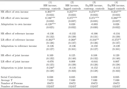
Table 2 gives results for variants of equations (1) and (2). The estimates of column 1 are closest to those ofDi Tella et al.(2010) in that real net household income with contemporaneous controls only are used (i.e. equation (1) is estimated). Like Di Tella et al. (2010), I find significant adaptation to own income that is roughly equal in magnitude to that which they find (-0.120 vs. -0.150; see their table 1 column 2). The contemporaneous effect that I obtain is similar to theirs (0.305 vs. 0.230). However, especially given my much larger samples (I have 15 extra years available), I obtain a significant long-run effect, implying partial rather than full adaptation to own income. Concerning reference incomes, I find an insignificant and negative short-run effect24
. However, the long-run effect is statistically significant, negative and sizable (=-0.262).
In column 2, I again use raw household income to estimate equation (2), which now includes lags of all controls. This extension slightly diminishes the short-run effect of own income. More importantly, however, the long-run effect of own income is now slightly larger than the short-run effect. Thus, all evidence of adaptation observed in column 1 vanishes in column 2. Difference of the same trend were also seen byFerrer-i Carbonell and Van Praag(2008) andVendrik(2013)25
. As explained in section3.1, this suggests that significant adaptation observed in column 1 is the result of omitted variable bias, i.e. adaptation to one of the control variables which are correlated with income. With respect to the effects
23We need not expect these ratios to equal: It may well be that there is less variance in life satisfaction in Germany than in the UK.
24In all regressions I use equivalized reference incomes. When using reference incomes that are not equivalized I find a positive short-run effect and a zero long-run effect. This is in line with the results ofPfaff(2013) in his table B.2, columns 1 and 2. A possible explanation for this is that the effects of household composition of those in the reference group follow a similar dynamic as the effects of the respondent’s own household composition (see main text below): It may be that reference incomes computed on the basis of raw household income pick up (possibly age-specific) variation in the household compositions of the reference group. If so, a positive contemporaneous reference income effect might really just reflect that many in the reference group e.g. marry, which might - if the respondent anticipates to marry soon, too - in turn provide a positive signal to the respondent.
Table 2: Baseline results for equation (2), West Germany (1984-2015)
(1) (2) (3) (4)
HH income, contemp. controls
HH income, lagged controls
Eq.HH income, contemp. controls
Eq.HH income, lagged controls SR effect of own income 0.305*** 0.257*** 0.274*** 0.254***
(0.023) (0.023) (0.023) (0.023)
LR effect of own income 0.186*** 0.277*** 0.271*** 0.280***
(0.032) (0.037) (0.035) (0.037)
Adaptation to own income -0.120*** 0.020 -0.003 0.026
(0.025) (0.032) (0.030) (0.032)
SR effect of reference income -0.136 -0.132 -0.166 -0.134
(0.132) (0.139) (0.131) (0.139)
LR effect of reference income -0.262** -0.268* -0.316** -0.273**
(0.126) (0.137) (0.126) (0.137)
Adaptation to reference income -0.126 -0.136 -0.150 -0.139
(0.127) (0.161) (0.127) (0.161)
SR effect of joint income 0.169 0.125 0.108 0.120
(0.132) (0.140) (0.132) (0.140)
LR effect of joint income -0.076 0.009 -0.044 0.007
(0.125) (0.139) (0.126) (0.138)
Adaptation to joint income -0.246* -0.116 -0.152 -0.113
(0.128) (0.163) (0.128) (0.163)
Serial Correlation 0.038 0.035 0.039 0.035
Average T 7.830 7.830 7.830 7.830
Number of Persons 19472 19472 19472 19472
Number of Observations 152457 152457 152457 152457
of reference incomes, the addition of lagged controls has virtually no effect.
In columns 3 and 4, I perform the same estimations as in column 1 and 2, but use equivalized household income instead. For both columns, my results are very similar to the results of column 2. My estimates of the short-run and long-run effects of own income are roughly equal and hence give no evidence of either adaptation or reinforcement, independent of whether the lags of controls are included or not. My estimates for reference income are again not qualitatively changed in these regressions.
Recall that the joint income effects are simply the sums of the own and reference income effects. These coefficients may be interpreted as the marginal effects of equally sized and permanent income changes of both the respondent and all members of the respondent’s reference group. These estimates therefore give an answer to the question of whether everybody gets happier when everybody gets richer. The answer is no: I generally find positive but insignificant short-run effect, and insignificant (and more negative) long-run effects. All adaptation to joint income is insignificant.
That significant adaptation to own income is observed when using non-equivalized household income and no adaptation is observed when using equivalized household income (and including contemporaneous controls in both cases), is precisely the result that puzzled Pfaff (2013). It may seem odd that the results for non-equivalized household income are very strongly dependent on the inclusion of the lags of controls, while those for equivalized household income are not. However, equivalizing (the lags of) household income implicitly entails controlling for terms for the lags of the variable that determines the equivalization scale, i.e. the numbers of adults and children in the household. This can be seen as follows: Letyeqi,t be equivalized HH income andydef li,t be non-equalized HH income. The equivalization scale is
given byEQi,t≡(1 + (nadultsi,t−1))∗0.5 +nchildreni,t∗0.3. Hence: yi,teq≡ ydef li,t
EQi,t. We can then write the model in, e.g., (2), using equivalized income, as:
LSi,t=
3
X
k=0
β0−k[ln(
ydef li,t−k
EQi,t−k
)] +... (6)
.
We can rewrite this to give:
LSi,t=
3
X
k=0 βinc
0−kln(y
def l i,t−k) +
3
X
k=0
β0comp−k ln(EQi,t−k) +... (7)
with (by assumption) βinc
0−k =−β
comp
0−k . Hence, each income related coefficient in the models using
Given that I use the most comprehensive set of controls in columns (2) and (4), I take these to be my preferred specifications. Notice that the results in these columns are, as one would expect, nearly identical. I therefore conclude that I obtain no valid evidence of adaptation for own income, insignificant reinforcement for reference income, and insignificant adaptation to joint income. The oft-cited evidence of adaptation to own non-equivalized income observed byDi Tella et al.(2010) appears entirely driven by reinforcement of the negative effect of household composition. I further find evidence of significant long-run effects for own (positive) and reference (negative) income, which in conjunction yield an insignificant long-run effect of joint income that is very close to zero. Taken together, these findings support the relative-income explanation for the Easterlin Paradox.
[image:20.612.90.522.282.654.2]5.2
Extended results for Germany
Table 3: Extended results for equation (2) and (3), West Germany (1984-2015)
(1) (2) (3) (4)
Instr.Eq. HH income, lagged controls
Instr.Eq. HH income, lagged controls,
lagged LS
Instr.Eq. HH income, lagged controls, indust. & occup.
Instr.Eq. HH income, lagged controls,
lagged LS, indust. & occup.
Lagged life satisfaction 0.263 0.263
SR effect of own income 0.687*** 0.715*** 0.409** 0.421**
(0.181) (0.188) (0.169) (0.175)
LR effect of own income 0.523*** 0.514*** 0.465*** 0.464***
(0.117) (0.130) (0.118) (0.133)
Adaptation to own income -0.163 -0.201 0.055 0.043
(0.171) (0.180) (0.159) (0.168)
SR effect of reference income -0.203+ -0.267* -0.182+ -0.236*
(0.142) (0.140) (0.142) (0.139)
LR effect of reference income -0.321** -0.352** -0.317** -0.351**
(0.143) (0.152) (0.143) (0.152)
Adaptation to reference income -0.118 -0.085 -0.135 -0.115
(0.166) (0.174) (0.166) (0.174)
SR effect of joint income 0.484** 0.448** 0.227 0.185
(0.207) (0.211) (0.201) (0.204)
LR effect of joint income 0.202+ 0.162 0.148 0.112
(0.156) (0.168) (0.160) (0.173)
Adaptation to joint income -0.282+ -0.286+ -0.080 -0.072
(0.212) (0.221) (0.207) (0.217)
Kleibergen-Paap F statistic 54.945 56.511 67.360 68.450
Serial Correlation 0.029 -0.219 0.028 -0.217
Average T 7.830 7.831 7.830 7.831
Number of Persons 19472 19381 19472 19381
Number of Observations 152457 151765 152457 151765
Estimated with Correia’s ’reghdfe’ command.
Coefficient on lagged life satisfaction obtained with De Vos’ & Ruyssen’s ’xtbcfe’ command. Individual and year fixed-effects & (lagged) controls included.
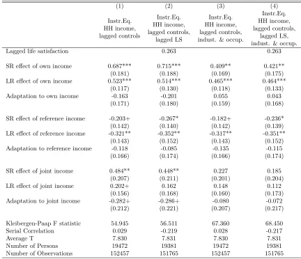
As explained in section 3.2, while more robust and comprehensive than many of the results in the previous literature, the results of section 5.1 may nevertheless suffer from a negative bias in the own income effect via measurement error and unobserved costs to income generation. The results may further suffer from a downward bias in the estimate of adaptation via the omission of higher order lags and biases of unknown direction via the omission of further time varying controls. In table 3, I therefore present estimates in which I try to correct for these potential problems using the approach given in section3.2.
In column 1 of table 3, I take the same specification as that of table 2, column 4, but instrument for all own income terms. This yields long- and short-run effects for own income that are roughly twice the size of the observed own income effects. This difference is roughly in line with the results ofPowdthavee (2010), Luechinger (2009) or Knight and Gunatilaka (2010)26
. Although the long-run effect is now somewhat smaller than the short-run effect, my estimate of adaptation continues to be insignificant (p=0.34). This result contradicts the finding ofVendrik(2013) who finds significant adaptation to own income when instrumenting. In theAppendix(table A2) I investigate the sensitivity of my estimates to the exclusion of each control. That exercise reveals that when I fail to include partner’s employment, I do obtain marginally significant estimates of adaptation. It turns out that there is a large positive contemporaneous effect of partner employment that is subject to full adaptation after three periods. Especially for Women, partner employment is strongly correlated with household income. AsVendrik (2013) does not include partner’s employment status (nor does any other study that I am aware of), it seems that the estimates ofVendrik(2013) also suffer from omitted variable bias27
.
Looking at reference incomes, my effect estimates for both the short-run and the long-run are now slightly larger than in table 2 but qualitatively unaffected. When adding the effects of own income and reference income, I now obtain a large and significant run effect of joint income. This short-run effect of joint income is then subject to (marginally insignificant) adaptation, yielding a marginally insignificant (but positive), long-run effect of joint income.
In column 2, I present my first estimate of equation (3). The inclusion of lagged life satisfaction to the model makes little substantive difference to any of the results28
, albeit yielding a slightly larger estimate for the short-run effect of own income and the effect of reference income (which is now marginally significant). The fact that there is very little change in results when including lagged life satisfaction or not suggests that a lag length ofK = 3 is sufficient if the effects of higher order lags indeed decay exponentially. In table A4 of theAppendixI provide a further test for this. There, I take the specification of table 3, column 1 but let the number of lagsK vary between 1 and 5. This reveals that the effects of own income are indeed robust to changes in the lag length, with my estimate of adaptation always being
26Knight and Gunatilaka(2010) andPowdthavee(2010) use different instruments to the one employed here. Vendrik (2013) andLuechinger(2009) use the same kind of instrument. The fact that different instruments produce similar changes in results when comparing OLS and IV estimates, suggests that it is not a violation of the exclusion restriction that is driving these changes.
27In theAppendix(table A6) I also verify a result from section5.1: When instrumenting forraw, rather thanequivalized household income it is possible to obtain significant evidence of partial adaptation to own income. When, and only when, one fails to include lags for household composition, significant adaptation can be observed there. However, the discussion in section3.1shows that doing so would be mistaken.
28Note, however, how my estimate of first order serial correlation in the residuals turns much more negative with the inclusion of lagged life satisfaction. Under the null of a dynamically complete model in a fixed effects settings, I should expect the serial correlation to equal −1
¯
T−1 (seeWooldridge(2010), p.275). When including lagged life satisfaction in column 2 of table 2 I obtain a deviation from that of 0.07 (= −1
7.83−1−(−)0.22). When failing to include life satisfaction I obtain a
deviation from this expected serial correlation of -0.18 (= −1
7.83−1−0.03). The inclusion of lagged life satisfaction therefore
insignificant. However, it seems as though the long-run reference income effect is not quite as stable, yielding somewhat larger estimates with greater lag lengths. Though this was already suggested by the slightly larger estimated reference income effect found for the dynamic model in column 2 of table 3, these results suggest that the reference income effect may be subject to very slow reinforcement that may take longer than three years. Hence, my estimate of the long-run reference income effect is possibly slightly biased towards zero at baseline for Germany. This also implies that my estimated joint income effect may be somewhat upwardly biased.
Columns 3 and 4 of table 3 address a concern raised in section3.2, namely that the instrument may pick up further non-pecuniary positive effects of industry and occupation choice. I test for this by including contemporaneous and lagged values of all industry and occupation dummies to the regression. In doing, so my instrument can now only pick up the effects of varying pecuniary returns to industry-occupation combinations via their prediction of labor incomes, while all non-pecuniary effects will be captured by the industry and occupation dummies. The inclusion of these dummies depresses the estimates of the short- and long-run effects of own income. Importantly, the estimate of the short-run effect is depressed more than the estimate of the long-run effect, thus now yielding insignificantreinforcement rather than insignificantadaptation. Thus, even the insignificant finding of adaptation in columns 1 and 2 vanishes and reverses sign in these more robust estimations. My results for reference incomes are unaffected by the inclusion of these dummies.
5.3
Main results for comparison of Germany and the UK
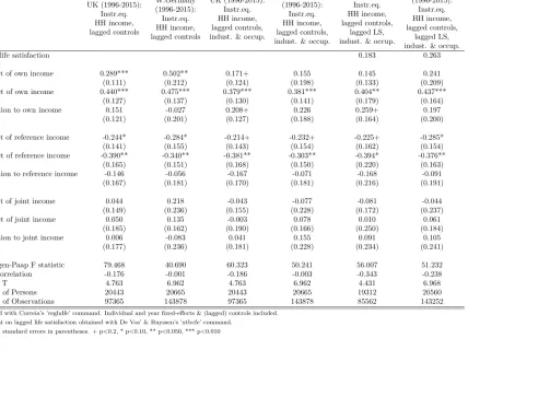
I now turn to comparative results for Germany and the UK. I am not aware of any previous paper in the literature on adaptation in life satisfaction that has been strongly comparative. The working paper by Pfaff(2013) uses the BHPS and GSOEP simultaneously, but is not very comparative. This general lack of cross-country comparison is problematic: Much of the previous happiness literature seems to implicitly view results that are obtained with data from only one country (i.e. Germany with GSOEP) as indicative of facts beyond this particular country (i.e. rich industrialized democracies). Pursuing a comparative approach is an informal test of this presumed external validity. Put differently, in response to a lack of replication and/or replicability in economics and psychology (Earp and Trafimow,2015; Chang and Li, 2018), using UKHLS data alongside GSOEP data can be viewed as a replication of what is thought to be known from GSOEP data. To make results comparable I use the same set of controls for both countries and restrict the estimation period for the German sample to that available for the British sample. Table 4 presents my results.
In columns 1 and 2, I replicate the estimate of table 3 column 1 using UKHLS data and the restricted GSOEP sample. There is no statistically significant evidence of adaptation for either country. Indeed, I observe insignificant reinforcement for the British sample. The coefficient estimate for the UK is somewhat smaller than for Germany. However, given the smaller number of response categories and the smaller standard deviation for life satisfaction in the British data, the substantive long-run effect of own household income appears somewhat larger in the UK than in Germany29
. Turning to reference incomes, I find that the long-run effect of reference income for the restricted German sample is similar to the
29Standardizing effect sizes via the number of response categories yields that the UK effect equals 144% (11/7×0.44 0.48 = 1.46) of the German effect. Standardizing via the respective standard deviations yields that UK’s effect equals 114% of the German effect (1/1.30×0.44
Table 4: Comparative results for variants of equations (2) and (3)
(1) (2) (3) (4) (5) (6)
UK (1996-2015): Instr.eq. HH income, lagged controls
W.Germany (1996-2015): Instr.eq. HH income, lagged controls
UK (1996-2015): Instr.eq. HH income, lagged controls, indust. & occup.
W.Germany (1996-2015): Instr.eq. HH income, lagged controls, indust. & occup.
UK (1996-2015): Instr.eq. HH income, lagged controls,
lagged LS, indust. & occup.
W.Germany (1996-2015): Instr.eq. HH income, lagged controls,
lagged LS, indust. & occup.
Lagged life satisfaction 0.183 0.263
SR effect of own income 0.289*** 0.502** 0.171+ 0.155 0.145 0.241 (0.111) (0.212) (0.124) (0.198) (0.133) (0.209) LR effect of own income 0.440*** 0.475*** 0.379*** 0.381*** 0.404** 0.437***
(0.127) (0.137) (0.130) (0.141) (0.179) (0.164) Adaptation to own income 0.151 -0.027 0.208+ 0.226 0.259+ 0.197
(0.121) (0.201) (0.127) (0.188) (0.164) (0.200)
SR effect of reference income -0.244* -0.284* -0.214+ -0.232+ -0.225+ -0.285* (0.141) (0.155) (0.143) (0.154) (0.162) (0.154) LR effect of reference income -0.390** -0.340** -0.381** -0.303** -0.394* -0.376**
(0.165) (0.151) (0.168) (0.150) (0.220) (0.163) Adaptation to reference income -0.146 -0.056 -0.167 -0.071 -0.168 -0.091
(0.167) (0.181) (0.170) (0.181) (0.216) (0.191)
SR effect of joint income 0.044 0.218 -0.043 -0.077 -0.081 -0.044 (0.149) (0.236) (0.155) (0.228) (0.172) (0.237) LR effect of joint income 0.050 0.135 -0.003 0.078 0.010 0.061
(0.185) (0.162) (0.190) (0.166) (0.250) (0.184) Adaptation to joint income 0.006 -0.083 0.041 0.155 0.091 0.105
(0.177) (0.236) (0.181) (0.228) (0.234) (0.241)
Kleibergen-Paap F statistic 79.468 40.690 60.323 50.241 56.007 51.232 Serial Correlation -0.176 -0.001 -0.186 -0.003 -0.343 -0.238
Average T 4.763 6.962 4.763 6.962 4.431 6.968
Number of Persons 20443 20665 20443 20665 19312 20560
Number of Observations 97365 143878 97365 143878 85562 143252
Estimated with Correia’s ’reghdfe’ command. Individual and year fixed-effects & (lagged) controls included. Coefficient on lagged life satisfaction obtained with De Vos’ & Ruyssen’s ’xtbcfe’ command.
Clustered standard errors in parentheses. + p<0.2, * p<0.10, ** p<0.050, *** p<0.010
the full German sample, yielding a significantly negative effect. Even before standardizing, the long-run reference income effect for the UK is again similar but somewhat larger in absolute size than the German one (-0.39 vs. -0.34). As was the case in table 3, I observe insignificant reinforcement of the reference income effect in both cases.
In columns 3 and 4, I add dummies for each industry and occupation to provide the same check of the instrument as given in the previous section and discussed in section3.2.1. For both countries, this again results in a much diminished short-run effect, but a fairly stable long-run effect for own income. As was the case in the previous section, I now find insignificant reinforcement for Germany rather than insignificant adaptation to own income. My estimates for reference income are again only marginally affected. Finally, columns 5 and 6 give results when further adding lagged life satisfaction, where the coefficient on lagged life satisfaction is fixated in the way described in section 3.2.2. My results are qualitatively robust to this addition.
Throughout all of these analyses, both short- and long-run effects of joint income (i.e. the combined effects of own and reference income) are insignificant in both countries. Thus, it seems that neither in the UK nor in Germany would making everybody richer, make everybody happier. In theAppendixI provide further robustness checks. In table A5, I investigate whether the British estimates are sensitive to lag length. Just as was the case for Germany, my results are largely robust to the choice of the number of lags. In table A7, I reestimated these models with instrumented raw (rather than equivalized) household income. I again find significant adaptation to own income whenever (and only when) I fail to include for household composition. This also agrees with my German results. Finally, table A8 replicates the analysis of table 2 for the UK; thus using observed rather than instrumented own income. This yields very small estimates, which agrees with the results ofPfaff (2013). Given that the BHPS does not directly provide net income data and had to be generated with external information by Levy and Jenkins(2012), it is likely that these estimates using observed income suffer from severe attenuation bias due to measurement error. This indicates that it is paramount to use valid instruments in the case of this British data.
5.4
Results for sub-groups
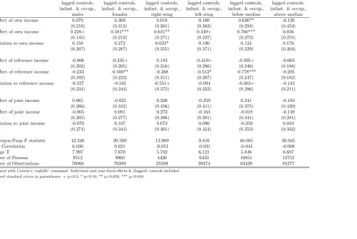
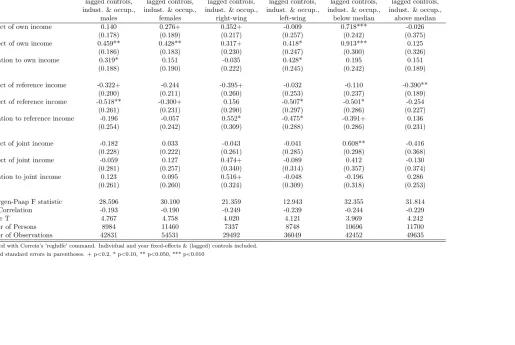
I now turn to investigating whether there are differences across population groups, and whether these differences are homogeneous across the two countries I am investigating. Tables 5 (Germany) and 6 (UK) give results for when I stratify my sample between men and women (columns 1 and 2), those on the political left and right (columns 3 and 4), and those that are either above or below median household income at time of the survey (columns 5 and 6)30
. The first two subgroups were also used in Di Tella et al.(2010), and thus allow for a further attempt at corroboration of these studies’ main findings.
Di Tella et al.(2010) find that only women adapt to own income, and that they fully adapt. As could be expected, I cannot confirm this finding. Instead I find insignificant reinforcement of the own income effect for both men and women, and a much larger positive long-run effect for women than for men31
, the latter of which is even marginally insignificant. Concerning reference income, I also find such stronger
30Apart from restricting the sample, these specifications are the same as those given in table 3 column 4 (Germany), and table 4 column 3 (UK).
Table 5: Results for variants of equation (2) for various subgroups, West Germany (1984-2015)
(1) (2) (3) (4) (5) (6)
Instr.Eq. HH income, lagged controls, indust. & occup.,
males
Instr.Eq. HH income, lagged controls, indust. & occup.,
females
Instr.Eq. HH income, lagged controls, indust. & occup.,
right-wing
Instr.Eq. HH income, lagged controls, indust. & occup.,
left-wing
Instr.Eq. HH income, lagged controls, indust. & occup.,
below median
Instr.Eq. HH income, lagged controls, indust. & occup.,
above median SR effect of own income 0.070 0.309 0.018 0.160 0.636** -0.120
(0.216) (0.313) (0.361) (0.383) (0.293) (0.453) LR effect of own income 0.228+ 0.581*** 0.641** 0.349+ 0.760*** 0.056
(0.145) (0.213) (0.271) (0.237) (0.273) (0.255) Adaptation to own income 0.158 0.272 0.623* 0.190 0.124 0.176
(0.207) (0.287) (0.355) (0.371) (0.229) (0.304)
SR effect of reference income -0.006 -0.335+ 0.183 -0.419+ -0.395+ -0.063 (0.202) (0.205) (0.316) (0.286) (0.246) (0.188) LR effect of reference income -0.233 -0.500** -0.368 -0.513* -0.778*** -0.205
(0.192) (0.223) (0.311) (0.267) (0.247) (0.182) Adaptation to reference income -0.227 -0.165 -0.551+ -0.094 -0.383+ -0.142
(0.234) (0.244) (0.372) (0.333) (0.296) (0.211)
SR effect of joint income 0.065 -0.025 0.200 -0.259 0.241 -0.183 (0.266) (0.342) (0.456) (0.411) (0.375) (0.439) LR effect of joint income -0.005 0.081 0.273 -0.163 -0.018 -0.149
(0.205) (0.277) (0.386) (0.301) (0.341) (0.281) Adaptation to joint income -0.070 0.107 0.073 0.096 -0.259 0.034
(0.274) (0.344) (0.461) (0.424) (0.353) (0.332)
Kleibergen-Paap F statistic 42.346 20.599 12.989 9.816 40.085 30.045 Serial Correlation 0.030 0.021 -0.052 -0.031 -0.044 -0.008
Average T 7.997 7.670 5.782 6.121 5.846 6.687
Number of Persons 9512 9960 4426 6433 10851 12752
Number of Observations 76068 76389 25589 39374 63439 85277
Estimated with Correia’s ’reghdfe’ command. Individual and year fixed-effects & (lagged) controls included. Clustered standard errors in parentheses. + p<0.2, * p<0.10, ** p<0.050, *** p<0.010
Table 6: Results for variants of equation (2) for various subgroups, UK (1996-2015)
(1) (2) (3) (4) (5) (6)
Instr.Eq. HH income, lagged controls, indust. & occup.,
males
Instr.Eq. HH income, lagged controls, indust. & occup.,
females
Instr.Eq. HH income, lagged controls, indust. & occup.,
right-wing
Instr.Eq. HH income, lagged controls, indust. & occup.,
left-wing
Instr.Eq. HH income, lagged controls, indust. & occup.,
below median
Instr.Eq. HH income, lagged controls, indust. & occup.,
above median SR effect of own income 0.140 0.276+ 0.352+ -0.009 0.718*** -0.026
(0.178) (0.189) (0.217) (0.257) (0.242) (0.375) LR effect of own income 0.459** 0.428** 0.317+ 0.418* 0.913*** 0.125
(0.186) (0.183) (0.230) (0.247) (0.300) (0.326) Adaptation to own income 0.319* 0.151 -0.035 0.428* 0.195 0.151
(0.188) (0.190) (0.222) (0.245) (0.242) (0.189)
SR effect of reference income -0.322+ -0.244 -0.395+ -0.032 -0.110 -0.390** (0.200) (0.211) (0.260) (0.253) (0.237) (