Hubless Nearest Neighbor Search for Bilingual Lexicon Induction

Proceedings of the 57th Annual Meeting of the Association for Computational Linguistics, pages 4072–4080 4072

Hubless Nearest Neighbor Search for Bilingual Lexicon Induction

Jiaji Huang∗ Qiang Qiu† Kenneth Church∗ ∗

Baidu Research, Sunnyvale, CA, 94089

†_{Department of Electrical Engineering, Duke University, Durham, NC, 27707}

∗_{

huangjiaji, kennethchurch}@baidu.com †[email protected]

Abstract

Bilingual Lexicon Induction (BLI) is the task of translating words from corpora in two lan-guages. Recent advances in BLI work by aligning the two word embedding spaces. Fol-lowing that, a key step is to retrieve the near-est neighbor (NN) in the target space given the source word. However, a phenomenon called hubness often degrades the accuracy of NN. Hubness appears as some data points, called hubs, being extra-ordinarily close to many of the other data points. Reducing hubness is necessary for retrieval tasks. One successful example is Inverted SoFtmax (ISF), recently proposed to improve NN. This work pro-poses a new method, Hubless Nearest Neigh-bor (HNN), to mitigate hubness. HNN dif-fers from NN by imposing an additionalequal preference assumption. Moreover, the HNN formulation explains why ISF works as well as it does. Empirical results demonstrate that HNN outperforms NN, ISF and other state-of-the-art. For reproducibility and follow-ups, we have published all code1_.

1 Introduction

This paper presents a new method for Bilingual Lexicon Induction (BLI), which we call Hub-less Nearest Neighbor (HNN). BLI is the task of creating a lexicon of translation equivalents such as,bank:bancorbank:banqueautomatically from non-parallel corpora. The proposed method not only improves upon but also unifies several recent works that retrieve translations by Near-est Neighbor (NN) (Mikolov et al., 2013) and more advanced techniques likeInverted SoFtmax (ISF) (Smith et al.,2017).

There is a long history of BLI using non-parallel corpora. Methods often rely on some designed features, which reveal some shared

1_{https://github.com/baidu-research/HNN}

structures across languages. For example, co-occurrence matrices (Rapp, 1995), tf-idf of con-text words (Fung, 1998), and lexical similari-ties (Klementiev et al., 2012). A comprehensive study can be found in (Irvine and Callison-Burch,

2017).

Recently,Mikolov et al.(2013) observe that iso-morphism exists across word embeddings of dif-ferent languages. This motivates them to learn a linear mapping to align the spaces, using a seed-ing dictionary of 5K pairs of translations. Af-ter that, more translations can be induced by NN search. Following the seminal work, significant advances have been made. For example, Faruqui and Dyer(2014) use Canonical Component Anal-ysis to align the two embedding spaces. Xing et al.(2015) show a substantial gain by normaliz-ing the embeddnormaliz-ings and constrainnormaliz-ing the mappnormaliz-ing to be orthogonal. A series of works by Artetxe et al. (2017, 2018a,b) show that decent accura-cies can be achieved even with a tiny or no seed-ing dictionary. The authors name their method as “self-learning”, which alternates between learning the mapping and inducing more translation pairs. The similar methodology is also seen in (Zhang et al.,2017b), where the induction step reduces a cost called earth mover distance. Conneau et al.

(2018) propose to use Generative Adversarial Net-work (Goodfellow et al.,2014) to learn the map-ping when no seeding dictionary is available.

2011; Suzuki et al., 2013; Zhang et al., 2017a), including BLI (Dinu et al., 2014). Recently, re-markable improvements have been made in BLI by mitigating hubness. For example,Smith et al.

(2017) propose Inverted SoFtmax (ISF) that scales the similarities by a (global) measure of hubness.

Conneau et al. (2018) develop a method called Cross domain Similarity Local Scaling (CSLS) that relies on a local measure of hubness instead.

This work studies how to overcome hubness in BLI. The new method, HNN, is proposed by in-troducing anequal preference assumption. As we shall see, the assumption leads to an optimization problem that manifests the connection between HNN, NN and ISF. Empirical results demonstrate that HNN is very competitive and able to outper-form NN, ISF and other state-of-the-art like CSLS. In summary, the paper makes the following contri-butions:

1. We propose an optimization based frame-work that connects NN, ISF and the proposed HNN.

2. We derive an efficient solver for HNN, which outperforms NN, ISF and other state-of-the-art.

3. We show that ISF is a part of HNN’s solver, which explains why ISF works.

2 Bilingual Lexicon Induction with a Seeding Dictionary

Since hubness is the major concern of this work, we focus on the case with a seeding dictionary for simplicity. Representative methods (Mikolov et al., 2013; Xing et al., 2015; Artetxe et al.,

2018a) often consist of two steps: 1) learning a mapping that aligns the source and target embed-ding spaces; 2) given a source word, retrieve ac-cording to some distance metric, in the target em-bedding space. We briefly review the two steps in this section.

Let the source word embeddings space beX ⊂

Rd, and the target space be Y ⊂ Rd. A

typi-cal value of the dimensiondis 300. Suppose the vocabulary sizes of source/target languages arem andnrespectively. ThenX is a set ofm embed-ding vectors, denoted as

X ={x1, . . . ,xm}, andYis a set ofnembeddings,

Y ={y1, . . . ,yn}.

2.1 Learning Linear Transformation

Suppose we can access a seeding dictionary, which reveals some correspondences from a sub-set of X to a subset of Y. The correspondence can be one-to-one, many-to-one, or one-to-many. In matrix form, let the columns of matrixX (Y) be the embeddings of source (target) words in the dictionary, where thej-th columns ofXandYare the embeddings of a pair of translations.

Using X and Y, a linear mapping T can be learned, which “aligns” the X and Y space. In particular,

T= arg min

T∈Ω

kTX−Yk2_F.

Here Ω is a constraint set on T. For exam-ple, Mikolov et al.(2013) simply let Ωbe Rd×d,

whereasXing et al.(2015) show substantial gain by settingΩas the set of orthogonal matrices.

2.2 Retrieval by Nearest Neighbor (NN)

Once theTis obtained, translation can be cast as a retrieval problem. We define a distance matrix

D, between the mapped source embeddings and target embeddings,

Di,j ,dist(Txi,yj),

where “dist” is some distance metric. For the i-th source word, Nearest Neighbor (NN) criterion determines (the index of) its translation in the Y

set, by

arg min

j

Di,j (NN)

However, several works (Radovanovic et al.,

2010;Dinu et al.,2014) have observed that the ac-curacy of NN is often significantly degraded by a phenomenon called hubness. Mitigating hubness has thus become necessary, which we will review next.

2.3 Inverted Softmax: Improve NN by

Mitigating Hubness

Hubness occurs in high dimensional feature space (Radovanovic et al., 2010). It appears as some data points, called hubs, being close to too many of the others. We look into Inverted SoFt-max (ISF) (Smith et al., 2017), a recent retrieval methods that tackle hubness.

j-th target. A “temperature” parameteris intro-duced to construct a kernel, exp(−Di,j/). The ISF matrix is obtained by normalizing the ker-nel’s columns first, and then the rows.

ISF(D)i,j =

exp (−Di,j/) ZiPmi=1exp (−Di,j/)

,

where Zi is a row normalizer such that

P

jISFi,j = 1for any i. The (index of) trans-lation for thei-th source word is then determined by

arg max

j

ISF(D)i,j. (ISF)

Smith et al. (2017) show that ISF significantly outperforms NN in BLI tasks. However, it is still not clear why ISF works so well. One contribution of our work is to shed light on the mechanism be-hind ISF, which will be manifested after we study the proposed Hubless Nearest Neighbor.

3 Hubless Nearest Neighbor (HNN)

This section formalizes the proposed HNN. As will be clear from this section and the next, there is a unified view over NN, ISF and HNN. We now start by rephrasing the retrieval task into the fol-lowing general problem. Given the distance ma-trixD defined in section2.2, we seek an assign-ment matrix P where Pi,j is the probability of the j-th target word being the translation of the i-th source word. Assume the target vocabulary is large enough so that one or more translations can always be found for any source word. Therefore

X

j

Pi,j = 1.

The (index of) translation is inferred by

arg max

j

Pi,j.

The art is to determinePfromDand various other information/priors. The above framework is gen-eral in the sense that various designs exist in seek-ing theP.

3.1 NN as a Warm-up

As a warm-up, we show that NN is a special case of the above framework. In specific, let h·,·i be matrix inner product, thenhD,Piis a measure of cost to translate from source to target, which we may want to minimize. In addition, if we mini-mize it along with a negative entropy regularizer (on P), we can reduce the gap between NN and (ISF). As stated by the following proposition,

Proposition 1. The(NN) criterion is equivalent

to arg max_jPi,j, where P is the solution of the following optimization problem,

min

P hD,Pi+

X

i,j

Pi,jlogPi,j

s.t.Pi,j ≥0, X

j

Pi,j = 1

. (P₀)

Proof. The solution to (P₀) is simply

Pi,j =

exp(−Di,j/) Pn

j=1exp(−Di,j/)

. (1)

Substituting Eq. (1) toarg max_jPi,j, we arrive at

arg minDi,j,

which is exactly the NN criterion.

The objective of (P₀) is regularized by P

i,jPi,jlog(Pi,j), which is the negative entropy ofP. It smooths the linear objective, and leads to a solution, Eq. (1), as anther view of NN that is closer to (ISF).

3.2 Equal Preference Assumption

Starting from (P0), we now try to reduce the hubs.

Since hubness results in someyj’s being retrieved more frequently than others, a natural idea is to force all yj’s being equally preferred to be re-trieved. The preference ofyj can be measured by

pfj(P), 1

m X

i Pi,j.

In other words, on average, how the j-th target word is likely to be picked as the translation of a source word. We therefore force _m1 P

iPi,j to be uniform over all j’s. In addition, with the constraint that P

jPi,j = 1 for any i, we have 1

m P

iPi,j = _n1 for anyj. We term the constraint as equal preference assumption. Formally,

Definition 1. Equal Preference Assumption:

pfj =

1

n,

for allj’s.

P∗using an English-French dictionary2. The dic-tionary includes 113K items, with plenty of poly-semies. The vocabularies are built from monolin-gual word embedding files3. Vocabulary sizes are set asm=n= 500,000. TheP∗is computed as

P_i,j∗ , 1

Zi

·

 



1 i-th source word can be translated to thej-th target

0 otherwise

,

(2) whereZiis a normalizer that ensuresPjPi,j∗ = 1. We compute the pfj values using the P∗. To measure how much the values deviate from the equal preference assumption, we compute their variance,

varj[pfj]. (3)

If the equal preference assumption exactly holds, varj[pfj] = 0. Otherwise, the larger the variance, the less true the assumption is. It turns out that varj[pfj]≈1.9×10−11, which is tiny and support the assumption.

3.3 HNN

We add the equal preference assumption as a con-straint to problem (P0), and now solve the

follow-ing new problem instead,

min

P hD,Pi+

X

i,j

Pi,jlogPi,j

s.t.Pi,j ≥0, X

j

Pi,j = 1,

1

m X

i

Pi,j =

1

n .

(P₁) In analogous to (NN) and Proposition1, we intro-duce the following definition of Hubless Nearest Neighbor (HNN).

Definition 2. HNN is the criterion that retrieves

index

arg max

j

Pi,j

wherePis the solution of problem(P₁).

The remaining question is how to solve (P₁), which we will discuss in the next section.

4 Solvers for HNN

We first present a straightforward but less efficient solver, then we derive an efficient alternative. Both solvers, as will be seen, have strong connections with ISF.

2

https://dl.fbaipublicfiles.com/arrival/ dictionaries/en-fr.txt

3

https://dl.fbaipublicfiles.com/fasttext/ vectors-wiki/wiki.en.vecand

https://dl.fbaipublicfiles.com/fasttext/ vectors-wiki/wiki.fr.vec

4.1 A Less Efficient Solver

(P1) can be solved by Sinkhorn iteration (Cuturi, 2013), which iteratively normalizes the columns and rows of a kernel matrix. The steps are sum-marized in algorithm1.

Algorithm 1Sinkhorn Solver for Problem (P₁)

Input: D

Output: P

1: P←exp(−D/)whereexpis on elements.

2: whilestopping criteria not metdo

3: // normalize columns 4: P←Pdiag_m

n./(P

>₁₎ 5: // normalize rows

6: P←diag{1./(P1)}P

7: end while

Here ./ denotes elementwise division, 1 is an all-one vector of suitable length, and diag{·} con-structs a diagonal matrix from a vector.

Remark 1. The Sinkhorn Solver reveals some

connection between ISF and HNN. Indeed, ISF is equivalent to running a single iteration of algo-rithm 1. A deeper connection will be revealed in the next subsection, where we provide a comple-mentary view of problem(P1).

4.2 Dual Problem and an Efficient Solver

One drawback of algorithm 1 is its prohibitive memory cost. Indeed, the Pmatrix has to be in memory for frequent update, which is costly when the vocabulary sizes m and n are big. In this section, we study a dual form of problem (P1),

given in Proposition 2, which hints a more effi-cient method to solve forP.

Proposition 2. The solution of problem(P1) can

be expressed as

Pi,j =

expβj−Di,j

P jexp

_β

j−Di,j

, (4)

whereβjis the solution of

min

β

1

m X

i 

log X

j

exp

βj−Di,j

−1

n X

j βj



Proof. The proof is by method of Lagrangian mul-tipliers. Details are in supplementary.

The dual form (D) is a special case of the dual forms in general contexts (Genevay et al.,2016). (D) is useful because it allows us to learn a much smaller vectorβ(of sizen), instead of keeping up-dating the huge matrixP(mbyn). Moreover, its loss function is a summation over thei’s, which can be minimized by parallelizable gradient de-scent. Finally, (D) is convex, which guarantees the convergence of gradient descent.

It is now a natural idea to derive the gradient of (D) and give a gradient descent solver. Let us define the objective in (D) as`i,

`i,log X

j

exp

βj−Di,j

− 1

n X

j βj.

Then,

∂`i ∂βj

=

expβj−Di,j

P jexp

_β

j−Di,j

−

1

n. (5)

Algorithm 2 summarizes the gradient descent solver. The equivalence between algorithm1and

2 will be empirically validated in section5.1. In large-scale experiments, we apply algorithm2 (in-stead of algorithm1) for its lower memory cost.

Algorithm 2Dual Solver for Problem (P₁)

Input: D, learning rateη.

Output: P

1: β←0

2: whilestopping criteria not metdo

3: fori= 1, . . . , mdo

4: // parallelizable

5: Compute gradient∇`iusing E.q. (5).

6: end for

7: β←β−η· 1 m

P i∇`i

8: end while

9: ComputePby E.q. (4) and return.

Remark 2(Unifying NN, ISF and HNN).

Com-paring thePmatrix under NN (Eq.(1)) and HNN criterion (Eq. (4)), we observe that HNN intro-duces an additional set of values,βj’s. The quan-tity, exp(−βj/), normalizes the j-th column of the kernel matrixexp(−Di,j/). In contrast,(ISF) simply sets the column normalizer as the column

sum, P

iexp(−Di,j/). Obviously, HNN works

harder in figuring out the normalizers, which re-sults in a higher accuracy, as we shall see in the experiment section.

5 Experiments

In this section, we first experiment with synthetic data to illustrate the connection between NN, ISF and the proposed HNN. Then, we report extensive results on BLI task to show the advantage of HNN over NN, ISF and CSLS, another state-of-the-art.

We will also demonstrate that hubness is in-deed reduced by HNN. To measure hubness, we adopt the k-occurrence metric proposed in (Radovanovic et al., 2010), but with a small adaption. In its original definition,k-occurrence, Nk, is the number of times a data point appears among theknearest neighbors of all the others. In our case, we measure for every target example, the number of times it is retrieved against the source set. If a target example is retrieved too many times, it is likely to be a “hub”. For both the original def-inition and our adapted one, hubness can be indi-cated by a long tail of the distribution ofNk.

5.1 Connection between NN, ISF and HNN

We simulate a retrieval task, where source and tar-get spaces are already aligned. In specific, data is generated from a Gaussian mixture model,

10,000

X

c=1

1

10,000· N(µc, 0.01×Id),

where the dimensiond= 300. The class meanµ_c

is generated by normalizing aR300 vector where

each dimension is drawn from uniform(−1,1). We generate two samples per class, one in the source set, the other as the target to be retrieved. We use NN, ISF and HNN with algorithm1 and

2to retrieve for the10K source samples. is set to0.1, which gives the best accuracy of ISF. The sameis also used in HNN.

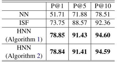
Table1reports top-1, top-5, top-10 accuracies. The two algorithms for HNN achieve the best re-sults and their accuracies are basically the same, validating their equivalence. To understand the improvement over NN, we measure the hubness in different methods. Figure1plots the distribution ofN1, the 1-occurrences. HNN has the shortest tail, in stark contrast to the long tail of NN, imply-ing significantly reduced number of hubs.

5 10 N1 0.0

0.2 0.4

p(

N1

)

NN ISF HNN

Figure 1: Distribution of N1 (1-occurrences): the number of times a target example is retrieved. Longer tail indicates more hubs.

0 10 20 30 iteration

74 76 78

P@1

ISF HNN

Figure 2: P@1 over the iterations in algorithm1. ISF’s P@1 overlaps with that of HNN at the 1st itera-tion.

0 5000_j 10000 −10

0 10

no

rm

ali

ze

r ISFHNN

Figure 3: Hubness normalizers in log domain:logP

iexp(−Di,j/)

for ISF, and −βj/ for HNN,

which is smoother.

Table 1: Compare NN, ISF and HNN on the simulated retrieval task

P@1 P@5 P@10

NN 51.71 71.88 78.51

ISF 73.75 88.57 92.36

HNN

78.85 91.43 94.60

(Algorithm1) HNN

78.84 91.41 94.59

(Algorithm2)

over the iterations in algorithm 1. The accuracy at the first iteration matches that of ISF, validat-ing the comments in remark 1. Next, recall the observation we made in remark 2: Algorithm 2

and ISF both seek normalizers over the target ex-amples to penalize hubness. It is therefore inter-esting to compare the two normalizers, shown in figure3. We observe that the normalizer by HNN is smoother than that of ISF.

5.2 BLI Data and Setups

We now compare the different methods on real BLI tasks. We follow the setup in (Conneau et al.,

2018). The word embeddings and groundtruth dictionaries (for both training and testing) can be downloaded from the MUSE4 repository. The dataset includes word embeddings for 45 lan-guages. We focus on six languages in our experi-ments, since dictionaries are available for any two out of the six. These six languages are English (en), Spanish (es), French (fr), Italian (it), Por-tuguese (pt) and German (de).

Dictionaries for a pair of languages have the fol-lowing three parts:

4

https://github.com/facebookresearch/MUSE

1. src-tgt.0-5000.txt is aseeding dictionaryfor learning the mapping, which has 5K unique source words.

2. src-tgt.5000-6500.txt is a small test dictio-narythat includes 1.5K unique source words. In (Conneau et al.,2018), P@1 values are re-ported on this set.

3. src-tgt.txt is a full dictionary that includes the above two dictionaries and much more src-to-tgt translations. In later experiments, we will use it as alarge test dictionaryby excluding from it the items in src-tgt.0-5000.txt.

Following (Conneau et al.,2018), an orthonor-mal mappingTis learned using the seeding dictio-nary first. The retrieval step uses cosine distance, i.e.,

Di,j = 1 2 1−

y>_j Txi

kxikkyjk !

. (6)

The hyper-parameters (for ISF and HNN,kfor CSLS) should be set as the ones that achieve the best accuracy on the seeding dictionary. We choose to trust the default values ( = 1/30 and k = 10) used in the MUSE repository, since us-ing them, we can reproduce the results reported in (Conneau et al., 2018). For HNN, is set to the same value as in ISF, and we use the gradient solver (Algorithm2) throughout.

en es frtargetit pt de en

es fr it pt de

so

ur

ce

0.0 0.4 0.8 1.2 1.6 2.0 2.4 2.8 3.2 1e−11

(a) varj(pfj)

100 ₁₀1 ₁₀2 ₁₀3 N5

10−6 10−4 10−2

p(

N5

)

NN ISF CSLS HNN

(b) es-en

100 ₁₀1 ₁₀2 ₁₀3 N5

10−6 10−4 10−2

p(

N5

)

NN ISF CSLS HNN

(c) fr-en

100 ₁₀1 ₁₀2 ₁₀3 N5

10−6 10−4 10−2

p(

N5

)

NN ISF CSLS HNN

(d) it-en

100 ₁₀1 ₁₀2 ₁₀3 N5

10−6 10−4 10−2

p(

N5

)

NN ISF CSLS HNN

(e) pt-en

100 ₁₀1 ₁₀2 ₁₀3 N5

10−6 10−4 10−2

p(

N5

)

NN ISF CSLS HNN

(f) de-en

Figure 4: Diagnostics to understand the results in Table3: (a) Visualizing varj[pfj], for every pair of source and

target languages, the corresponding block color-codes the variance of the preferences over the target words. The variances are significantly bigger for pairs that involve German; (b)-(f): Distribution ofN5, the5-occurrences for different methods in foreign-English BLI tasks.5-occurrence is the number of times a target word appears in the top-5 retrievals. Long tail of the distribution indicates hubness.

Table 2: Compare HNN with some reproduced results in Tab.1 of (Conneau et al.,2018), using 200K vocabu-lary. P@1 is reported on the small 1.5K test dictionary. HNN is comparable with ISF and CSLS. Note that the P@1’s are reported on the small test dictionary, which is less convincing. For more convincing comparisons, refer to table3and table 1 in supplementary.

en-es es-en en-fr fr-en

NN 77.40 77.27 74.93 76.07

ISF 81.06 82.60 81.07 81.33

CSLS 81.40 82.87 81.07 82.40

HNN 81.27 82.53 81.33 82.00

5.3 BLI Results on the Large Test Dictionary

Reporting P@1 on the 1.5K small test dictionary may not be sufficient to make a convincing com-parison. We therefore repeat the same experiments but report P@1 on the large test dictionary.

We first keep the vocabulary size of 200K, then try a more challenging 500K. P@1 values are re-ported on the large test dictionary. In fact, results have the same trend for these different vocabulary sizes. Therefore, considering space limit, we put

the results for the 200K case in supplementary. Results of the 500K case are in Tab.3.

HNN outperforms all the other methods in all cases except pairs that involve German. Note that French, Italian, and Portuguese are all Romance languages. German is a Germanic language. En-glish originates from both. The results seem to suggest that the equal preference assumption is not true between Romance and Germanic languages.

To better understand this, we estimate the “groundtruth” preference of target words, and the variance of the preferences, following the process in section3.2(Eq. (2) and (3)). The larger the vari-ance, the less likely the equal preference assump-tion holds. We visualize the variance between any pair of languages in figure4a, where a hot block indicates large variance. We observe a large vari-ance when either the source or target language is German. In other words, the equal preference as-sumption is more violated when translating from or to German.

5.4 Analysis of Hubs in BLI

Table 3: P@1 values on the large test dictionary. Source and target vocabularies are both 500K. HNN is the best except pairs that involve German.

source

target

en es fr it pt de

en

NN 54.98 55.66 46.30 37.02 53.03

ISF 70.35 72.31 63.75 53.02 65.75

CSLS 71.21 72.62 64.11 53.54 66.50

HNN 71.34 73.65 64.91 54.03 64.61

es

NN 59.87 60.76 61.95 66.94 48.73

ISF 73.11 76.82 76.33 78.67 61.70

CSLS 73.02 76.44 76.44 80.29 62.29

HNN 74.38 78.24 77.86 81.09 60.78

fr

NN 61.60 61.73 59.43 46.31 57.10

ISF 74.46 75.72 73.78 60.89 69.07

CSLS 74.88 76.68 74.34 62.06 70.34

HNN 75.97 77.23 75.12 63.10 67.94

it

NN 51.38 64.63 61.45 51.91 50.68

ISF 65.57 77.76 76.64 67.32 63.58

CSLS 65.32 78.45 76.74 68.85 64.57

HNN 67.57 79.75 78.56 70.33 62.96

pt

NN 42.21 68.93 47.48 50.98 37.95

ISF 55.76 81.67 64.37 68.37 51.07

CSLS 54.75 81.98 63.68 67.92 51.78

HNN 57.43 83.97 66.19 70.44 49.93

de

NN 56.06 44.33 52.78 45.44 33.20

ISF 69.74 60.77 71.59 65.99 52.74

CSLS 68.65 59.21 69.88 63.69 50.72

HNN 69.20 60.22 70.71 65.09 52.08

the distribution of theN5values for all methods on foreign-to-English BLI tasks. HNN has the short-est tail in all cases, indicating the fewshort-est hubs.

Table 4: Some representative hubs when applying NN for the pt-en BLI task. Note that the N5 values are significantly reduced after applying HNN.

word N5 N5 frequency

by NN by HNN rank

conspersus 1,776 0 484,387

oryzopsis 1,235 5 472,161

these 1,042 25 122

s+bd 912 16 440,835

were 798 24 40

you 474 20 50

would 467 40 73

It is interesting to see what types of words are likely to be hubs. Table 4lists some representa-tive ones in the pt-en experiment, picked from the top 100 hubs with the biggest N5 values. Some

of them are extremely low-frequency words, e.g., “s+bd”. This is consistent with the finding in (Dinu et al., 2014). However, it is also interest-ing to see that highly frequent words like “were” and “you” also appear to be hubs. Finally, all the N5values are reduced after applying HNN.

6 Conclusion

References

Mikel Artetxe, Gorka Labaka, and Eneko Agirre. 2017. Learning bilingual word embeddings with (almost) no bilingual data. Inthe 55th Annual Meeting of the Association for Computational Linguistics.

Mikel Artetxe, Gorka Labaka, and Eneko Agirre. 2018a. Generalizing and improving bilingual word embedding mappings with a multi-step framework of linear transformations. In32nd AAAI Conference on Artificial Intelligence.

Mikel Artetxe, Gorka Labaka, and Eneko Agirre. 2018b. A robust self-learning method for fully un-supervised cross-lingual mappings of word embed-dings. Inthe 56th Annual Meeting of the Association for Computational Linguistics.

Jean-Julien Aucouturier and Francois Pachet. 2008. A scale-free distribution of false positives for a large class of audio similarity measures. Pattern recogni-tion, 41(1):272–284.

Alexis Conneau, Guillaume Lample, Marc’Aurelio Ranzato, Ludovic Denoyer, and Herv´e J´egou. 2018. Word translation without parallel data. In Interna-tional Conference on Learning Representations.

M. Cuturi. 2013. Sinkhorn distances: Lightspeed com-putation of optimal transport. InAdvances in neural information processing systems.

Georgiana Dinu, Angeliki Lazaridou, and Marco Ba-roni. 2014. Improving zero-shot learning by miti-gating the hubness problem. arXiv:1412.6568.

Manaal Faruqui and Chris Dyer. 2014. Improving vec-tor space word representations using multilingual correlation. Inthe 14th Conference of the European Chapter of the Association for Computational Lin-guistics.

Pascale Fung. 1998. A statistical view on bilingual lexicon extraction: from parallel corpora to non-parallel corpora. InAssociation for Machine Trans-lation in the Americas.

Aude Genevay, Marco Cuturi, Gabriel Peyr´e, and Fran-cis Bach. 2016. Stochastic optimization for large-scale optimal transport. InAdvances in neural in-formation processing systems.

Ian Goodfellow, Jean Pouget-Abadie, Mehdi Mirza, Bing Xu, David Warde-Farley, Sherjil Ozair, Aaron Courville, and Yoshua Bengio. 2014. Generative ad-versarial nets. In Advances in neural information processing systems.

Ann Irvine and Chris Callison-Burch. 2017. A com-prehensive analysis of bilingual lexicon induction.

Computational Linguistics, 43(2):273–310.

Alexandre Klementiev, Ann Irvine, Chris Callison-Burch, and David Yarowsky. 2012. Toward statisti-cal machine translation without parallel corpora. In

the 13th Conference of the European Chapter of the Association for Computational Linguistics.

Tomas Mikolov, Quoc V. Le, and Ilya Sutskever. 2013. Exploiting similarities among languages for ma-chine translation. arXiv preprint arXiv:1309.4168.

Kohei Ozaki, Masashi Shimbo, Mamoru Komachi, and Yuji Matsumoto. 2011. Using the mutual k-nearest neighbor graphs for semi-supervised classification of natural language data. Inthe 15th conference on computational natural language learning. Associa-tion for ComputaAssocia-tional Linguistics, pages 154–162.

Milos Radovanovic, Alexandros Nanopoulos, and Mir-jana Ivanovic. 2010. Hubs in space: Popular nearest neighbors in high-dimensional data. Journal of Ma-chine Learning Research.

Reinhard Rapp. 1995. Identifying word translations in non-parallel texts. In 33rd Annual Meeting of the Association for Computational Linguistics.

Samuel L. Smith, David H. P. Turban, Steven Hamblin, and Nils Y. Hammerla. 2017. Offline bilingual word vectors, orthogonal transformations and the inverted softmax. InInternational Conference on Learning Representations.

Ikumi Suzuki, Hara Kazuo, Shimbo Masashi, Saerens Marco, and Fukumizu Kenji. 2013. Centering sim-ilarity measures to reduce hubs. In the 2013 con-ference on empirical methods in natural language processing.

Chao Xing, Dong Wang, Chao Liu, and Yiye Lin. 2015. Normalized word embedding and orthogonal trans-form for bilingual word translation. In the 2015 Conference of the North American Chapter of the Association for Computational Linguistics: Human Language Technologies.

Li Zhang, Tao Xiang, and Shaogang Gong. 2017a. Learning a deep embedding model for zero-shot learning. InThe IEEE Conference on Computer Vi-sion and Pattern Recognition.