Munich Personal RePEc Archive
Improving Forecast Accuracy of
Financial Vulnerability: PLS Factor
Model Approach
Kim, Hyeongwoo and Ko, Kyunghwan
Auburn University, Bank of Korea
October 2018
Online at
https://mpra.ub.uni-muenchen.de/89449/
Improving Forecast Accuracy of Financial
Vulnerability: PLS Factor Model Approach
Hyeongwoo Kim
yAuburn University
Kyunghwan Ko
zBank of Korea
October 2018
Abstract
We present a factor augmented forecasting model for assessing the …nancial vulnerability in Korea. Dynamic factor models often extract latent common factors from a large panel of time series data via the method of the principal components (PC). Instead, we employ the partial least squares (PLS) method that estimates target speci…c common factors, utilizing covariances between predictors and the target variable. Applying PLS to 198 monthly frequency macroeconomic time series variables and the Bank of Korea’s Financial Stress Index (KFSTI), our PLS factor augmented forecasting models consistently outperformed the random walk benchmark model in out-of-sample prediction exercises in all forecast horizons we considered. Our models also outperformed the autoregressive benchmark model in short-term forecast horizons. We ex-pect our models would provide useful early warning signs of the emergence of systemic risks in Korea’s …nancial markets.
Keywords: Partial Least Squares; Principal Component Analysis; Financial
Stress Index; Out-of-Sample Forecast; RRMSPE
JEL Classi…cations: C38; C53; C55; E44; E47; G01; G17
Financial support for this research was provided by the Bank of Korea. The views expressed herein are those of the authors and do not necessariliy re‡ect the views of the Bank of Korea.
yPatrick E. Molony Professor, Department of Economics, Auburn University, 138 Miller Hall,
Auburn, AL 36849. Tel: +1-334-844-2928. Fax: +1-334-844-4615. Email: [email protected].
zInternational Finance Research Team, International Department, The Bank of Korea, 39,
1
Introduction
Financial crises often come to a surprise realization with no systemic warnings. Furthermore, as Reinhart and Rogo¤ (2014) point out, harmful spillover e¤ects on other sectors of the economy are likely to be severe because recessions followed by …nancial crises are often longer and deeper than other economic downturns. To avoid …nancial crises, Reinhart and Rogo¤ (2009) suggest to use an early-warning system (EWS) that alerts policy makers and …nancial market participants to incoming danger signs.
To design an EWS, it is crucially important to obtain a proper measure of the …nancial vulnerability that quanti…es the potential risk in …nancial markets. One may consider the conventional Exchange Market Pressure (EMP) index proposed by Girton and Roper (1977). Instead, this paper employs an alternative measure known as …nancial stress index (FSTI) that is rapidly gaining popularity since the recent …nancial crisis.
The EMP index is computed using a small number of monetary variables such as exchange rate depreciations and changes in international reserves. On the other hand, FSTI is constructed utilizing a broad range of key …nancial market variables. In the US, 12 …nancial stress indices have currently become available (Oet, Eiben, Bianco, Gramlich, and Ong (2011)) since the recent …nancial crisis. The Bank of Korea also developed FSTI (KFSTI) in 2007 and started to report it on a yearly basis in their Financial Stability Report.
In this paper, we employ the monthly frequency KFSTI data as a proxy variable for …nancial market risk in Korea, and propose an out-of-sample forecasting pro-cedure that extracts potentially useful predictive contents for KFSTI from a large panel of monthly frequency macroeconomic data.1
Conventional approaches to predict …nancial crises include the following. Frankel and Saravelos (2012) and Sachs, Tornell, and Velasco (1996) used linear regression approaches to test the statistical signi…cance of various economic variables on the occurrence of historical crisis episodes. Others employed discrete choice models including parametric probit or logit models (Frankel and Rose (1996); Eichengreen, Rose, and Wyplosz (1995); Cipollini and Kapetanios (2009)) and nonparametric
1High frequency KFSTI data are for internal use only. We appreciate the Bank of Korea for
signals approach (Kaminsky, Lizondo, and Reinhart (1998); Edison (2003); EI-Shagi, Knedlik, and von Schweinitz (2013); Christensen and Li (2014)).
Our forecasting procedure is di¤erent from these earlier studies in the sense that we extract potentially useful predictive contents for a new measure of the …nancial vulnerability such as the KFSTI from a broad range of macroeconomic time series data. Our proposed method is suitable in a data-rich environment, and may be considered as an alternative to dynamic factor models that are widely employed in the recent macroeconomic forecasting literature.
Since the in‡uential work of Stock and Watson (2002), factor models often utilize principal components (PC) analysis to extract latent common factors from a large panel of predictor variables. Estimated factors, then, can be used to formulate forecasts of a target variable employing linear regressions of the target on estimated common factors. It should be noted that the PC method constructs common factors based solely on predictor variables.2 Boivin and Ng (2006), however, pointed out
that the performance of the PC method may be poor in forecasting the target variable if predictive contents are in a certain factor that may be dominated by other factors.
To overcome this issue, we employ the partial least squares (PLS) method that is proposed by Wold (1982). The method constructs target speci…c common factors from linear, orthogonal combinations of predictor variables taking the covariance
between the target variable and predictor variables into account. Even though Kelly and Pruitt (2015) demonstrate that PC and PLS generate asymptotically similar factors when the data has a strong factor structure, Groen and Kapetanios (2016) show that PLS models outperform PC-based models in forecasting the target variable in the presence of a weak factor structure.
In this paper, we estimate multiple common factors using PLS from a large panel of 198 monthly frequency macroeconomic data in Korea and the KFSTI from October 2000 to June 2016. We apply PLS to the …rst di¤erenced macroeconomic data and the KFSTI to avoid issues that are associated with nonstationarity in the data.3 Then, we augment two types of benchmark models, the nonstationary
2Cipollini and Kapetanios (2009) employed the dynamic factor model via the PC method for
their out-of-sample forecasting exercises for …nancial crisis episodes.
3Bai and Ng (2004) propose a similar method for their panel unit root test procedure that uses
random walk (RW) and the stationary autoregressive (AR) models, with estimated PLS factors to out-of-sample forecast the KFSTI foreign exchange market index (KFSTI-FX) and the KFSTI stock market index (KFSTI-Stock).
We evaluate the out-of-sample forecast accuracy of our PLS-based models rela-tive to these benchmark models using the ratio of the root mean squared prediction errors (RRMSPE) and the Diebold-Mariano-West (DMW) test statistics. We em-ployed both the recursive (expanding window) method and the …xed-size rolling window method. Based on theRRMSPE and theDMW statistics, our models con-sistently outperform the benchmark RW models in out-of-sample predictability in all forecast horizons we consider for up to one year. On the other hand, our models outperform the AR benchmark model only in short-term forecast horizons.
Financial market stability is viewed an important objective of many central banks. To the best of our knowledge, the present paper is the …rst to predict the emergence of systemic risks in …nancial markets in Korea using PLS-based dynamic factor models.4 We expect our models help provide useful early warning indicators of
…nancial distress that may become prevalent in Korea’s …nancial markets, resulting in harmful spillovers to other sectors of the economy.
The rest of the paper is organized as follows. Section 2 explains how we ex-tract latent common factors and formulate out-of-sample forecasts using PLS factor-augmented forecasting models. We also describe our out-of-sample forecast strate-gies and model evaluation methods. In Section 3, we provide data descriptions and report our major empirical …ndings. Section 4 concludes.
2
The Econometric Method
2.1
The Method of the Principal Components
Consider a panel ofN macroeconomic time series predictor variables,x= [x1;x2; :::;xN],
where xi = [xi;1; xi;2; :::; xi;T]0; i = 1; :::; N. Dynamic factor models that are based
on the principal component (PC) method (e.g., Stock and Watson (2002)) assume
4Kim, Shi, and Kim (2016) implemented similar forecasting exercises using factor estimates
the following factor structure for x. Abstracting from deterministic terms,
xi;t = 0ift+"i;t; (1)
where ft = [f1;t; f2;t; ; fR;t]0 is anR 1 vector of latent common factors at time t and i = [ i;1; i;2; ; i;R]
0
denotes anR 1 vector of time-invariant associated factor loading coe¢cients. "i;t is the idiosyncratic error term.
As shown by Nelson and Plosser (1982), most macroeconomic time series vari-ables are better approximated by a nonstationary stochastic process. Further, Bai and Ng (2004) pointed out that the PC estimator for ft from (1) may be
inconsis-tent when "i;t is an integrated process. As Bai and Ng (2004) suggested, one may estimateftand i via the PC method for the …rst-di¤erenced data. For this, rewrite
(1) as follows.
xi;t = 0i ft+ "i;t (2)
for t = 2; ; T. After normalizing x = [ x1; x2; :::; xN], we apply PC to x x0 to obtain the factor estimates ^ft along with their associated factor loading
coe¢cients ^i.5 Estimates for the idiosyncratic components are naturally given by
the residuals "^i;t = xi;t ^
0
i ^ft. Level variables are recovered as follows,
^ "i;t = t X s=2 ^
"i;s; ^ft= t
X
s=2
^f
s (3)
2.2
The Partial Least Squares Method
Partial least squares (PLS) models for a scalar target variable yt are motivated by the following linear regression model. Abstracting from deterministic terms,
yt= x0
t +ut; (4)
where xt = [ x1;t; x2;t; :::; xN;t]0 is an N 1 vector of predictor variables at
time t = 1; :::; T, is an N 1 vector of associated coe¢cients, and ut is an error term. Note that we use the …rst-di¤erenced predictor variables, assuming that xt is
a vector of integrated processes.
5We …rst normalize the data prior to estimations, because the method of the principal
PLS models are useful especially whenN is large. Instead of running a regression for (4), one may employ a data dimensionality reduction method via the following regression with anR 1vector of components ct= [ c1;t; c2;t; :::; cR;t]0; R < N
as follows,
yt = x0tw +ut (5)
= c0 t +ut
That is,
ct=w0 xt; (6)
andw= [w1;w2; :::;wR]is anN Rmatrix of each columnwr = [w1;r; w2;r; :::; wN;r]0, r = 1; :::; R, is anN 1vector of weights on predictor variables for therthcomponent or factor. is an R 1 vector of PLS regression coe¢cients.
PLS regression minimizes the sum of squared residuals from the equation (5) for instead of in (4). It should be noted, however, that we do not directly utilize in the present paper. In what follows, we employ a two-step forecasting method so that our models are comparable with the PC-based forecasting models. That is, we estimate ct via the PLS method, then augment our benchmark forecasting model
with PLS factor estimates for ct.
There are many available PLS algorithms (Andersson (2009)) that work well. Among others, one may use the algorithm proposed by Helland (1990) to forecast thej-period ahead target variableyt+j; j = 1;2; ::; k. One may obtain these factors
recursively as follows. First, c1;t is determined by the following linear combinations
of the predictor variables in xt.
^
c1;t = N
X
i=1
wi;1 xi;t; (7)
where the loading (weight) wi;1 is given by Cov(yt+j; xi;t).
Next, regressyt+j and xi;t on ^c1;t to get residuals,yt~+j and xi;t~ , respectively.
The second factor estimate c^2;t is then obtained similarly as in (7) with wi;2 =
2.3
The PLS Factor Forecast Models
Our …rst PLS factor forecast model, the PLS-RW model, is motivated by a nonsta-tionary random walk process augmented by ^ct. Abstracting from deterministic
terms,
yP LSRW
t+j =yt+
0
j ^ct+et+j; j = 1;2; ::; k; (8)
that is, when j =0, yt obeys the random walk (RW) process.
Since the coe¢cient on yt is …xed, we cannot use the unrestricted least squares estimator for (8). We resolve this problem by regressing yt+j yt on ^ct …rst to
obtain the consistent estimate^j.6 Addingytback to the …tted value, we obtain the
following j-period ahead forecast for yt+j,
b
yP LSRW
t+jjt =yt+^
0
j ^ct (9)
The natural benchmark (BM) model of the PLS-RW model (8) is the following RW model.
yBMRW
t+1 =yt+ t+1; (10)
where et+j in (9) is a partial sum of the white noise process t, that is, et+j =
Pj
s=1 t+s. It should be noted that our PLS-RW model (8) nests this RW benchmark
model (10) when j = 0. The j-period ahead forecast from this benchmark RW
model is,
b
yBMRW
t+jjt =yt (11)
Our second PLS factor forecast model, the PLS-AR model, is motivated by a
stationary AR(1)-type stochastic process augmented by PLS factor estimates ^ct.
Abstracting from deterministic terms,
yP LSAR
t+j = jyt+
0
j ^ct+ut+j; j = 1;2; ::; k; (12)
where j is less than one in absolute value for stationarity.
We again employ adirect forecasting approach by regressing thej-period ahead target variable (yt+j) directly on the current period target variable (yt) and the
estimated factors ( ^ct). Note that (12) is an AR(1) process for j = 1 extended
6That is, we assume thaty
by covariates ^ct. Applying the ordinary least squares (LS) estimator for (12), we
obtain the following j-period ahead forecast for the target variable,
b
yP LSAR
t+jjt = ^jyt+ ^
0
j ^ct; (13)
where ^j and ^j are the least squares coe¢cient estimates.
Naturally, the benchmark model for the PLS-AR (12) is the following stationary AR(1)-type or simply the AR model,
yBMAR
t+j = jyt+ut+j; j = 1;2; ::; k; (14)
which relates yt+j directly with the current value yt. The j-period ahead forecast
from this model is,
^
yBMAR
t+j = ^jyt; (15)
where ^j is obtained by regressing yt+j directly on yt as in (14).7 Note that the
PLS-AR model (12) nests the stationary benchmark model (14) when ^ctdoes not
contain any useful predictive contents for yt+j, that is, j = 0.
2.4
Out-of-Sample Forecast Strategies
We …rst implement out-of-sample forecast exercises employing a recursive (expand-ing window) scheme. After estimat(expand-ing PLS factorsf ^ctgT0
t=1using the initialT0 < T
observations, fyt; xi;tgT0
t=1, i = 1;2; :::; N, we obtain the j period ahead
out-of-sample forecast for the target variable, yT0+j by (9) or (13). Then, we expand the
data by adding one more observation,fyt; xi;tgTt=10+1,i= 1;2; :::; N, and re-estimate
f ^ctgT0+1
t=1 which is used to formulate the next forecast,yT0+j+1. We repeat this until
we forecast the last observation, yT. We implement forecasting exercises under this expanding window scheme for up to 12-month forecast horizons, j = 1;2; :::;12.
We also employ a …xed-size rolling window method, which performs better than the recursive method in the presence of structural breaks. After we obtain the …rst forecast yT0+j using the initialT0 < T observations, fyt; xi;tgT
0
t=1,i= 1;2; :::; N, we
add one observation but drop one earliest observation for the next round forecasting.
7One may employ a recursive approach with an AR(1) model, y
t+1 = yt+"t+1. Given the
That is, we re-estimate f ^ctgT0+1
t=2 from fyt; xi;tg
T0+1
t=2 , i = 1;2; :::; N, maintaining
the same number of observations (T0) to obtain the second round forecast, yT0+j+1.
Again, we repeat until we forecast the last observation, yT.
For model evaluations regarding the out-of-sample prediction accuracy, we use the ratio of the root mean square prediction error (RRMSPE) de…ned as follows,
RRM SP E(j) =
r
1
T T0 j
PT
t=T0+j " P LSm
t+jjt
2
r
1
T T0 j
PT
t=T0+j "
BMm
t+jjt
2; m=AR; RW; (16)
where
"BMm
t+jjt =yt+j ybtBM+jjtm; " P LSm
t+jjt =yt+j bytP LS+jjtm (17)
Note that our PLS models outperform the benchmark models when RRMSPE is greater than 1.
We supplement our analyses by employing the Diebold-Mariano-West (DMW) test. For this, we de…ne the following loss di¤erential function,
dt= ("BMm
t+jjt)
2
("P LSm
t+jjt )
2
; m= 1;2; (18)
where the squared loss function can be replaced with the absolute value loss function. The DMW statistic is de…ned as follows to test the null of equal predictive accuracy, that is, H0 :Edt= 0,
DM W(j) = q d [
Avar(d)
; (19)
where d is the sample average, d = T T10 jPTt=T0+jdt. In the presence of serial
correlations, Avar[(d) denotes the long-run variance ofd,
[
Avar(d) = 1
T T0
q
X
i= q
k(i; q)^i; (20)
where k( ) is a kernel function with the bandwidth parameter q, and ^i is the ith
3
Empirical Findings
3.1
Data Descriptions
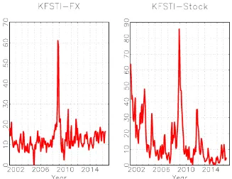
We employ the …nancial stress index (KFSTI) data to quantify the …nancial vul-nerability in Korea. The Bank of Korea introduced the index in 2007 and report KFSTI on a yearly basis in their Financial Stability Report. We obtained monthly frequency data, which in principle are for internal use only.8 The data is available
from May 1995, but our sample period covers from October 2000 until August 2016 to obtain a large panel of predictor variables.
We use the following two KFSTI sub-indices, one for the foreign exchange market (KFSTI-FX) and the other one for the stock market (KFSTI-Stock). We do not report forecasting exercise results for the two other KFSTI sub-indices for the bond market and for the …nancial industry, since our model performed relatively poorly for these two indices. Such limited performances of our factor models might be due to the fact that our common factors are extracted only from macroeconomic variables even though the …nancial industries and bond markets are often in‡uenced by non-economic political factors.
Figure 1 provides graphs of the KFSTI-FX and the KFSTI-Stock. We note that both indices exhibit a sharp spike during the recent …nancial crisis that began in 2008. KFSTI-Stock exhibits more frequent turbulent periods in comparison with dynamics of the KFSTI-FX.
Figure 1 around here
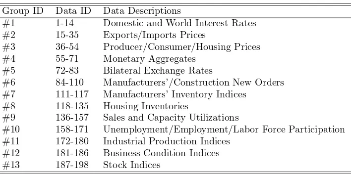
We obtained 198 predictor variables from the Bank of Korea. Observations are monthly frequency and span from October 2000 to August 2016. All variables other than those in percent (e.g., interest rates and unemployment rates) are log-transformed prior to estimations. We categorized these 198 time series data into 13 groups as summarized in Table 1.
Group #1 includes 14 domestic and world nominal interest rates. Groups #2 through #4 are an array of prices and monetary aggregate variables, while group #5 consist of bilateral nominal exchange rates. That is, groups #1 through #5
represent nominal sector variables in Korea. On the other hand, groups #6 through #11 entail various kinds of real activity variables such as production, inventory, and labor market variables. The last two groups represent business condition indices and stock market indices in Korea, respectively.
Table 1 around here
3.2
Evaluations of the Model
This subsection discusses the in-sample …t and the out-of-sample prediction perfor-mance of our PLS factor models relative to those of the benchmark and PC factor models.
3.2.1 In-Sample Fit Analysis
Figure 2 reports estimatedlevel PC factors,^ft=Pt s=2
^f
s, for up to 6 factors, along
with their associated factor loading coe¢cient estimates (^). In Figures 3 and 4, we report level PLS factors ^ct = Pt
s=2 ^cs for the KFSTI-FX and the KFSTI-Stock,
respectively, and their weight matrix estimates (w^). Note that we report two sets
of PLS factors whereas only one set of PC factors is presented. This is because the PLS method utilizes the covariance between the predictor variables and the target variable, whereas the PC method does not consider the target variable when it extracts the common factors.
We noticed that PC factors are very di¤erent from PLS factors for each KF-STI index. Further, we note that ^ estimates are very di¤erent from w^, meaning
that PLS and PC factor estimates are obtained from utilizing di¤erent combina-tions of the predictor variables x. Since we are mainly interested in out-of-sample
predictability performances of the PLS method relative other models, we do not attempt to trace the sources of these factors. However, distinct factor estimates from the PLS and the PC methods imply that the performance of these methods would di¤er in out-of-sample forecasting exercises we report in what follows.
We also reportR2 values in Figure 5, obtained from LS regressions of the target variable yt on estimated factors, ^ctand ^ft, for up to 12 factors. Not surprisingly,
PLS factors provide much better in-sample …t performance than PC factors, because
^ctis estimated using the covariance between the target and the predictor variables.
For example, R2 from ^c1 is over 0.3, whereas that from f^1 is slightly over 0.02
for the KFSTI-FX. In the case of the KFSTI-Stock,R2 from ^c1 is about 0.2, while ^
f1 virtually has no explanatory power.
Note that f^10 and f^2 have the highest R2 for the KFSTI-FX and for the
KFSTI-Stock, respectively, whereas contributions of PLS factors are the highest for the …rst factor estimate ^c1. That is, marginal R2 decreases when we regress
the target variable to the next PLS factors. This is because we extract orthogonal
PLS factors sequentially, utilizing the remaining covariances of the target and the predictor variables. Since the PC method uses only the predictor variables without considering the target variable, marginal R2 values do not necessarily decrease. CumulativeR2value with up to 12 PLS factors is about 0.8 for both indices, whereas that with PC factors is less than 0.3 and 0.2 for the foreign exchange index and the stock index, respectively. In a nutshell, the PLS method yields superior in-sample …t performance in comparison with the PC method.
Figure 5 around here
3.2.2 Out-of-Sample Forecasting Performance
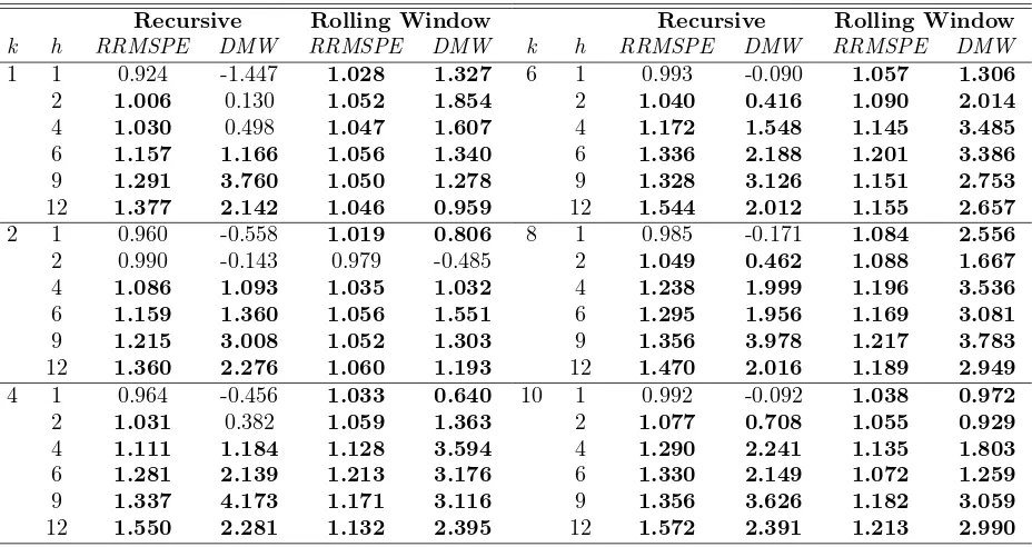
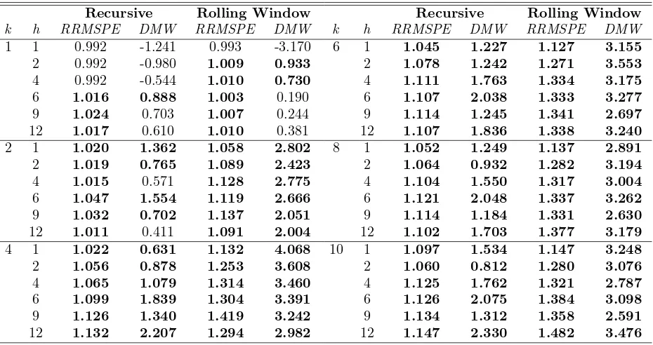
In Tables 2 and 3, we report RRMSPE’s and the DMW statistics of the PLS-RW forecasting model (9) relative to the performance of the PLS-RW benchmark model (11) for the KFSTI-FX and the KFSTI-Stock, respectively. We implement out-of-sample forecast exercises using up to 12 (k) factor estimates obtained from PLS for
fyt+j; xi;tgfor up to 12-month forecast horizons (h). We usedp50% for the sample
split point, that is, initial 50% observations were used to formulate the …rst out-of-sample forecast in implementing forecasting exercises via the recursive (expanding window) scheme as well as the …xed-size rolling window scheme.
consistently outperforms the RW benchmark model in all forecast horizons and in both the recursive and the rolling window method. It should be noted that we use critical values from McCracken (2007) instead of the asymptotic critical values from the standard normal distribution, because the PLS-RW model nests the RW benchmark model.9
Tables 2 and 3 around here
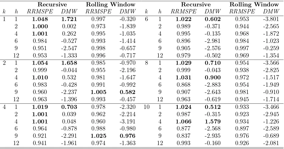
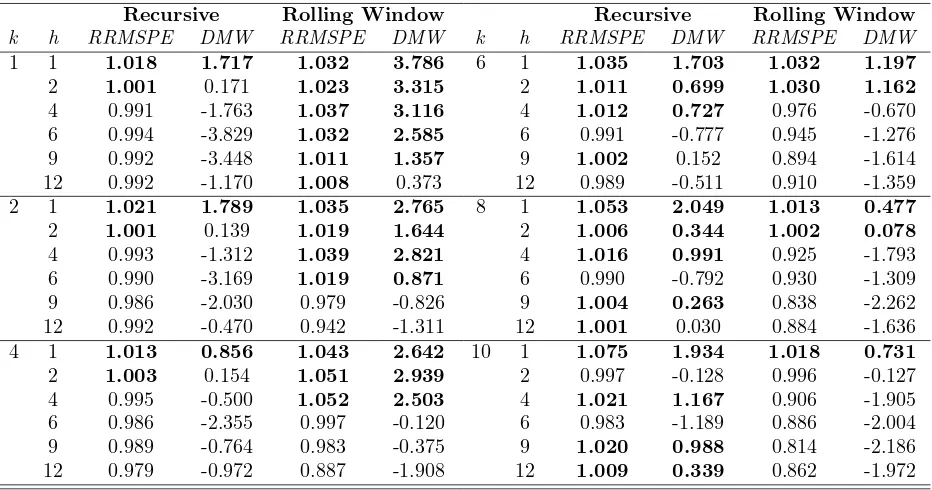
Tables 4 and 5 report the forecasting performance of the PLS-AR model (13) relative to the AR benchmark model (15). Results sharply contrast with earlier results reported in Tables 2 and 3. The PLS-AR model outperforms the AR model only in the short-term forecast horizons. More speci…cally, the PLS-AR model outperforms the AR model in 1-month ahead out-of-sample forecast for the KFSTI-FX under the recursive forecasting scheme, while the AR model performs better in most other cases. The PLS-AR model performs relatively better for the KFSTI-Stock, as RRMSPE values are greater than 1 at least in one-month ahead forecast for the index under the both schemes.
Even though the performance of the PLS-AR model relative to the AR bench-mark is not overwhelmingly good, it should be noted that the PLS-AR model can still provide useful early warning indicators of incoming danger to Korea’s …nan-cial market. Finan…nan-cial crises often occur abruptly and unexpectedly. Given such tendency, it is good to have an instrument that generates warning signs before the systemic risks materialize in the …nancial market.
Tables 4 and 5 around here
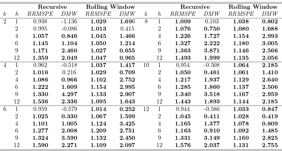
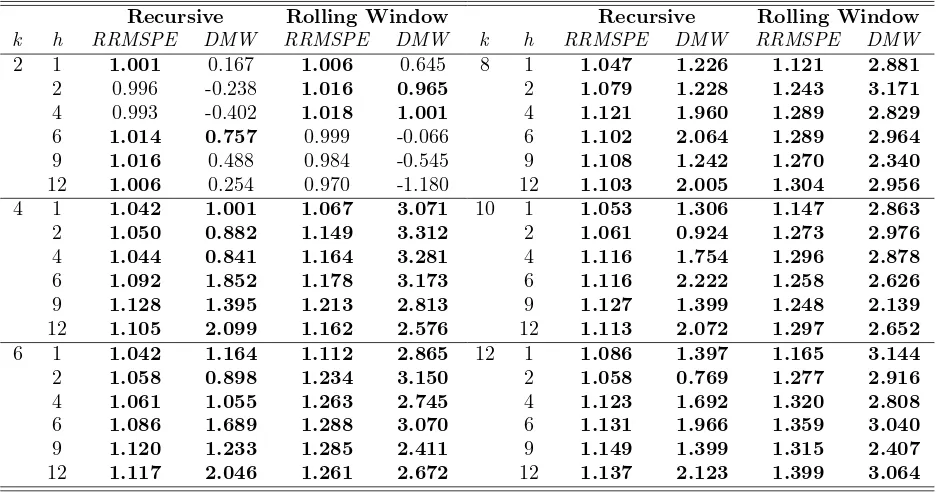
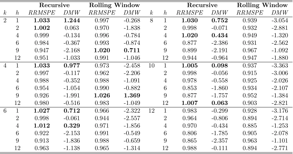
We repeat the same exercises using combinations of ^ct and ^ft and report
the results in Tables 6 through 9. That is, we extended the benchmark forecasting models using equal numbers of factors obtained from the PLS and the PC methods. For example, k = 4 means that c^1, ^c2, f^1, and f^2 are used as condensed
pre-dictor variables. Results are qualitatively similar to previous performances reported
in Tables 2 through 5. That is, marginal contributions of using PC factors ( ^ft) in
addition to PLS factors ( ^ct) are mostly negligibly small.
Tables 6 through 9 around here
3.2.3 Comparisons with the PC Models
This sub-section compares the out-of-sample prediction performances of the PLS models relative to those of the PC models using the RRMSPE criteria, theRMSPE
from the PLS model divided by the RMSPE from the corresponding PC model. That is, RRMSPE greater than 1 implies a better performance of the PLS model.
As can be seen in Figure 6 for the KFSTI-FX, the PLS-RW model outperforms the PC-RW model in all forecast horizons we consider. It is interesting to see that the PLS-RW model’s relative performance becomes better as we employ more factor estimates or when forecast horizons become longer. On the other hand, we observed qualitatively similar performance of the PLS-AR model and the PC-AR model in predicting the KFSTI-FX, even though the PLS-AR model tend to perform better in short-term forecast horizons with many factor estimates.
Figure 6 around here
The PLS-RW model again demonstrates substantially better performance than the PC-RW model in predicting the KFSTI-Stock in all forecast horizons under both the recursive and the …xed-size rolling window schemes. Interestingly, the PC-AR model overall outperforms the PLS-AR model for the KFSTI-Stock under the recursive scheme, while the latter outperforms the former under the …xed-size rolling window scheme. This seems to explain slight improvements in forecasting performance, see Tables 5 and 9, under the recursive scheme when we combine PLS and PC factors together.
Lastly, we compare the performances of the PLS-AR model and the PLS-RW model using theRRMSPE criteria. RRMSPE greater than 1 implies that the PLS-AR model outperforms the PLS-RW model. Results are reported in Figure 8. It should be noted that both PLS models perform similarly well in short-term forecast horizons unless very small numbers of factors are employed. However, as the forecast horizon increases, the PLS-AR model tend to outperform the PLS-RW model. Note that the PLS-RW is based on the RW model, which is a "no change" prediction model. If the KFSTI obeys a mean reverting stochastic process, RW type models would not perform well in long-term forecast horizons. To check this possibility, we employed the conventional ADF test, which rejected the null of nonstationarity at the 5% signi…cance level for both indices, con…rming the conjecture described earlier.10
Figure 8 around here
4
Concluding Remarks
This paper proposes a factor-augmented forecasting model for the systemic risks in Korea’s …nancial markets using the partial least squares (PLS) method as an alterna-tive to the method of the principal components (PC). Unlike PC factor models that estimate common factors solely from predictor variables, the PLS approach gener-ates thetarget speci…c common factors utilizing covariances between the predictors and the target variable.
Taking the Bank of Korea’s Financial Stress Index (KFSTI) as a proxy variable of the …nancial vulnerability in Korea, we applied PLS to a large panel of 198 monthly frequency macroeconomic variables and the KFSTI from October 2000 to June 2016. Obtaining PLS common factors, we augmented the two benchmark models, the random walk (RW) model and the stationary autoregressive (AR) type model, with estimated PLS factors to out-of-sample forecast the KFSTI for the foreign exchange market and the stock market. We then implemented an array of
out-of-sample prediction exercises using the recursive (expanding window) and the …xed-size rolling window schemes for 1-month to 1-year forecast horizons.
References
Andersson, M. (2009): “A Comparison of Nine PLS1 Algorithms,” Journal of Chemometrics, 23, 518–529.
Bai, J., and S. Ng (2004): “A PANIC Attack on Unit Roots and Cointegration,”
Econometrica, 72(4), 1127–1177.
Boivin, J., and S. Ng(2006): “Are more data always better for factor analysis?,”
Journal of Econometrics, 132(1), 169–194.
Christensen, I., and F. Li(2014): “Predicting Financial Stress Events: A Signal
Extraction Approach,” Working Paper 2014-37. Bank of Canada.
Cipollini, A., and G. Kapetanios (2009): “Forecasting Financial Crises and Contagion in Asia using Dynamic Factor Analysis,”Journal of Empirical Finance, 16(2), 188–200.
Edison, H. J.(2003): “Do indicators of …nancial crises work? An evaluation of an early warning system.,” International Journal of Finance and Economics, 8 (1), 11–53.
EI-Shagi, M., T. Knedlik, and G. von Schweinitz (2013): “Predicting
Fi-nancial Crises: The (Statistical) Signi…cance of the Signals Approach,” Journal of International Money and Finance, 35, 75–103.
Eichengreen, B., A. K. Rose, and C. Wyplosz (1995): “Exchange Market
Mayhem: The Antecedents and Aftermath of Speculative Attacks,” Economic Policy, 10 (21), 249–312.
Frankel, J., and G. Saravelos (2012): “Can leading indicators assess coun-try vulnerability? Evidence from the 2008–09 global …nancial crisis,” Journal of International Economics, 87, 216 –231.
Girton, and Roper (1977): “A Monetary Model of Exchange Market Pressure
Applied to the Postwar Canadian Experience,” American Economic Review, 67, 537–548.
Groen, J., and G. Kapetanios (2016): “Revisiting useful approaches to data-rich macroeconomic forecasting,” Computational Statistics and Data Analysis, 100, 221–239.
Helland, I. S.(1990): “Partial Least Squares Regression and Statistical Models,”
Scandinavian Journal of Statistics, 17, 97–114.
Kaminsky, G., S. Lizondo, and C. Reinhart (1998): “Leading indicators of currency crises,” IMF Working Paper No. 45 International Monetary Fund.
Kelly, B., and S. Pruitt (2015): “The three-pass regression …lter: A new ap-proach to forecasting using many predictors,” Journal of Econometrics, 186(2), 294–316.
Kim, H., W. Shi, and H. H. Kim (2016): “Forecasting Financial Stress Indices
in Korea: A Factor Model Approach,” Auburn Economics Working Paper Series auwp2016-10, Department of Economics, Auburn University.
McCracken, M. W. (2007): “Asymptotics for out of sample tests of Granger causality,”Journal of Econometrics, 140, 719–752.
Nelson, C. R., and C. I. Plosser (1982): “Trends and random walks in macro-econmic time series : Some evidence and implications,” Journal of Monetary Economics, 10(2), 139–162.
Oet, M. V., R. Eiben, T. Bianco, D. Gramlich, and S. J. Ong (2011): “The
Financial Stress Index: Identi…cation of System Risk Conditions,” Working Paper No. 1130, Federal Reserve Bank of Cleveland.
Reinhart, C. M., and K. S. Rogoff (2009): This Time Is Di¤erent: Eight Centuries of Financial Folly, vol. 1 of Economics Books. Princeton University Press.
(2014): “Recovery from Financial Crises: Evidence from 100 Episodes,”
Sachs, J., A. Tornell, and A. Velasco(1996): “Financial Crises in Emerging
Markets: The Lessons from 1995,”Brookings Papers on Economic Activity, 27(1), 147–199.
Stock, J. H., and M. W. Watson (2002): “Macroeconomic Forecasting using Di¤usion Indexes,”Journal of Business and Economic Statistics, 20(2), 147–162. Wold, H. (1982): Soft modelling: the basic design and some extensions, vol. 1 of
Table 1. Macroeconomic Data Descriptions
Group ID Data ID Data Descriptions
#1 1-14 Domestic and World Interest Rates
#2 15-35 Exports/Imports Prices
#3 36-54 Producer/Consumer/Housing Prices
#4 55-71 Monetary Aggregates
#5 72-83 Bilateral Exchange Rates
#6 84-110 Manufacturers’/Construction New Orders #7 111-117 Manufacturers’ Inventory Indices
#8 118-135 Housing Inventories
#9 136-157 Sales and Capacity Utilizations
#10 158-171 Unemployment/Employment/Labor Force Participation #11 172-180 Industrial Production Indices
Table 2. PLS-RW vs. RW: Foreign Exchange Market
b
yP LSRW
t+j|t =yt+ˆγ
′
j∆ctvs. byBMt+j|RWt =yt
Recursive Rolling Window Recursive Rolling Window
k h RRMSPE DMW RRMSPE DMW k h RRMSPE DMW RRMSPE DMW
1 1 0.924 -1.447 1.028 1.327 6 1 0.993 -0.090 1.057 1.306
2 1.006 0.130 1.052 1.854 2 1.040 0.416 1.090 2.014
4 1.030 0.498 1.047 1.607 4 1.172 1.548 1.145 3.485
6 1.157 1.166 1.056 1.340 6 1.336 2.188 1.201 3.386
9 1.291 3.760 1.050 1.278 9 1.328 3.126 1.151 2.753
12 1.377 2.142 1.046 0.959 12 1.544 2.012 1.155 2.657
2 1 0.960 -0.558 1.019 0.806 8 1 0.985 -0.171 1.084 2.556
2 0.990 -0.143 0.979 -0.485 2 1.049 0.462 1.088 1.667
4 1.086 1.093 1.035 1.032 4 1.238 1.999 1.196 3.536
6 1.159 1.360 1.056 1.551 6 1.295 1.956 1.169 3.081
9 1.215 3.008 1.052 1.303 9 1.356 3.978 1.217 3.783
12 1.360 2.276 1.060 1.193 12 1.470 2.016 1.189 2.949
4 1 0.964 -0.456 1.033 0.640 10 1 0.992 -0.092 1.038 0.972
2 1.031 0.382 1.059 1.363 2 1.077 0.708 1.055 0.929
4 1.111 1.184 1.128 3.594 4 1.290 2.241 1.135 1.803
6 1.281 2.139 1.213 3.176 6 1.330 2.149 1.072 1.259
9 1.337 4.173 1.171 3.116 9 1.356 3.626 1.182 3.059
12 1.550 2.281 1.132 2.395 12 1.572 2.391 1.213 2.990
Note:RRMSPE denotes the ratio of the root mean squared prediction errors, which is the mean squared prediction
error (RMSPE) from the benchmark model divided by the RMSPE from the competing Partial Least Squares
Table 3. PLS-RW vs. RW: Stock Market
b
yP LSRW
t+j|t =yt+ˆγ
′
j∆ctvs. byBMt+j|RWt =yt
Recursive Rolling Window Recursive Rolling Window
k h RRMSPE DMW RRMSPE DMW k h RRMSPE DMW RRMSPE DMW
1 1 0.992 -1.241 0.993 -3.170 6 1 1.045 1.227 1.127 3.155
2 0.992 -0.980 1.009 0.933 2 1.078 1.242 1.271 3.553
4 0.992 -0.544 1.010 0.730 4 1.111 1.763 1.334 3.175
6 1.016 0.888 1.003 0.190 6 1.107 2.038 1.333 3.277
9 1.024 0.703 1.007 0.244 9 1.114 1.245 1.341 2.697
12 1.017 0.610 1.010 0.381 12 1.107 1.836 1.338 3.240
2 1 1.020 1.362 1.058 2.802 8 1 1.052 1.249 1.137 2.891
2 1.019 0.765 1.089 2.423 2 1.064 0.932 1.282 3.194
4 1.015 0.571 1.128 2.775 4 1.104 1.550 1.317 3.004
6 1.047 1.554 1.119 2.666 6 1.121 2.048 1.337 3.262
9 1.032 0.702 1.137 2.051 9 1.114 1.184 1.331 2.630
12 1.011 0.411 1.091 2.004 12 1.102 1.703 1.377 3.179
4 1 1.022 0.631 1.132 4.068 10 1 1.097 1.534 1.147 3.248
2 1.056 0.878 1.253 3.608 2 1.060 0.812 1.280 3.076
4 1.065 1.079 1.314 3.460 4 1.125 1.762 1.321 2.787
6 1.099 1.839 1.304 3.391 6 1.126 2.075 1.384 3.098
9 1.126 1.340 1.419 3.242 9 1.134 1.312 1.358 2.591
12 1.132 2.207 1.294 2.982 12 1.147 2.330 1.482 3.476
Note:RRMSPE denotes the ratio of the root mean squared prediction errors, which is the mean squared prediction
error (RMSPE) from the benchmark model divided by the RMSPE from the competing Partial Least Squares
Table 4. PLS-AR vs. AR: Foreign Exchange Market
b
yP LSAR
t+j|t = ˆαjyt+βˆ
′
j∆ctvs. bytBM+j|ARt = ˆαjyt
Recursive Rolling Window Recursive Rolling Window
k h RRMSPE DMW RRMSPE DMW k h RRMSPE DMW RRMSPE DMW
1 1 1.048 1.721 0.997 -0.320 6 1 1.022 0.602 0.953 -3.801
2 1.000 0.002 0.973 -1.839 2 0.989 -0.371 0.944 -2.565
4 1.001 0.262 0.995 -1.035 4 0.995 -0.135 0.968 -1.872
6 0.984 -0.527 0.993 -1.414 6 0.896 -2.981 0.984 -1.023
9 0.951 -2.547 0.998 -0.657 9 0.905 -2.576 0.997 -0.259
12 0.953 -1.333 0.996 -0.717 12 0.979 -0.502 0.969 -1.354
2 1 1.054 1.658 0.985 -0.970 8 1 1.029 0.710 0.954 -3.566
2 0.999 -0.044 0.955 -2.196 2 0.999 -0.043 0.938 -2.825
4 1.010 0.532 0.981 -1.647 4 1.031 0.900 0.972 -1.517
6 0.983 -0.428 0.991 -0.992 6 0.868 -2.883 0.954 -1.949
9 0.960 -2.237 1.005 0.582 9 0.907 -2.643 0.981 -0.910
12 0.963 -1.396 0.993 -0.457 12 0.963 -0.619 0.945 -1.714
4 1 1.019 0.703 0.978 -2.320 10 1 1.024 0.512 0.933 -3.466
2 1.001 0.039 0.962 -2.214 2 0.987 -0.315 0.923 -2.945
4 1.001 0.048 0.960 -3.191 4 1.066 1.579 0.934 -1.226
6 0.964 -0.878 0.988 -0.980 6 0.877 -2.568 0.897 -2.589
9 0.921 -2.291 1.025 0.976 9 0.837 -2.935 0.976 -0.689
12 0.941 -1.961 0.974 -1.363 12 0.993 -0.160 0.926 -2.081
Note:RRMSPE denotes the ratio of the root mean squared prediction errors, which is the mean squared prediction
error (RMSPE) from the benchmark model divided by the RMSPE from the competing Partial Least Squares
Table 5. PLS-AR vs. AR: Stock Market
b
yP LSAR
t+j|t = ˆαjyt+βˆ
′
j∆ctvs. bytBM+j|ARt = ˆαjyt
Recursive Rolling Window Recursive Rolling Window
k h RRMSPE DMW RRMSPE DMW k h RRMSPE DMW RRMSPE DMW
1 1 1.018 1.717 1.032 3.786 6 1 1.035 1.703 1.032 1.197
2 1.001 0.171 1.023 3.315 2 1.011 0.699 1.030 1.162
4 0.991 -1.763 1.037 3.116 4 1.012 0.727 0.976 -0.670
6 0.994 -3.829 1.032 2.585 6 0.991 -0.777 0.945 -1.276
9 0.992 -3.448 1.011 1.357 9 1.002 0.152 0.894 -1.614
12 0.992 -1.170 1.008 0.373 12 0.989 -0.511 0.910 -1.359
2 1 1.021 1.789 1.035 2.765 8 1 1.053 2.049 1.013 0.477
2 1.001 0.139 1.019 1.644 2 1.006 0.344 1.002 0.078
4 0.993 -1.312 1.039 2.821 4 1.016 0.991 0.925 -1.793
6 0.990 -3.169 1.019 0.871 6 0.990 -0.792 0.930 -1.309
9 0.986 -2.030 0.979 -0.826 9 1.004 0.263 0.838 -2.262
12 0.992 -0.470 0.942 -1.311 12 1.001 0.030 0.884 -1.636
4 1 1.013 0.856 1.043 2.642 10 1 1.075 1.934 1.018 0.731
2 1.003 0.154 1.051 2.939 2 0.997 -0.128 0.996 -0.127
4 0.995 -0.500 1.052 2.503 4 1.021 1.167 0.906 -1.905
6 0.986 -2.355 0.997 -0.120 6 0.983 -1.189 0.886 -2.004
9 0.989 -0.764 0.983 -0.375 9 1.020 0.988 0.814 -2.186
12 0.979 -0.972 0.887 -1.908 12 1.009 0.339 0.862 -1.972
Note:RRMSPE denotes the ratio of the root mean squared prediction errors, which is the mean squared prediction
error (RMSPE) from the benchmark model divided by the RMSPE from the competing Partial Least Squares
Table 6. PLS-PCA-RW vs. RW: Foreign Exchange Market
b
yP LS/P CRW
t+j|t =yt+ϕˆ
′
j∆ztvs. ybBMt+j|RWt =yt
Recursive Rolling Window Recursive Rolling Window
k h RRMSPE DMW RRMSPE DMW k h RRMSPE DMW RRMSPE DMW
2 1 0.938 -1.136 1.029 1.696 8 1 1.009 0.103 1.038 0.802
2 0.995 -0.086 1.013 0.415 2 1.076 0.750 1.080 1.688
4 1.057 0.846 1.045 1.466 4 1.226 1.727 1.154 2.993
6 1.145 1.104 1.050 1.214 6 1.327 2.222 1.180 3.005
9 1.171 2.460 1.027 0.655 9 1.363 3.871 1.146 2.566
12 1.359 2.049 1.047 0.965 12 1.493 1.999 1.135 2.056
4 1 0.962 -0.518 1.037 1.417 10 1 0.954 -0.508 1.064 2.185
2 1.016 0.216 1.029 0.709 2 1.050 0.461 1.061 1.410
4 1.086 0.966 1.102 2.752 4 1.217 1.937 1.129 2.640
6 1.222 1.609 1.154 2.995 6 1.285 1.860 1.137 2.506
9 1.330 4.297 1.133 2.907 9 1.340 3.518 1.167 2.959
12 1.536 2.336 1.095 1.643 12 1.443 1.893 1.144 2.185
6 1 0.959 -0.579 1.014 0.252 12 1 0.944 -0.586 1.033 0.847
2 1.025 0.330 1.067 1.599 2 1.045 0.411 1.028 0.419
4 1.101 1.005 1.124 3.425 4 1.165 1.377 1.078 0.809
6 1.277 2.008 1.209 2.751 6 1.163 0.910 1.092 1.485
9 1.324 3.590 1.132 2.450 9 1.331 3.149 1.160 2.825
12 1.590 2.271 1.109 2.097 12 1.576 2.037 1.131 2.755
Note:RRMSPE denotes the ratio of the root mean squared prediction errors, which is the mean squared prediction
error (RMSPE) from the benchmark model divided by the RMSPE from the competing Partial Least Squares
Table 7. PLS-PC-RW vs. RW: Stock Market
b
yP LS/P CRW
t+j|t =yt+ϕˆ
′
j∆ztvs. ybBMt+j|RWt =yt
Recursive Rolling Window Recursive Rolling Window
k h RRMSPE DMW RRMSPE DMW k h RRMSPE DMW RRMSPE DMW
2 1 1.001 0.167 1.006 0.645 8 1 1.047 1.226 1.121 2.881
2 0.996 -0.238 1.016 0.965 2 1.079 1.228 1.243 3.171
4 0.993 -0.402 1.018 1.001 4 1.121 1.960 1.289 2.829
6 1.014 0.757 0.999 -0.066 6 1.102 2.064 1.289 2.964
9 1.016 0.488 0.984 -0.545 9 1.108 1.242 1.270 2.340
12 1.006 0.254 0.970 -1.180 12 1.103 2.005 1.304 2.956
4 1 1.042 1.001 1.067 3.071 10 1 1.053 1.306 1.147 2.863
2 1.050 0.882 1.149 3.312 2 1.061 0.924 1.273 2.976
4 1.044 0.841 1.164 3.281 4 1.116 1.754 1.296 2.878
6 1.092 1.852 1.178 3.173 6 1.116 2.222 1.258 2.626
9 1.128 1.395 1.213 2.813 9 1.127 1.399 1.248 2.139
12 1.105 2.099 1.162 2.576 12 1.113 2.072 1.297 2.652
6 1 1.042 1.164 1.112 2.865 12 1 1.086 1.397 1.165 3.144
2 1.058 0.898 1.234 3.150 2 1.058 0.769 1.277 2.916
4 1.061 1.055 1.263 2.745 4 1.123 1.692 1.320 2.808
6 1.086 1.689 1.288 3.070 6 1.131 1.966 1.359 3.040
9 1.120 1.233 1.285 2.411 9 1.149 1.399 1.315 2.407
12 1.117 2.046 1.261 2.672 12 1.137 2.123 1.399 3.064
Note:RRMSPE denotes the ratio of the root mean squared prediction errors, which is the mean squared prediction
error (RMSPE) from the benchmark model divided by the RMSPE from the competing Partial Least Squares
Table 8. PLS-PCA-AR vs. AR: Foreign Exchange Market
b
yP LS/P CAR
t+j|t = ˆαjyt+ˆω
′
j∆zt vs. ybtBM+j|ARt = ˆαjyt
Recursive Rolling Window Recursive Rolling Window
k h RRMSPE DMW RRMSPE DMW k h RRMSPE DMW RRMSPE DMW
2 1 1.033 1.244 0.997 -0.268 8 1 1.030 0.752 0.939 -3.054
2 1.002 0.063 0.970 -1.838 2 0.998 -0.071 0.932 -2.881
4 0.999 -0.134 0.996 -0.784 4 1.020 0.434 0.949 -1.320
6 0.984 -0.367 0.993 -0.874 6 0.877 -2.386 0.931 -2.562
9 0.947 -2.168 1.020 0.711 9 0.899 -2.191 0.967 -1.092
12 0.951 -1.033 0.991 -1.046 12 0.944 -0.964 0.947 -1.880
4 1 1.033 0.977 0.973 -2.458 10 1 1.005 0.098 0.937 -3.363
2 0.997 -0.117 0.962 -2.206 2 0.998 -0.056 0.915 -3.006
4 0.988 -0.352 0.988 -1.091 4 0.978 -0.558 0.925 -2.026
6 0.954 -1.054 0.990 -0.882 6 0.853 -1.860 0.934 -2.107
9 0.926 -1.991 1.026 1.369 9 0.877 -1.757 0.952 -1.384
12 0.980 -0.516 0.983 -1.049 12 1.007 0.063 0.903 -2.821
6 1 1.027 0.712 0.966 -2.322 12 1 0.983 -0.299 0.928 -3.176
2 0.998 -0.061 0.944 -2.557 2 0.964 -0.806 0.894 -2.714
4 1.012 0.329 0.971 -1.856 4 0.970 -0.434 0.885 -1.253
6 0.922 -2.153 0.991 -0.549 6 0.806 -1.785 0.905 -2.078
9 0.913 -1.836 0.988 -0.659 9 0.865 -2.357 0.963 -1.101
12 0.963 -1.138 0.965 -1.314 12 0.988 -0.111 0.894 -2.771
Note:RRMSPE denotes the ratio of the root mean squared prediction errors, which is the mean squared prediction
error (RMSPE) from the benchmark model divided by the RMSPE from the competing Partial Least Squares
Table 9. PLS-PCA-AR vs. AR: Stock Market
b
yP LS/P CAR
t+j|t = ˆαjyt+ˆω
′
j∆zt vs. ybtBM+j|ARt = ˆαjyt
Recursive Rolling Window Recursive Rolling Window
k h RRMSPE DMW RRMSPE DMW k h RRMSPE DMW RRMSPE DMW
2 1 1.021 1.510 1.039 2.691 8 1 1.044 1.733 1.020 0.768
2 1.001 0.135 1.022 1.897 2 1.011 0.609 1.002 0.100
4 0.990 -1.818 1.038 2.722 4 1.021 1.265 0.928 -1.829
6 0.993 -2.431 1.018 0.954 6 0.984 -1.202 0.922 -1.516
9 0.997 -0.349 0.973 -0.886 9 1.019 0.942 0.820 -2.984
12 0.999 -0.091 0.923 -1.604 12 1.018 0.633 0.874 -2.109
4 1 1.033 1.344 1.028 1.901 10 1 1.053 1.936 1.026 0.890
2 1.015 0.782 1.027 2.017 2 1.004 0.234 0.998 -0.049
4 0.999 -0.108 1.015 0.902 4 1.021 1.307 0.917 -1.880
6 1.002 0.242 1.002 0.090 6 0.990 -0.634 0.887 -1.763
9 1.011 0.649 0.957 -1.076 9 1.022 1.009 0.805 -2.280
12 0.991 -0.471 0.916 -1.696 12 1.027 0.914 0.848 -1.750
6 1 1.050 2.068 1.016 0.702 12 1 1.069 1.729 1.034 1.189
2 1.010 0.485 1.019 0.775 2 0.999 -0.062 0.993 -0.183
4 1.001 0.056 0.953 -1.359 4 1.020 1.069 0.906 -1.853
6 0.993 -0.784 0.918 -2.330 6 0.999 -0.081 0.887 -1.884
9 1.015 1.191 0.846 -2.666 9 1.047 1.846 0.809 -2.298
12 0.996 -0.191 0.869 -2.200 12 1.024 0.832 0.848 -1.903
Note:RRMSPE denotes the ratio of the root mean squared prediction errors, which is the mean squared prediction
error (RMSPE) from the benchmark model divided by the RMSPE from the competing Partial Least Squares
Figure 2. Principal Component Analysis
Figure 3. Partial Least Squares Estimation: Foreign Exchange Market
Figure 4. Partial Least Squares Estimation: Stock Market
Figure 5. In-Sample Fit Analysis: R Squares
Figure 6. Cross-Comparisons: Foreign Exchange Market
Figure 7. Cross-Comparisons: Stock Market
Note: We report theRRMSPE defined as theRMSPE of the PC method divided theRMSPE of the PLS. That
Figure 8. Cross-Comparisons: PLS-RW vs. PLS-AR
Note: We report theRRMSPE defined as theRMSPE of the PLS-RW model divided theRMSPE of the PLS-AR