Comments Concerning Some Features of Phase Diagrams and Phase Transformations

Comments Concerning Some Features of Phase Diagrams

and Phase Transformations

Thaddeus B. Massalski

Materials Science and Engineering, and Physics, Carnegie-Mellon University, Pittsburgh, PA, USA

Several interesting features in the study of stabilities of phases, and in phase transformations, are discussed. It is proposed that symmetry considerations related to the presence of magnetism in iron suggests that the respective phases, BCC alpha and FCC gamma, have in fact lower symmetries than cubic. A proposal is made that the symbol beta used in the past for the designation of the paramagnetic BCC iron should perhaps be returned as a feature in phase diagrams. The importance of the new concept of a ‘pseudogap’ in the electronic band structure, as a stabilizing electronic feature, is discussed in the light of the Hume-Rothery electron concentration rule. It is proposed that since the thermal activation is a major feature in the behavior of isothermal martensites, a more suitable designation for these types of phase transformations might be ‘‘thermally activated martensites’’, or TAMs. Massive transformations are discussed briefly and it is emphasized that they present a specific example of an idiomorphic transformation process, not requiring the need for orientation relationships (ORs) between the parent and product phases.

[doi:10.2320/matertrans.M2010012]

(Received January 12, 2010; Accepted January 29, 2010; Published March 17, 2010)

Keywords: phase stability, phase transformation, Fe, Hume-Rothery electron concentration rule, pseudogap, martensites, massive transformations

1. Phase Diagrams and Phase Stability

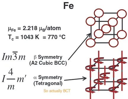
1.1 Symmetry and the structure of phases — Should we return thephase to the Fe phase diagram? In terms of conventional crystallography, the structure of a phase may be defined as a result of positioning of a ‘‘motif’’ of atoms (or groups of atoms) upon a ‘‘lattice’’ of points in space. Difficulties arise when we begin to apply this concept to motifs that are more complicated than just neutral single atoms. I will illustrate this with reference to the elements iron (Fe) and plutonium (Pu), which exhibit allotropic structure changes depending on temperature. The sequence of allo-tropic phases in Fe includes the phase, as was considered to be the case in the late 1800’s and early 1900’s. This was based mainly upon the work of Roberts-Austen,1)_{but was put} into question later by many authors2–4)_{when the structures of} the,andphases were determined by X-ray diffraction to be all BCC.5)

The difference between the and phases involves the change in magnetism: phase is ferromagnetic below the Curie temperature, andphase is paramagnetic above. In the late 1920’s and 1930’s the phase was abandoned in published phase diagrams mainly because X-ray diffraction seemed unable to reveal any change of structure. However, one may correctly argue that there is a change of symmetry, from tetragonal to cubic, and that this constitutes a phase change. Recently, D.E. Laughlin and I have argued this point in a contribution to the Ricardo Ferro Symposium.6) _We proposed to adopt a definition of a phase that includes order parameters specifying additional properties to be considered in addition to the composition and structure; such parameters as atomic order, magnetic order, electronic configuration, etc. This enlarged definition of a phase can already be found earlier in the writings of Landau,7)or Christian,8)and others.

As illustrated in Fig. 1, the overall symmetry is lowered when the motif of ordered magnetic moments is included. The repetition of lattice (points) and the motif of the atoms with aligned magnetic moments reduce a plane group symmetry of4mmto a plane group symmetry of2mmonly by a change in the motif, not the lattice. As a consequence, if all such moments are aligned in one direction on a bcc lattice, say along the [001] direction, they create an overall direc-tional motif that changes the structure. Some people would say that even if the cubic lattice retains the symmetry of the crystal parameters (a¼b¼c), the total spatial symmetry of the structure is nevertheless lowered from Im33m to I4

mm 0_,

due to the aligned moments. Arguments of this kind have been used for several years now by Laughlin et al.9) and others10–15) to discuss the symmetry of crystals that have magnetic moments associated with the atoms. So, the motif can change the lattice. That is a tricky statement, but there are plenty of comments on this now in the literature. Some people may say, I will accept this concept if the presence

Fe

µµFe= 2.218 µB/atom Tc= 1043 K = 770 °C

Im

3

m

I

4

m

m

Symmetry (A2 Cubic BCC)

Symmetry (Tetragonal)

So actually BCT

Fig. 1 The BCC crystal structure, including magnetic and symmetry information.9)

*_{The Fifty-Fifth Gold Medalist of the Japan Institute of Metals, 2010}

Emeritus Professor, Carnegie-Melon University E-mail: [email protected]

of the BCT structure is demonstrated experimentally, even if it cannot be demonstrated by X-ray diffraction. Perhaps measurements of magnetostriction can accomplish this.16) Numerous features of magnetic materials, such as magnetic domains, domain interactions, magnetocrystaline anisotropy, and magnetostriction, can be addressed more accurately by starting with the full symmetry aspects of the magnetic state, i.e. the structure with reduced symmetry due to the magnetic ordering rather than the original cubic lattice. Electronic structure calculations for such materials produce more consistent results when the symmetry is reduced due to the ordered magnetic state. Accurate orbital magnetic moments of BCC iron can only be obtained from calculations that introduce a lowering of the symmetry, from 48 (cubic) to 16 (tetragonal) operations, resulting from the preferred orienta-tion of the magnetic spin moments along the [001] easy axis. Cubic symmetry does not support ferromagnetism because the aligned moments always favor a special direction. So, as more ‘‘ground state’’ calculations are becoming involved in assessment of phase stability, perhaps the time has come to accept these subtle features of crystal structure.

Although not cubic, PrCo5 has yielded experimental

evidence of symmetry reduction upon magnetic ordering. Shen and Laughlin17) _{have shown by convergent beam} electron diffraction that the projected point group symmetry along the [0001] direction of PrCo5is reduced from6mmto

6 on magnetic ordering. This implies that the space group changes from P6/mmm in the paramagnetic state to P6/ mm0m0in the ferromagnetic state. Equally interesting are the calculations by Widom and Mihalkovic,18) regarding the crystal structure of boron. Experimental work suggests that the -rhombohedral (black) form is stable over all temper-atures from 0 K to melting. However, early calculations indicate that its energy is larger than the energy of the -rhombohedral (red) form, implying that the phase cannot be stable at low temperatures. Furthermore, the form exhibits partially occupied sites, seemingly in conflict with the thermodynamic requirement that entropy vanishes at the low temperatures (the Third Law). Using electronic density functional methods, Widom and Mihalkovic conclude that this unique, energy-minimizing pattern of occupied and vacant sites can be stable at low temperatures, but this seems to break the-rhombohedral symmetry.

Returning to the general question regarding the sequence of phases in Fe, as depicted at present in phase diagrams and accepted in books,2–4)_{should we restore thesymbol to the} phase diagram? My personal preference is yes, but perhaps another solution would be to call the presentphase as0_, and the phase above the Curie temperature as, similarly to the situation with the atomic order transition (0_{to) in the} case of the Cu-Znbrass.

Later on I shall remind you that at very low temperatures the (metastable) FCC gamma phase of Fe may also be regarded as tetragonal. When gamma becomes antiferro-magnetic (AF) below the Neel temperature (TN), gamma AF may in fact be regarded as no longer cubic, but FCT in this new phase nomenclature context. One can ask—is the ferromagnetic FCC Ni also actually FCT? Laughlin suggests that it is actually rhombohedral, because the magnetic moments are aligned in the [111] direction.

Perhaps I should also mention that in the case of other elements that exhibit numerous allotropic changes, there are similar arguments about symmetry, namely, that the acceptance of the existence of additional ‘‘order parameters’’ (magnetic, electronic, etc.) affecting the motif in the definition of a ‘‘phase’’ tends to reduce the crystal structure symmetry. We can start with a ‘‘cubic lattice’’, but if we add to it a motif (for example a non-symmetric distribution of the electronic bonding forces which show directional features) the resulting ‘‘structure’’ can be regarded as having a ‘‘lower symmetry’’. For example, in Pu the sequence of phases is

!!!!0_{!"!liquid. The X-ray studies} show that the structure is FCC. It can be argued, however,19,20) that Pu atoms in the Pu phase are not all electronically the same, and may exhibit ‘‘lattice position dependence’’ indicated by the fact that the calculated bonding forces between them vary strikingly and are highly uniso-tropic, depending on the location on the FCC lattice. There is still an additional difficulty here, namely the fact that first principles calculations are ‘‘ground state’’ calculations (at 0 K) and the actual structure exists at much higher temperatures.

The picture of bonding forces between atoms in Pu, as illustrated in Fig. 2, suggests that Pu is totally different from a classical FCC metal, like Al, where all forces between atoms are the same,19,20) and where the structure is indis-putably A2. So, here again, the total symmetry of the Pu

phase may be considered to be reduced from FCC to c-centered monoclinic, if the arguments based on the first principles calculations for 0 K are accepted.

1.2 Competition for stability between the allotropic phases in Fe: — Is the occurrence of antiferromag-netism at very low temperatures in the gamma phase of Fe responsible for the observed BCC>FCC>

BCC transition?

As is well known, the role of magnetism in deciding the competition for stability between the observed allotropic changes with temperature in Fe can be considered in terms of the usual thermodynamic Gibbs free energies:

Gi¼HiTSi ð1Þ

whereirefers to either phaseor phase. Similarly, both enthalpy and entropy are expressed as

Hi¼Hi₀þ

ZT

T0

Ci_PdT ð2Þ

and

Si¼Si₀þ

ZT

T0

C_Pi

T dT; ð3Þ

whereCi

Prepresents the specific heat at constant pressure for the phase i,T0 is 0 K andH0i is the enthalpy at 0 K. Thus,

eq. (1) is explicitly rewritten as

Gi¼H₀iþ

ZT

T0

C_PidTT

ZT

T0

Ci_P

Keeping in mind the Third Law,21)the entropyS0of a pure

element is zero at 0 K. Thus, we see that the Gibbs free energy can be expressed in terms of the specific heats Cp, which can be measured experimentally, or evaluated from a suitable model:22,24,25)

CP¼3R E

T

2

eE=T

ðeE=T1Þ2

þaTþbT4þC_Pmag; ð5Þ

where the first term represents the Einstein specific heat with the Einstein temperatureE, the second term the electronic specific heat, the third term anharmonic lattice specific heat and the last term magnetic specific heat.

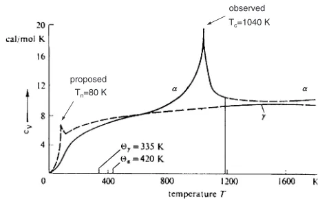
In the case of Fe, it is still a relatively little known fact that at very low temperatures the FCC form of iron, i.e., the , metastable, but retained artificially2,23)is antiferromagnetic (AF). This is also confirmed by the observed1=trend with temperature in thephase which, when extrapolated to 0 K, cuts the temperature axis at a negative value. So, we may expect a Neel peak at low temperatures in the corresponding

specific heat trend. Similarly, a Curie peak due to the ferromagnetic/paramagnetic transition at higher tempera-tures in the BCC (i.e. the) form of Fe at 770_{C (1043 K) is} a well documented feature in the measured specific heats. These trends are shown in Fig. 3, which is from Haasen’s book.23)_{The Neel temperature is indicated as a small peak,} but it has not been studied in detail experimentally. A recent calculation22) _{places the T}

N at 67 K. The actual Cp data collected together for both phases is shown in Fig. 4.24)

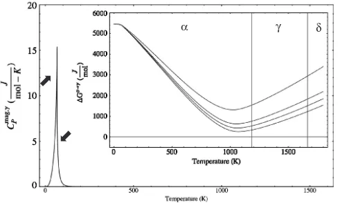
Recently, we have modeled the competition for phase stability as a function of temperature between the and

forms of Fe by examining the effect of the magnetic peaks on the respective free energies of these phases and the resulting difference in the Gibbs free energy, G!_{. For the Neel}

peak in we introduced small changes in both the position and the shape of the peak, and for the Curie peak in, where the temperature of the peak is well established, we introduced only small changes of shape compatible with the observed experimental data. Figures 5 and 6 show the results of such modeling.24)

The situation may be considered as follows: Starting at 0 K, when the respective entropies of both phases may be assumed to be zero, the enthaply H<H because the

magnetic interaction in the ferromagneticis stronger than the interaction in the antiferromagnetic . As already mentioned, as temperature rises, the free energy of each phase is related to the specific heat (Fig. 3). A little aboveTN, the paramagnetic phase will be even less stable compared to the (still ferromagnetic), but at higher temperatures the situation begins to change when the negative entropy terms (TS), each related to the respective specific heat, increas-ingly come into play in the free energy of each phase. The modeling confirms that at the well documented phase transition temperature of 911_{C (1184 K), theG}! _value

becomes negative, as expected, but only by a very small amount. This indicates that it must be the Gibbs energy reduction in the gamma phase due the Neel peak at low temperatures, and the relatedTSterm, that tips the balance. At still higher temperatures the BCC structure returns in the form of the delta phase at 1393_{C (1666 K), when the} vibrational entropy effect in the ‘more open’ BCC structure imparts to it a comparable advantage. Thus, it can be argued that if the FCC were not AF at low temperatures, there

Pu

Fig. 2 Two stacked fcc unit cells with the central atom showing the 12 nearest neighbours. In the case of plutonium, the 12 bonds with the nearest neighbours widely vary with strength and can be separated into six pairs: blue (3.3), black (3.5–3.7), red (3.7–3.9), pink (3.9–4.1), green (4.5–4.7) and brown (4.7–5.3). When the fcc lattice is combined with the motif of these bond strengths, the resultant space group is monoclinic Cm.19)

observed

proposed Tn=80 K

Tc=1040 K

α α

would be insufficient free energy reduction for it to be stable at high temperatures when it is paramagnetic. Perhaps there is also an additional contribution to the specific heats of gamma iron from lattice harmonics, as argued some years ago by Zener.25) _{We should also be aware that T}

N is likely to be a function of experimental details (dispersed particle sizes, stresses, matrix influences etc.), so until the magnitude of the Neel peak, its shape and form, as well as the exact temperatureTN, are well established experimentally, or the whole low temperature range modeled in still more detail, the above conclusion involves a certain degree of speculation. Our modeling indicates that raising the TN by just a few degrees higher than 67 K eliminates the gamma phase altogether.

1.3 Hume-Rothery electron concentration rule and band calculations for structurally complex alloys: — What is the current status of the H-R electron concentration rule?

At a recent Symposium honoring the scientific contribu-tions of William Hume-Rothery and their links to current research, I attempted to single out which are the most important rules Hume-Rothery proposed many years ago when discussing alloy phase stability. It seems that three rules, related to the atom size effects, the electrochemical effects, and the electron concentration effects, are likely to continue to be regarded as the ‘‘Hume-Rothery Rules’’.26) Undoubtedly, the electron concentration rule amongst the three has earned the greatest recognition in the field of materials science as a simple and useful guide for designing and understanding alloying behavior. As illustrated in Fig. 7, this rule established in the early 1930’s, showed that Fig. 4 Temperature dependence of experimentally measured specific heats of iron.24)

α γ δ

Fig. 5 Modeled height and shape changes of the Neel peak in the specific heats of gamma iron at low temperatures, and their effect on the related Gibbs free energies. The arrow on the left of the peak indicates height changes, and the one on the right indicates shape changes of the peak. The insert indicates the resulting changes in the Gibbs free energy difference

G!_{as a function of temperature between theandforms of Fe.}24)

T_N= 67K TN= 70K T_N= 75K T_N= 80K T_N= 85K

T = 1184K T = 1665K

Fig. 6 Modeled changes in the Gibbs free energy difference G!

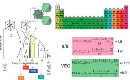
successively appearing-,-,-,"- andphases in the phase diagrams based on the noble metals, Cu, Ag and Au, can be scaled with respect to the number of average electron concentration per atom,e=a, regardless of the atomic species of the polyvalent element involved as the alloying partner with a given noble metal. Among such ‘‘electron phases’’, the

-brass phase contains as many as 52 atoms per unit cell, as illustrated in Fig. 7, and can be regarded as being structurally the most complex. It was the subject of intense studies with the X-ray powder diffraction methods by Westgren and Phragme´n in Sweden in the 1920’s, and they were the first to draw attention to the electron concentration significance of the ‘famous’ 21/13 electron to atom ratio.27) Also at about the same time, Hume-Rothery in England similarly emphasized the stabilizing electron concentration role in alloy phases and the value for the -brasses to be e=a¼

21=13¼1:615, characteristic of the two typical stoichio-metric formulas in copper based alloys, Cu5Zn8and Cu9Al4,

which he considered as being compound-like (for a more detailed historical account of these developments please see Ref. 28)).

However, one can express the electron concentration in two ways. One is thee=aas mentioned above, and the other is the VEC, more recently referred to as the valence electron concentration, where all the electrons which are counted include also the d-electrons (and other electrons) accommo-dated in the valence band. The Hume-Rothery Rule obvi-ously does not work if the VEC is used as an electron concentration parameter as shown in Fig. 7. Mizutani has made very significant contributions to clarify and resolve this situation in recent years.28)

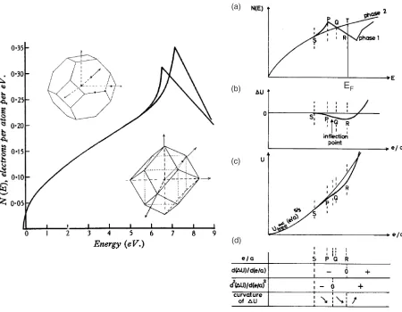
In the 1930’s, Mott and Jones29) interpreted the Hume-Rotherye=arule on the basis of a free electron model of the Fermi surface interacting with the Brillouin zones of different crystal structures ase=achanges. This has come to be known as the Fermi surface-Brillouin zone interaction, FsBz. In 1937, Jones30)_{further attempted to elucidate why the FCC} -phase terminates at e=a¼1:4 and is replaced by the BCC

-phase stable neare=a¼1:5, in the Cu-X binary systems (X¼Zn, Al, Ga, etc.) by using the density of state curves (DOS) as shown in Fig. 8. In this interpretation, the Cu-3d band was not considered, and the van-Hove singularity peaks were those of the FCC-Cu and BCC-Cu. As is well known, this interpretation has run into problems when Pippard demonstrated in 195731)that the Fermi surface of pure copper (i.e. at e=a¼1:0), already makes contact with the {111} zone planes of the Brillouin zone of the face-centered cubic lattice. It was this situation which stimulated a few years later my colleague from Japan, Professor Uichiro Mizutani (working with me in the USA) to review the whole field of Hume-Rothery ‘‘electron phases’’ and to embark on many experimental studies seeking connections between the e=a and the DOS.32,33)

Let me return to Fig. 8 to mention another important contribution due to Jones (1962) regarding phase stability.34) In this work Jones discussed the phase competition in terms of the DOS curves, each characterized by a van-Hove singularity near the Fermi level relative to the free-electron-like monotonic DOS. He stressed the fact that the relative stability of an alloy phase will be enhanced if the DOS curve involves a large peak followed by a subsequently rapidly declining slope, like that in Fig. 8, while that of the

ZnII CdII AlIII GaIII SnIV 1

CuI AgI AuI

3/2

7/4 1.4

21/13

Hume-Rothery Phases

e

/

a

(

Cu

Zn

)

=

1 5

+

2 8

13

=

21

13

e

/

a

(

Cu

Al

)

=

1 9

+

3 4

13

=

21

13

VEC

(

Cu

Zn

)

=

11 5

+

12 8

13

=

151

13

VEC

(

Cu

Al

)

=

11 9

+

3 4

13

=

111

13

e/a

VEC

=11.62

=8.54

=1.61

=1.61

competing phase remains fairly monotonic in a given e=a range. This is illustrated in a sequence shown in Fig. 8(a) to (d) reproduced from an earlier review article mentioned above.32) _{The DOS in phase 1 increases above the free} electron-like parabolic DOS because of the approach of the Fermi surface toward the Brillouin zone (portion SP in Fig. 8(a)), and then decreases following its contact at the pointP(portionPR). At pointR, areasSPQandQRTbecome equal and hence the energies at the Fermi level are the same, E1 ¼E2. The differenceUreaches its largest value atRand

theUversuse=acurve shows a minimum, which is to the right ofPon the energy scale. It is important to realize that the minimum in the energy difference curve is reached not at the contact point for the Fermi surface atP, but at the pointR on the decreasing slope of the DOS curve past the peak. This little-noticed argument (published in France) suggests that Jones implicitly proposed to shift the position of the Fermi level optimal for phase stability to be nearer to the minimum in the DOS in Fig. 8(a) to reach the optimal lowering of the electronic energy of a given structure. In the more recent terminology, this is really equivalent to locating the Fermi level on a declining slope of DOS projecting towards the bottom of a valence band ‘‘pseudogap’’, a concept that has become increasingly the basis of alloy phase stability discussions of more complex Hume-Rothery structures.28)

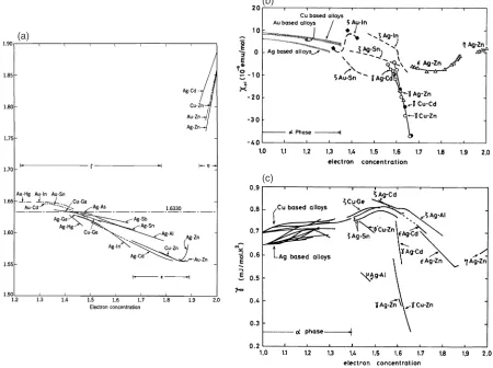
As often happens, significant additional experimental contributions preceded and guided the later theoretical

developments and progress in this field. In the 1960’s, Massalski and King33) _{initiated systematic studies of the} numerous close-packed hexagonal phases (the phases) in the alloy systems of the noble metals, which Hume-Rothery had not considered in his originale=arule. They have shown for the first time that the lattice constants and the axial ratio of these phases exhibit a systematic behavior when plotted against e=a. Their data are reproduced in Fig. 9(a). They interpreted thee=a-dependent lattice constants and the axial ratio trends in terms of the FsBz interaction and claimed that this interaction is the deciding factor that governs the electronic properties and the stability of the phases. So, these phases are also the Hume-Rothery ‘‘electron phases’’. Subsequently, measurements of physical properties even more directly relevant to the electronic structure, such as the magnetic susceptibility, Fig. 9(b), and the electronic specific heat coefficient, Fig. 9(c), have shown a universal e=a dependence for numerous Hume-Rothery phases.32) _In particular, the fact that the DOS-related data for a series of

-brass alloys falls on a rapidly declining universal curve, and are strongly negative in sign, can be taken as evidence for the manifestation of the FsBz interactions associated with {411} and {330} Brillouin zone planes, which form a ‘‘nearly spherical’’ Brillouin zone, as shown in Fig. 10. Massalski and Mizutani32)reviewed all such experimental data in 1978 and pointed out the clear evidence for the influence of the FsBz interactions scaling to the electron concentration, e=a, and

(a)

(b)

(c)

(d)

E_F

Fig. 8 DOS derived from the model of Jones for FCC- and BCC-Cu.30)_{(a)–(d) Schematic illustration of the model of Jones (II) for}

contributing to phase stability. Of most interest, however, is the situation with the-brass structures. Here, the composi-tion ranges where the gamma-brasses are stable, are expected to be located on a sharply declining slope of the DOS for the

-brass because the zone is nearly spherical. In this way, the electronic energy would be most profoundly affected when the Fermi level eventually falls inside a pseudogap. It is interesting to note that this interpretation was made without referring to the word ‘‘pseudogap’’ at that time.32)

Studies and calculations of the electronic features of the

-brass structures, and extensions of electron concentration considerations to the new fields of quasi-crystals and their approximants, have opened a new wide area for testing the Hume-Rothery concepts of the e=a rule. Following the discovery of an Al-Mn quasicrystal by Shechtman et al.in 1984,35)_{Tsaiet al.}36,37)_{discovered a series of thermally stable} quasicrystals in Al-Cu-TM (TM¼Fe, Ru, Os) and Al-Pd-TM (Al-Pd-TM¼Mn and Re) systems over 1988 to 1991 by using the Hume-Rothery electron concentration rule as a guide. They assigned negative valencies to transition metal con-stituent elements, as proposed by Raynor,38)_{and pointed out} that new quasicrystals could be synthesized by searching for alloys, whose average valency falls into e=a values in the vicinity of 1.8. Their works certainly stimulated both metallurgists and physicists not only to search further for new quasicrystals but also to re-examine the physics behind the Hume-Rothery electron concentration rule.

Fujiwara39)_{revealed a depression (i.e., a pseudogap) in the} DOS across the Fermi level by performing the LMTO-ASA first-principles band calculations for the Al-Mn approximant containing 138 atoms in its unit cell, and suggested that this contributes to the stabilization of a quasicrystal. More recently, Mizutani and his collaborators28,40,41) _developed an elegant technique, i.e. the FLAPW-Fourier method to extract the FsBz interactions essential in interpreting the Hume-Rothery electron concentration rule by making use of the fact that the FLAPW wave function outside the muffin-tin sphere is expanded into plane waves with respect to the reciprocal lattice vector allowed for a given lattice.

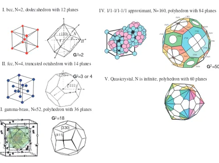
Figure 10 illustrates how an increase in the number of atoms in the unit cell accompanies an increase in the number of the Brillouin zone planes (or the number of relevant equivalent lattice planes), making the Brillouin zone ‘‘more spherical’’. This, in turn, increases the number of directions in the reciprocal space, along which an interference with electrons near the Fermi level takes place and stationary waves are formed. Hence, the larger the number of atoms per unit cell, the deeper is a pseudogap formed at the Fermi level, and the more efficient is the lowering of the electronic energy tending to stabilize a given structure. Among structurally complex alloy phases, Mizutani and his coworkers have studied numerous -brasses, because the-brass is complex enough to produce a sizeable pseudogap at the Fermi level but is still simple

(a)

(b)

(c)

enough to perform the FLAPW band calculations with an efficient speed.28,40,41)

As shown in Fig. 11, the-brasses like Cu5Zn8 with the

space group I443m are formed by arranging the 26-atom clusters to form the BCC lattice, while those like Cu9Al4with

the space groupP443mare formed by arranging two different 26-atom clusters to form the CsCl-like structure. Both Cu5Zn8 and Cu9Al4 compounds contain 52 atoms per unit

cell and are perfectly ordered without any chemical disorder, providing a unique opportunity to perform the first-principles band calculations. The electronic structure for both the Cu5Zn8and Cu9Al4-brasses was calculated by means of the

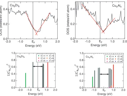
first-principles FLAPW band calculations.28,40)As shown in Fig. 12, the DOSs for both compounds are well characterized by a deep pseudogap across the Fermi level. The energy spectrum of the FLAPW-Fourier components at the principal symmetry point N is shown in the lower panel of Fig. 12 for both compounds over the energy range covering the pseudogap. The electronic states at the bottom and top of the pseudogap are found to be exclusively dominated by the

jGj2¼18 states (i.e. the nearly spherical Brillouin zone), which are apparently split into bonding and antibonding states across the Fermi level due to the interference of electrons with the set of {330} and {411} lattice planes. This is taken as the demonstration of the formation of a FsBz-induced pseudogap associated with the jGj2¼18 in both compounds.

In the most recent monograph about to be published, Mizutani28) _{has emphasized that in order to elucidate the}

physics behind the Hume-Rothery e=arule the problem of assessing the electronic contributions to phase stability can be best approached by calculating the ground state energies via the first-principles band calculations. However, as I mentioned earlier, in such calculations it is necessary to use the VEC as an electron concentration parameter to include all the electrons involved. So, a new challenge has appeared, namely, how to extract from such theoretical calculations the electron concentration parameter e=a that is critically important in assessing the Hume-Rothery electron concen-tration rule. However, since the FLAPW-Fourier method

can be extended to construct a dispersion relation for electrons outside the muffin tin sphere, this can provide a measure of the effective Fermi diameter and, in turn, an effective e=afor the application of the Hume-Rothery rule. Such a dispersion plot is referred to by Mizutani as a Hume-Rothery plot.28,41) _{It confirms that both the Cu}

5Zn8 and

Cu9Al4 gamma-brasses can be assigned the value of e=a

equal to 1.61. This resolves the problem mentioned earlier of usinge=aas a parameter in the Hume-Rothery rule, and using VEC as a parameter in the first-principles band calculations. The above approach also made it possible to derive a new set of effective e=a values for the transition metal elements in the periodic table. They turn out to be slightly positive numbers across the 3d-series. From the point of view of basic theory, these values can be regarded as more sound than the negative valencies developed by Raynor in 1949.38)The newly establishede=avalues can be coupled with the VEC and used to design new functional

V. Quasicrystal, N is infinite, polyhedron with 60 planes

{110} N H P

I. bcc, N=2, dodecahedron with 12 planes

G2₌₂

{002}

{111}

II. fcc, N=4, truncated octahedron with 14 planes

G2_{=3 or 4}

III. gamma-brass, N=52, polyhedron with 36 planes

{411} {330}

G2₌₁₈

(710) (710)

(710) (710) (550)

(550) (550)

(550) (543)

(543)

(543)

(543) (543)

(543)

(543) (543) (543)

(543)

(543) (543)

(543) (543)

(543) (710)

(543)

(543)

IV. 1/1-1/1-1/1 approximant, N=160, polyhedron with 84 planes

G2₌₅₀

alloys and compounds.28) Future research will judge their effectiveness.

My purpose in this section was to attract your attention to the fact that a substantial progress has been achieved in connecting older ideas in materials science to new

develop-ments in physics. It is remarkable how many of the extensions of the Hume-Rothery electron concentration concepts, and particularly their emergence as guiding principles for the understanding and discovery of numerous complex alloy structures, have been developed in Japan.

(

I

43

m

)

(a) Cu

Zn

(b) Cu

Al

(

P

43

m

)

IT (Cu) OT (Cu) OH (Cu) CO (Al) IT (Al)

OT (Cu) OH (Cu) CO (Cu) IT (Zn)

OT (Cu) OH (Cu) CO (Zn)

cluster “a” cluster “b”

Fig. 11 26-atom cluster in (a) Cu5Zn8and (b) Cu9Al4gamma-brasses with space groupsI443mandP443m, respectively.28)

1.0

0.8

0.6

0.4

0.2

0.0

Σ|

C

i Ghkl

/2

|

2

-2.0 -1.0 1.0 2.0

Energy (eV)

G2=14 G2=18 G2=22 G2=26 G2=30 G2=34

Cu₅Zn₈

E_F

1.0

0.8

0.6

0.4

0.2

0.0

Σ

|

C

i Ghkl

/2

|

2

-2.0 -1.0 1.0 2.0

Energy (eV) G2=14 G2=18 G2=22 G2=26 G2=30 G2=34

Cu₉Al₄

E_F

0.4

0.2

0.0

DOS (states/eV.atom)

-2.0 -1.0 1.0 2.0

Energy (eV) E_F Cu₅Zn₈

0.4

0.2

0.0

DOS (states/eV.atom)

-2.0 -1.0 1.0 2.0

Energy (eV) E_F

Cu₉Al₄

Fig. 12 (top panel) DOS for for Cu5Zn8and Cu9Al4gamma-brasses. A red line is drawn as guide to eye to envisage the presence of a

pseudogap across the Fermi level. (bottom panel) Energy spectrum of the FLAPW-Fourier components of the FLAPW wave function outside the muffin-tin sphere at the principal symmetry pointNin the neighborhood of the Fermi level for Cu5Zn8and Cu9Al4

2. Phase Transformations

The area of Phase Transformations has been of great interest at different times in my research career. The field of phase transformations is also very large, like the field of phase diagrams, and many attempts have been made to classify transformations. Professor Jack Christian, my pred-ecessor JIM gold medal winner, has made well known contributions here. Today, I would like to comment on two specific types of transformations. In the displacive (non-diffusional) phase transformations group, there is a subgroup sometimes referred to as ‘‘isothermal martensites’’, and in the diffusional transformation group there is a subgroup known as the ‘‘massive transformations’’ (which I happen to have named more than 50 years ago42,43)). So, I will make a few observations on both of these small subgroups.

2.1 Isothermal Martensitic Transformations: — Is ther-mally activated martensite (TAM) a better term than isothermal martensite (IM)?

There is a very large literature on the isothermal martensitic transformations, including much work in Japan. Experimental work in this field typically involves kinetic studies, or structural studies, during cooling and reheating, with only a few experiments actually performed ‘‘at constant temperature’’. I will comment only on the terminology, the kinetics and the activation features of isothermal martensites. Recently, there was a symposium in the USA on phase transformations, just published this year.44)

The kinetics of martensitic phase transformations are usually designated as being either athermal or isothermal.

Athermalimplies that the transformation is not (hence theA)

thermally activated, i.e., in an athermal transformation there is no thermal activation necessary for the transformation to proceed. Athermal transformations therefore do not depend ontimebut depend on the change in temperature. The word

isothermal (the same heat) is used as an adjective for a transformation that occurs at a constant (same) temperature. When used in the context of martensitic transformations, isothermal refers to those transformations that proceed with time and are therefore contrasted withathermal transforma-tionswhich require cooling or heating to proceed, and are not thermally activated.45–47)It is helpful to realize that the term

thermaldescribes different concepts in the words isothermal

and athermal. In isothermal,thermalimplies ‘‘temperature’’, while in athermal, thermal is short for ‘‘not thermally activated’’.45)

Although the literature contrastsisothermalwithathermal, not all non-athermal transformations are necessarily thermal. There may be thermally activated processes which occur on continuous cooling. These have sometimes been called

anisothermal48) _{but the term is rarely used. In martensite} which forms athermally, thermal energy is insufficient to initiate the transformation. Whatever the mechanism of the initiation of the transformation is, it cannot proceed by thermally influenced fluctuations. The athermal transforma-tion is initiated at specific sites only after a large enough chemical driving force is generated by cooling to a large enough degree below the equilibrium phase transformation temperature. This thermodynamic driving force must

over-come the elastic (plastic) energy which is in opposition to the initiation of the transformation at specific sites and at below Ms. Thermal activation implies a statistical probability, meaning the same site will not always be repeatedly the first one to initiate the process. This is unlike in some of the

thermoelastic martensites where the same site has been shown to repeatedly initiate the process.49)

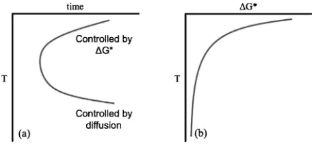
Since the isothermal martensites involve time as a major parameter, theT-T-T(transformation-time-temperature) dia-grams have been used to depict the progress of a given transformation. The well known C-curve shape for the isothermal thermal activated precipitation reactions can be plotted on aTTT diagram as shown in Fig. 13. The time to form the new phase initially decreases as the temperature is lowered below the equilibrium transformation temperature, due to the decrease in the barrier to nucleation, G, as shown in Fig. 13. This decrease in the nucleation barrier occurs because the thermodynamic driving force increases as the material is cooled to lower temperatures. However the time to form the new phase begins to increase at lower temperatures due to the lack of thermal energy necessary for diffusion to take place. In terms of the thermally activated processes, nucleation controls the upper region of the C-curve while diffusion controls the lower region of the C-curve. The C-curve behavior on TTT diagrams depicting the thermally activated martensitic transformations (see Fig. 14) cannot be explained in the same way as precipitation transformations because there is little or no activation barrier to growth in thermally activated martensitic transformations. Of course all thermally activated processes must cease at 0 K, but the TTT curves for the thermally activated martensitic transformations bend back well above 0 K. Thus, it appears that the barrier to nucleation must also have the shape of a C-curve if it controls the transformation kinetics. Since this barrier has within it the elastic energy of the transformation, such an increase in the barrier can arise because of an increase in the elastic stiffness of the matrix at lower temperatures. This has been discussed by Lobodyuk and Estrin.50)

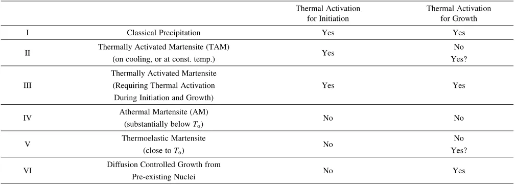
Laughlin et al.45) _{have considered some possibilities} regarding the role of thermal activation and summarize them in the form of Table 1, where I have also included the thermoelastic martensites for comparison. We suggested that the isothermal martensites could be conveniently renamed as thermally activated martensites (or TAMs).45) The TAMs have thermal activation only at the initiation stage, because Fig. 13 Schematic of (a) a typicalTTTcurve for a diffusion controlled precipitation transformation and (b) a plot of G_{, the barrier to}

the subsequent growth stage normally occurs rapidly, and in a martensitic mode, without requiring thermal activation. Of course there could be TAMs which have thermal activation in their initiation process, as well as in their growth process. These also would show a C-curve behavior and would be difficult to distinguish from the normally observed ‘‘iso-thermal martensites’’.

In contrast, athermal martensitic transformations exhibit no activated processes and they do not need waiting time (incubation) to proceed, only a sufficient thermodynamic driving force obtained by lowering the temperature. A fifth possibility is also included in the table, namely one in which the initiation stage does not require thermal activation, but the growth stage does. This would also be the case for diffusion controlled precipitation reactions that grow from pre-existing nuclei. As pointed out by Laughlinet al.45)_and also by Linet al.,51)_{it is of interest to note that there could} occur sequences of martensitic transformations as shown in Table 2. These sequences can also be illustrated on theTTT diagrams.

As is well known, the majority of TAMs are studied during continuous cooling, or during cooling and subsequent holding at temperature. In Fig. 14 are shown progressions of different types of possible martensitic transformations. The relative position of theMsand the nose of the TAM

C-curve, and the rate of cooling allows for several possible sequences of transformations. In Fig. 15(a), the Ms temper-ature for athermal martensite has been placed above the knee of theTTTcurve, but below the highest temperature at which TAM can form, Msi.45,52) Cooling curve 1 represents the sequence of an athermal martensitic transformation followed by a TAM. In contrast to this, curves 2 and 3 represent transformations which proceed from athermal to anisother-mal to isotheranisother-mal. This is because the isotheranisother-mal hold temperature was not reached before the material passed through the TTT curve, allowing for some thermally activated process to occur during the continuous cooling stage before the isothermal martensite begins to form.50)

Figure 15(b) shows aTTTcurve in which theMs temper-ature is below the knee of theTTTcurve.45)Cooling curve 4 Table 1 Thermal activation of phase transformation processes.

Thermal Activation for Initiation

Thermal Activation for Growth

I Classical Precipitation Yes Yes

II Thermally Activated Martensite (TAM) Yes No

(on cooling, or at const. temp.) Yes?

Thermally Activated Martensite

III (Requiring Thermal Activation Yes Yes

During Initiation and Growth)

IV Athermal Martensite (AM) No No

(substantially belowTo)

V Thermoelastic Martensite No No

(close toTo) Yes?

VI Diffusion Controlled Growth from No Yes

Pre-existing Nuclei

Table 2 Possible martensitic transformation sequences.

Isothermal

Athermal!Isothermal

Anisothermal!Isothermal

Athermal!Anisothermal!Isothermal

Anisothermal!Athermal!Isothermal

‘‘Mixed Athermal and Anisothermal’’!Isothermal

Fig. 15 Schematic of the possible sequence of different martensitic transformations with (a)Ms above and (b) below the nose of theTTT

Curve.45)

Fig. 14 Schematic of (a) a typicalTTT curve for a thermally activated martensitic transformation and (b) a plot of the smallestG_{for the given}

represents an overall transformation which starts as athermal one and after holding at a temperature below the Ms, and below the knee of the curve becomes isothermal in character. Curve 5 shows a transformation which starts as an aniso-thermal one, becomes aaniso-thermal belowMs, but when held at a constant temperature belowMsand below the C curve knee, it becomes isothermal in character. Curve 6 represents a transformation which begins anisothermally and becomes isothermal on holding at a constant temperature above Ms. Finally, curve 7 represents an isothermal martenstitic trans-formation at a constant temperature. After holding at this temperature an athermal reaction could develop on further cooling below Ms, depending on how far the TAM has progressed.

So, since the isothermal martensite is a thermally activated martensite, perhaps the term isothermal martensite should be replaced with the more descriptive and more accurate term TAM. One can consider further possibilities if the C-curve for TAMs is displaced more to the left, eventually intersect-ing the temperature (T) axis. The transformation will then appear to be an athermal one since it occurs rapidly without any apparent incubation time. Such a transformation could be called a ‘‘pseudo-athermal’’ transformation. One way to distinguish this kind of transformation from a truly athermal transformation is to hold the sample at the temperature at which the transformation was first observed. If it does not proceed with time it is truly an athermal transformation. If, however, the transformation continues over an extended period of time it is seen to be thermally activated and hence it started as an anisothermal transformation. For more details see Refs. 44) and 45).

2.2 Massive Transformations: Can totally idiomorphic nucleation and growth occur in diffusional trans-formations?

Massive transformations have been studied since the late 1950’s,42) and the actual definition of this type of trans-formation is still a matter of some discussion. However, in my brief comments today I would like to address mainly the crystallographic features and not the kinetics of this trans-formation process. One of the main questions regarding

massive transformations has been whether or not there is a crystallographic orientation relationship between the parent phase and the product phase as the massive grains nucleate and grow. Such orientation relationships are almost always observed in diffusional transformations, and they are ex-pected on the basis of activation energy arguments in the theory of transformations.

itself and not of the matrix as shown in Figs. 18(a) and (b). Many years ago, Prof. C. S. Smith56)_{has suggested a parent/} product interface possibility as shown in Figs. 19, and also in the schematic picture in Fig. 16. Recent HRTEM pictures confirm this possibility when the nucleation appears to take place at the parent phase boundary (Figs. 20(a) and (b)). However, during subsequent growth the idiomorphic feature is clearly seen in the HRTEM micrographs, confirming the existence of the type-3 (incoherent and irrational) interfa-ces.57)_{Faceting is frequently observed along such incoherent} interfaces (for detailed references see Refs. 47) and 48)). In view of these recent symposia and discussions the most appropriate definition of a typical massive transformation seems to be best defined as follows: ‘‘a composition-invariant, interface-controlled diffusional phase transforma-tion, involving a characteristic patchy microstructure and frequent faceting and ledges, but not necessarily involving lattice orientation relationships’’.43)A suitable name for the idiomorphic massive phase product has not been established. So, these various forms of massive transformations continue being studied with increasingly sophisticated techniques and present a real challenge to researchers, also

in Japan where the massive transformation has been studied very little. The overall conclusion at present is that

isomorphic massive transformations are a specific unique feature and that there can be diffusional transformations that show no orientation relationships, i.e. no communication between parent and product phases, both in the nucleation and growth stages.

Acknowledgments

My friends in Japan know well that in my long research career I have been involved in many diverse topics in the wide field of Materials Science. In this presentation, I have touched on just a few subjects that may be currently of interest, and with which I have had a personal connection. This also enables me to mention a few scientific dilemmas and controversies. Since this is an invited lecture I have written it in ‘first person’ style.

I wish to express many thanks to my colleagues Professor Uichiro Mizutani in Japan and Professor David Laughlin in the USA for many stimulating discussions and for their help in the preparation of this manuscript.

Fig. 17 Lack of orientation relationships (ORs) between matrix and massive grains in a partial massive transformation in a Cu-Zn alloy, as demonstrated by X-ray selective area diffraction.43)

Fig. 18 (a) HREM image of a curved section of an"-interface and (b) higher magnification of selected area showing composite (020) andf111gnanofacets/terraces/ledges.55)

Fig. 19 (a) Classical critical nucleus model for singly faceted grain boundary nucleus which is incoherent with respect to grain2but coherent

or semi-coherent with respect to1. (b) Grain boundary nucleus involving

REFERENCES

1) S. W. Smith:Roberts-Austen: A record of his works, (Charles-Griffin and Company, Limited: London, 1914) pp. 18–25.

2) C. S. Barrett and T. B. Massalski:The Structure of Metals, (McGraw-Hill, New York, 1966).

3) S. Epstein:The Alloys of Iron and Carbon, Volume 1: Constitution, (McGraw-Hill, New York, 1936).

4) T. Nishizawa: Thermodynamics of Microstructures, (ASM Interna-tional, Materials Park, Ohio, 2008).

5) A. Westgren and G. Phragme´n: J. Iron Steel Inst.105(1922) 241. 6) T. B. Massalski and D. E. Laughlin: Calphad33(2009) 3.

7) L. D. Laudau and E. M. Lifshitz:Statistical Physics, (Pergamon Press, New York, 1980).

8) J. W. Christian:The Theory of Transformations in Metals and Alloys, Part I, (Pergamon Press, New York, 1975).

9) D. E. Laughlin, M. A. Willard and M. E. McHenry: Magnetic Ordering: Some Structural Aspects. Phase Transformations and Evolution in Materials, ed. by P. Turchi and A. Gonis, (The Minerals, Metals and Materials Society, Warrendale, 2000) pp. 121–137. 10) W. Opechowski and R. Guccione:Magnetic Symmetry, in Magnetism

IIA ed. by G. T. Rado and H. Shul (Academic Press, New York, 1965). 11) B. K. Vainshtein:Modern Crystallography I, (Springer-Verlag, 1981). 12) A. P. Cracknell:Magnetism in Crystalline Materials, (Pergamon Press,

New York, 1975).

13) S. Shaskolskaya:Fundamentals of Crystal Physics, Chapter VIII (Mir Publishers, Moscow, 1982).

14) L. A. Shuvalov:Modern Crystallography IV, (Springer-Verlag, Belin, 1988).

15) S. J. Joshua:Symmetry Principles and Magnetic Symmetry in Solid State Physics, (Adam Hilger, Bristol, 1991).

16) A. P. Cracknell:Magnetism in Crystalline Materials, (Pergamon Press, New York, 1975).

17) Y. Shen and D. E. Laughlin: Phil. Mag. Lett.62(1990) 187. 18) M. Widom and M. Mihalkovic: Phys. Rev. B77(2008) 064113. 19) A. J. Schwartz, H. Cynn, K. J. M. Blobaum, M. A. Wall, K. T. Moore,

W. J. Evans, D. L. Farber, J. R. Jeffries and T. B. Massalski: Prog. Mater. Sci.54(2009) 909.

20) K. T. Moore, D. E. Laughlin, P. So¨nderlind and A. J. Schwartz: Phil. Mag.87(2007) 2571.

21) J. P. Abriata and D. E. Laughlin: Prog. Mater. Sci.49(2004) 367. 22) Q. Chen and B. Sundman: J. Phase Equilibria22(2001) 631. 23) P. Haasen: Physical Metallurgy, (Cambridge University Press,

Cambridge, 1978).

24) T. B. Massalski, D. E. Laughlin and N. Jones: (2010) to be published. 25) C. Zener:Phase Stability In Metals and Alloys, ed. by P. S. Rudman

et al., (McGraw Hill, New York, 1967).

26) T. B. Massalski:The Science of Alloys for the 21st Century: A Hume-Rothery Symposium Celebration, ed. by P. E. A. Turchi, R. D. Shull and A. Gonis, (The Minerals, Metals and Materials Society, Warrendale, 2000) pp. 55–70.

27) A. F. Westgren and G. Phragme´n: Metallwirtschaft7(1928) 700. 28) U. Mizutani: Hume-Rothery rules for structurally complex alloy

phases, (Taylor-Francis, 2010).

29) N. F. Mott and H. Jones:The Theory of the Properties of Metals and Alloys, (Clarendon Press, Oxford, 1936; Dover 1958).

30) H. Jones: Proc. Phys. Soc. A49(1937) 250. 31) A. B. Pippard: Phil. Trans. R. Soc. A250(1957) 325.

32) T. B. Massalski and U. Mizutani: Prog. Mater. Sci.22(1978) 151. 33) T. B. Massalski and W. B. King: Prog. Mater. Sci.10(1961) 1. 34) H. Jones: Journal de Physique et le radium, Paris23(1962) 637. 35) D. Shechtman, I. Blech, D. Gratias and J. W. Cahn: Phys. Rev. Lett.53

(1984) 1951.

36) A. P. Tsai, A. Inoue and T. Masumoto: Jpn. J. Appl. Phys.27(1988) L1587.

37) Y. Yokoyama, A. P. Tsai, A. Inoue, T. Masumoto and H. S. Chen: Mater. Trans. JIM32(1991) 421–428.

38) G. V. Raynor: Prog. Metal Phys.1(1949) 1. 39) T. Fujiwara: Phys. Rev. B40(1989) 942.

40) R. Asahi, H. Sato, T. Takeuchi and U. Mizutani: Phys. Rev. B 71

(2005) 165103.

41) U. Mizutani, R. Asahi, H. Sato and T. Takeuchi: Phys. Rev. B 74

(2006) 235119.

42) T. B. Massalski: Acta Metall.6(1958) 243. 43) T. B. Massalski: Met. Trans.33A(2002) 2277.

44) Santa Fe Symposium, ICOMAT 2008 Santa Fe, New Mexico, USA, (2010) to be published.

45) D. E. Laughlin, N. J. Jones, A. J. Schwartz and T. B. Massalski: Thermally Activated Martensite: Its Relationship To Nonthermally Activated (Athermal) Martensite, ICOMAT 2008 (To be published). 46) L. Kaufman and M. Cohen: Prog. Metal Phys.7(1958) 165. 47) F. J. Pe´rez-Reche, E. Vives, L. Man˜osa and A. Planes: Phys. Rev. Lett.

87(2001) 195701-1.

48) S. C. Das Gupta and B. S. Lement: J. Metals Trans. AIME3(1951) 727. 49) H. Pops and T. B. Massalski: Trans. AIME230(1964) 1662. 50) V. A. Lobodyuk and E. I. Estrin: Phys. Uspekhi48(2005) 713. 51) M. Lin, G. B. Olson and M. Cohen: Metall. Trans. A23A(1992) 2987. 52) Y. Imai and M. Izumiyama: Sci. Rep. Res. Ins. Tohoku University A17

(1965) 135.

53) J. W. Christian:Encyclopedia of Materials Science and Engineering, ed. by M. B. Bever (Pergamon Press, London, 1986) p. 3496. 54) Symposium on Mechanisms of the Massive Transformations, Edited

by H. Aaronson and V. Vasudevan (Met. Trans.33A, No. 8 August (2002)).

55) T. B. Massalski, D. E. Laughlin and W. A. Soffa: Met. Trans.37A

(2006) 825.

56) C. S. Smith: Trans ASM45(1953) 533.

57) P. Li, J. M. Howe and W. T. Reynolds: Met. Trans.37A(2006) 895. Fig. 20 (a) Grain boundary nucleation and growth of L1o-phase in