The implementation of collision avoiding haptic feedback
in the pedal-based control of a robotic platform
S.D. (Sierd) Meijer
B
Sc Report
Committee:
Dr. Ir. D. Dresscher
Dr.ir. E.C. Dertien
August 2018
028RAM2018
Robotics and Mechatronics
EE-Math-CS
University of Twente
Summary
i-Botics aims to improve the knowledge and technology concerning telerobotics and ex-oskeletons. The overarching project of this thesis is about telerobotics, which is a combi-nation of telepresence and teleoperation. This thesis focusses on the improvement of the teleoperation. Teleoperation is about the control of a robot over long distances.
This thesis is about the implementation of haptic feedback in the pedal based control control of a robot. The haptic feedback is supposed to indicate the location of obstacles in the path of motion, reducing the required mental effort to operate the robot. The main goal is divided in three sub goals.
1. A research on different haptic feedback implementations;
2. The design and implementation of a haptic feedback capable interface for the pedals; 3. The implementation of a connection between the pedals’ interface and the robot.
In the analysis an initial plan for the design and implementation phase is set up. First, three kinds of haptic feedback are researched and compared based on their implemen-tation in the system in question. Second, an overview of the existing hardware is made. Third, a controller with a variable spring constant for the pedals is designed. And last, the software architecture and functionality for the whole system is designed.
In the design and implementation chapter, the final implementation is described. The chapter is divided in three sections: electrical, digital and mechanical. Any alterations or additions with respect to the analysis are mention here.
After the final implementation, the system is tested and evaluated. The testing is divided into two parts. The first part tests the pedals’ sensors and the controller, and the second part tests the haptic feedback implementation. All implemented parts are tested individ-ually.
The testing showed that the controller is usable, based on the input from the sensors. The controller is also capable of maintaining a relatively stable state while altering the spring constant. The controller does show unexpected behaviour caused by the delay in the con-troller design. The pedals can operate a virtual robot based on their relative position. The haptic feedback implementation is also tested in a virtual environment and works as ex-pected.
Samenvatting
i-Botics richt zich op het vergroten van de kennis en verbeteren van de technologie op het gebied van telerobotica and exoskeletten. Het overkoepelende project van deze the-sis houdt zich bezig met telerobotica, wat bestaat uit tele-aanwezigheid en tele-operatie. Deze thesis focust op het verbeteren van tele-operatie: het besturen van een robot over lange afstanden.
Deze thesis beschrijft de implementatie van haptische feedback in een pedaal-gestuurde robot. De haptische feedback moet de bestuurder informeren over de locatie en afstand van obstakels op het pad van de robot. De implementatie zou de vereiste mentale inspan-ning voor het besturen van de robot af moeten nemen.
Het hoofddoel bestaat uit drie subdoelen:
1. Het vinden van een geschikte implementatie van haptische feedback;
2. Het ontwerpen en implementeren van een, haptische feedback capabele, interface voor de pedalen;
3. Het implementeren van een verbinding tussen de interface van de pedalen en de robot.
In de analyse is een initieel plan voor de ontwerp- en implementatie-fase opgesteld. Eest zijn drie verschillende soorten haptische feedback onderzocht en vergeleken op basis van hun implementatie in de pedalen. Vervolgens is alle bestaande hardware in kaart ge-bracht. Als derde is een controller met een variabele veerconstante ontworpen. En als laatste is de software architectuur en functionaliteit voor het gehele systeem ontworpen.
In het hoofstuk Ontwerp en Implementatie is de uiteindelijke implementatie besproken. Dit hoofdstuk is verdeeld in drie delen: elektrisch, digitaal en mechanisch. Ook de afwi-jkingen en aanvullingen ten opzichte van de analyse worden hier besproken.
Na de voltooide implementatie is het systeem getest en geëvalueerd. De tests zijn opgedeeld in twee delen. Het eerste deel test de sensoren en de controller van de pedalen. Het tweede deel test de implementatie van de haptische feedback. Alle geïmplementeerde onderdelen zijn individueel getest.
Uit de testen bleek dat, op basis van de sensor waarden, de controller functioneel was. Ook bleef de controller relatief stabiel wanneer de veerconstante veranderde van waarde. De controller vertoonde soms onverwachts gedrag vanwege de vertraging in het ontwerp. De pedalen kunnen een virtuele robot aansturen op basis van de relative positie. De hap-tische feedback is ook getest in een virtuele omgeving en gedroeg zich als verwacht.
Contents
1 Introduction 1
1.1 Context . . . 1
1.2 Project goal . . . 1
1.3 Method . . . 1
1.4 Report outline . . . 1
2 Analysis 3 2.1 Comparing haptic feedback implementations . . . 3
2.2 Hardware . . . 11
2.3 Pedal controller . . . 18
2.4 Software architecture . . . 28
3 Design & implementation 34 3.1 Electrical . . . 35
3.2 Software . . . 38
3.3 Mechanical . . . 47
4 Testing & results 48 4.1 Pedal tests . . . 48
4.2 Simulations . . . 69
5 Conclusion 76 6 Recommendations 78 6.1 Software delay . . . 78
6.2 Controller . . . 78
6.3 Pedal construction . . . 79
1 Introduction
1.1 Context
This assignment is commissioned by i-Botics, a collaboration between TNO and Univer-sity of Twente, and is part of an overarching project aimed at the innovation of teler-obotics. Telerobotics is concerned with the remote control of semi-autonomous robots, in which telepresence and teleoperation is combined. The robot that is used is shown in figure 1.1a and consists of two RMP omni 50 systems that form the base. Attached to the robot is a KUKA LWR 4+ arm with at the end a ReFlex TakkTile gripper. Figure 1.1b shows the Leo Universal Cockpit that is used to operate the robot and is capable of providing the operator video, audio and haptic feedback. The goal of this assignment consists of two parts. The first part is creating an interface between the pedals located in the cockpit and the control of the robot, and the second part is providing the operator with haptic feedback via the pedals.
1.2 Project goal
The goal of this project is to reduce the mental effort required for the control of the robot because during the operation the operator will be mostly focussed on the control of the arm and less so on the control of the robot. Therefore the use of the pedals should be intuitive. This intuitiveness will also be attempted by providing the operator information on the location and distance to obstacles detected by the robot via haptic feedback in the pedals. The haptic feedback should be of a guiding nature to decrease the operators required attention, while not restricting any movability of the platform.
1.3 Method
First, the pedals are equipped with an encoder, accelerometer and motor and need to be connected to an embedded computer running a control system for the operation of the pedals. A connection needs to be established between the embedded computer and ROS (Robotic Operating System), a middleware which is used for the control of the robot. After the pedals are connected to ROS, an algorithm will be implemented for controlling the motion of the robot which is based on the sensors located in the pedal. When full control of the robot is established another algorithm has to be designed for the implementation of haptic feedback. The haptic feedback will be based on the distance and relative location of an obstacle detected by the robot, and the velocity of the robot.
1.4 Report outline
haptic feedback. After the analysis, (chapter 3) the design & implementation is described, which is divided in a hardware and a software part. When the system is fully operational it will be tested based on the project goals set out in the introduction in chapter 4, test-ing & results. Then, a conclusion (chapter 5) is written based on the findtest-ings durtest-ing the assignment and after, recommendations (chapter 6) will be made for future work.
(a) Robotic platform (b) Leo Universal Cockpit
2 Analysis
In the analysis four different aspects of the research question are elaborated upon. First, different kinds of haptic feedback implementations are discussed and how they trans-late into bitrans-lateral pedal control. Second, an overview of the existing hardware is made, whether they will be used and if so, the characteristics they have. Third, the interfacing of the pedals is discussed for both the hardware and the software. And last, the use of ROS is discussed in combination with the results of the hardware and software chosen in the previous part. A simplified overview of the end system is given in figure 2.1.
Figure 2.1: Simplified system overview
2.1 Comparing haptic feedback implementations
There are multiple variations on the implementation of haptic feedback based on obstacle detection. In this section three different implementations are compared and evaluated whether they could be effective in pedal based control. All three implementations have a trade-off between an increase in physical effort and a decrease in mental effort for the operation of the platform. The implementations are force offset, stiffness feedback and force-stiffness feedback.
2.1.1 Force offset
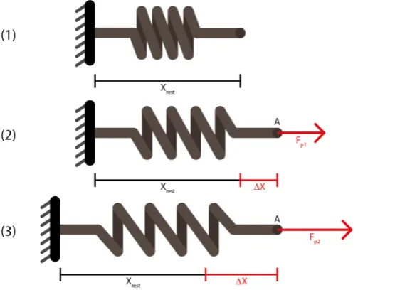
Force offset [1] gives feedback by increasing the position error of the controller based on the distance to an obstacle. This can be compared to a spring of which a supposedly static connection changes in position. Figure 2.2 (1) shows a spring attached to a wall with rest lengthxr est and spring constantKs. Based on Hooke’s law shown in formula 2.1
the exerted force by the spring is 0 because the displacement of the spring is equal to the rest length.
Fspr i ng=Ks·(xr est−x) (2.1)
is required to keep point A in place when an offset is implemented. This force is exerted until it reaches its new rest position.
Figure 2.2: Force offset example (1) Spring at rest length. (2) Spring extended by forceFp1.
(3) Spring influenced by force offset, increasing∆xand forceFp2to keep point A in place
Implementing force offset can inform the operator of the obstacle distance and location without input from the operator, but increases the required physical effort while operat-ing. [2] and [1], [3] show that a force offset improves the collision avoidance when imple-mented with a correct feedback loop gain by shifting the origin positition of the control device so that a collision is avoided if the operator does not give input. A characteristic of force offset feedback is that the offset is also present if no force is exerted by the oper-ator (passive feedback) [1], which means that the way op operating is changed. This can be useful if the controlled platform can move independently, for example an UAV drifting because of wind because the platform will correct itself without input. The distance to an obstacle is inversely proportional to the shift of the origin position giving a good represen-tation of distance when there is no input forc. However, after the offset is compensated the spring constant does not change, and the steering looses its indication of distance. Also important is that the offset needs to be compensated, whenever the operator wants to go straight while in the vicinity of an obstacle a force is required, which increases the required mental effort of the operator instead of decreasing it as shown by [3], [1], [4]. The goal of the implementation of haptic feedback is to assist the operator with maneuvering the platform which should decrease the required mental effort.
based controls have the origin position of the pedal in its most upright position (e.g. car pedals), in this case a force offset would be impossible, however the control of the ped-als in relation to the platform is not definitive yet. Second, the force offset is ped-also present when there is no input force, this was proven to be useful in case of a drifting UAV. How-ever, when implemented in a platform that is unlikely to move because of the friction with the ground, it can lead to the platform moving itself without the input of an operator. This exceeds the role of guiding the operator in controlling the platform. Because the force off-set requires the operator to actively counter the force offoff-set and alters the controls, it is unsuited to be implemented in the pedal based control.
2.1.2 Stiffness feedback
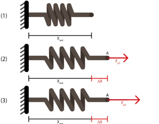
Stiffness feedback [1] alters the spring constant of the controller based on the distance to an obstacle. Controllers that return to their origin position when there is no input force have a physical or virtual spring to do so. Force applied to the virtual spring needs to be larger than the retracting force that the spring exerts in order to extend the spring. Stiffness feedback changes the required force to extend the spring by altering the spring constant as shown by [1], this isKs in formula 2.1. Figure 2.3 (1) again shows a spring
[image:13.595.168.448.394.612.2]at rest length. Figure 2.3 (2) shows a spring with a displacement∆xbecause of a pulling forceFp1. In figure 2.3 (3)Ks is increased which results in a largerFp2in order to keep point A in place.
Figure 2.3: Stiffness feedback example (1) Spring at rest length. (2) Spring extended by forceFp1. (3) Spring influenced by increased spring constantKs, increasingFp2to keep point A in place.
location of an obstacle in rest position, but provides this info while force is exerted on the pedal. The closer an obstacle gets, the more force the pedal will exert on the operator to get to its origin position. This increases the required physical effort, but less than the force offset because there is no constant force required to keep the pedal in its place. One characteristic is that the pedal does not provide any information when there is no force applied to the pedals like the force offset does. A second characteristic is that, because the spring constant is proportional to the distance and the pedal position, there is a rel-atively small feedback force when the operator applies a small force. [1], [3] discuss that this relatively small force could be too small to perceive, which defeats its purpose. [1] do show that in case of a joystick controlled UAV, stiffness feedback results in better per-formance and reduced required mental effort compared to an offset force. Based on the requirements of the system discussed in the introduction, it is beneficial that the pedal does not provide a feedback force when the operator does not apply force because it does not alter the control of the system. The proportional relation between obstacle distance and increased spring constant can be changed into, for example, an exponential function that provides larger force variations when the obstacle is at minimum range.
Applying the stiffness feedback on the pedal based control is a viable option because of its guiding nature. That stiffness feedback does not provide any feedback when there is no force applied, is an advantage because it decreases the required mental effort of the oper-ator. The stiffness feedback does not alter the control, only increases the required physical effort, and thus does not exceed its guiding purpose, making it an option for testing.
2.1.3 Force-stiffness feedback
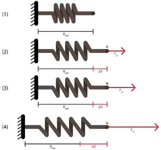
Force offset and stiffness feedback both have their advantages and disadvantages and can be combined into force-stiffness feedback [3]. Force-stiffness feedback combines the ad-vantages of both force offset and stiffness feedback by increasing the force to return to a shifted origin position, based on the distance to an object [2]. [3] explains it as adding force feedback to compensate the small feedback force that is generated by stiffness feed-back when there is a small displacement in the pedal’s position. This is done by adding force directly with an offset force and indirectly by creating a larger distance to the ori-gin, increasing the stiffness feedback force. Equation 2.2 is an adaptation of Hooke’s law including force offset and stiffness feedback.
Fspr i ng=Ks·((xr est+xo f f set)−x) (2.2)
WhereFspr i ngis the output force,Ksthe varying spring constant,xr est the origin position,
xo f f setthe shift in origin position andxthe current position.
Figure 2.5 (1) shows a spring attached to a wall with rest lengthxr est and spring constant
the increases position error is multiplied by an increased spring constant, resulting in an exponential increase in force output. This is visualised in figure 2.4.
Figure 2.4: Relation between the increase in output force and the distance to an obstacle, using force-stiffness feedback
[3] conducted an experiment where subjects where asked to fly an UAV from way point to way point as fast as possible, the results shows that only force offset feedback signifi-cantly decreased the amount of collisions, however, adding stiffness feedback decreased the amount of collisions even more. Nevertheless, the same disadvantage of creating an offset with the force feedback is still present, but the amount of offset is decreased be-cause of the added stiffness feedback [3]. Depending on which properties of different implementations prove to be more important, a trade off will have to be made between stiffness and force-stiffness feedback.
Force-stiffness feedback is a potent option and can be made even more interesting when altered. [3] discusses changing the origin, and basing the spring displacement on the new origin, however, this would still create the unwanted pedal offset discussed earlier. A vari-ation on the implementvari-ation could be to virtually displace the origin of the pedal and only apply the stiffness based on the displacement when force is applied to the pedal. Because both the distance to the origin and the spring constant are increased, the output force based on the distance will be an exponential function. Because the combination of force offset and stiffness feedback is practically an exponential spring, a non-linear spring can be used. This will give the same result without the drawback of the offset and is therefore a viable option.
2.1.4 Conclusion
All three implementations have different characteristics which are compared with respect to the goal of the system as stated in the introduction. The following subjects are com-pared: distance indication, increase in effort, guidance and reactive feedback. Distance indication means how well the operator is able to interpret the distance to an obstacle based on the feedback of the pedals. An increase in mental effort is created when more force is required to operate the system in comparison to a system without feedback. The system is supposed to guide the operator based on his input and the surroundings of the robot platform and not apply any restrictions or alter the way of operation, which is re-flected in guidance. Reactive feedback means how well the system reacts to the input of the user. Table 1 shows the comparison between the four implementations and four subjects.
Distance indication Increase in
physical effort Guidance Reactive feedback
Force offset - - -
-Stiffness feedback + - ++ ++
Force-stiffness feedback ++ - - + +
Non-linear stiffness feedback ++ - ++ ++
Force offset is not a suited implementation based on the requirements of the haptic ped-als. The distance indication is clear when no force is applied by the operator, however, it is likely to get lost when force is applied. Preventing the system from moving on its own because of the offset is physically intensive and also alters the control of the system which exceeds the goal. The feedback is also not based on the input of the operator because the increase in force is based on the displacement created by the offset.
Stiffness feedback is a viable option to test based on the requirements. The distance in-dication is good when a large force is applied by the operator, but not when this force is small. Because the displacement is multiplied by the spring constant which increases, the required input force can increase rapidly leading to an increase in physical effort which is not ideal. The increase in required force is only present when applying force and thus guides the operator in avoiding obstacles.
2.2 Hardware
The pedals and interface used for driving the robot platform and receiving force feed-back are made by Martijn de Roo [5]. For now only one pedal is available. It consists of a pedal frame and profile, drive train, motor, accelerometer and rotary optical incremental encoder. Figure 2.6 gives an schematic overview of how the hardware is connected.
Figure 2.6: Schematic overview on the old hardware layout
2.2.1 Pedal arm & profile
Both the pedal arm and profile are made out of aluminium and consist of five parts, two symmetric side panels and a centre part flanked by plastic, the side parts are folded from a flat sheet of aluminium. The side parts are made out of 3mm thick aluminium and the centre part out of 5mm. Between the sides and centre parts two strips of plastic are added to widen the middle section to accommodate the timing belt. A render of the pedal is shown in figure 2.7a. The dimensions of one foot plate are 334mm x 150mm x 16mm and support up to a size 47 foot. The base of the pedal is mounted to the LUC via a BOIKON profile [6]. It has a rotational movement range of 30,2 degrees with an offset of 21,86 degrees, which is shown in figure 2.7b.
2.2.2 Motor & drive train
(a) Render of the pedal [5] (b) Movement range of the pedal Figure 2.7: Pedal for operating the robot
(a) The motor and encoder (b) The pulley system
Figure 2.8: Pedal hardware
2.2.3 Encoder
2.2.4 Accelerometer
The accelerometer that is used is a triple axis accelerometer Breakout MMA7260Q [9]. It is placed underneath the pedal as close to the axle as possible, as shown in figure 2.9, to minimise the amount of vibrations. Because of the way the accelerometer is mounted to the pedal, the accelerometer will only give output over one axis because it is perpendic-ular to the pedal and moving in a circperpendic-ular motion. The output will not only be used for the acceleration, but will also be integrated to velocity, and if proven to be necessary, in-tegrated again into position.
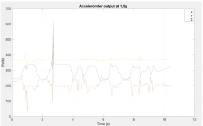
The Breakout has four sensitivity modes: 1.5g, 2g, 4g and 6g. By pressing the pedal with altering forces and with the accelerometer connected to an Arduino, the maximum accel-eration was measured in order to choose an appropriate sensitivity mode. The output of the Breakout in 1,5g mode is shown in figure 2.10 and 2g in figure 2.11 using an Arduino & Processing sketch for making graphs [10]. The spikes in both figures can be ignored be-cause they were formed by the Arduino hitting the ground while moving the pedal. 1,5g mode gave results with enough margin to keep accurately measuring the acceleration. This mode outputs 800mV/g with variance between 740 and 860 mV/g [9], however, ex-act calibration is required during the implementation. The accelerometer also measures gravity, when an axis is perpendicular to the ground it will give a 1g output in the respec-tive axis, this needs to be compensated for an accurate acceleration measurement.
Figure 2.10: Accelerometer output at 1,5g sensitivity
[image:21.595.109.510.400.645.2]2.2.5 Elmo Whistle & power supply
The Elmo Whistle is a motor controller which regulates the current going to the motors. On top of the Elmo Whistle is an Elmo Whistle board as designed by G. te Riet o/g Scholten which provides the required I/O for operation. The Elmo will be used in voltage mode where it takes a voltage between two set-points and translates it into a current to the mo-tor. The position of the pedal is controlled by controlling the voltage. Also connected to the Elmo is a power supply which is used to drive the motors. The power supply in ques-tion is the EA-PS 548-05T [11], capable of delivering between 43V and 58V and 5,2A with a 78% efficiency.
2.2.6 TS7300, YS9700 & TS-XDIO
The existing interface is made with a TS7300 micro controller [12] running 20-sim 4C software [13]. This TS7300 is used as proof of concept, but the board is no longer sup-ported by RaM and therefore needs to be replaced. However, the wiring schematic will be copied because the pedal hardware will stay the same. To connect the accelerometer to the TS7300 and the Elmo whistle (motor controller) [14] to the motor, a TS9700 (AD/DA converter) [15] is placed on top. The encoder is connected to the TS7300 via a TS-XDIO (extended digital IO shield). How the TS7300 and its add-ons will be replaced will be dis-cussed in 2.2.7.
2.2.7 Embedded computer replacement
The pedals need to be connected to an embedded computer in order to be controlled and connected to a network. Two options are compared. The first option is an Arduino, because of prior experience no learning is required, enabling more time allocation for development. Second, a RaMstix is a possibiltiy because it is resourceful and it is devel-oped by RaM and therefore well supported. There are three main requirements for the embedded system to operate correctly:
1. Containing all required I/O 2. Sufficient processing capabilities 3. A connection to ROS (see section 2.4)
Both embedded systems provide sufficient I/O to connect to all sensors and actuators and will not be compared on this characteristic.
2.2.7.1 Arduino
Connection to ROS
ROS and Arduino can easily be connected with the rosserial_arduino [16] package. The package provides a ROS communication protocol that works over Arduino’s universal asynchronous receiver-transmitter (UART) which makes the Arduino a ROS node which can directly publish and subscribe to ROS messages [17]. Also, the IDE from Arduino can be used for developing the node, which makes programming the Arduino relatively easy.
Processing capability
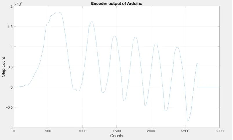
[image:23.595.109.511.396.637.2]A significant limitation of the Arduino is the processor speed in combination with the lack of dedicated encoder inputs. The Arduino uses interrupt pins to add to or subtract from the step count, taking up processing time. A test has been done in order to see whether the Arduino could keep up with counting the steps of the encoder. The pedal was pulled all the way up before starting the counting on the Arduino. During the test the pedal was quickly pushed all the way down and slowly pulled back up again seven times. The results can be seen in figure 2.12. The figure clearly shows that the Arduino counted less steps when the pedal was going down (decreasing the step count) in comparison with going up, meaning it missed steps when the pedal is going too fast. Each position of the pedal should correspond to a unique step count, however missing steps alters this unique step count making the Arduino unusable for position tracking and thus for the implementa-tion.
2.2.7.2 RaMstix
The RaMstix is more a powerful and versatile board than the Arduino, giving it the prefer-ence with respect to future development. The board contains an Overo module with an ARM processor, FPGA and many I/O options. The FPGA and Overo module are able to communicate via a General Purpose Memory Controller. The Overo module runs Linux, and because it is connected to the FPGA, C programs are able to communicate with the I/O components.
Connection to ROS
The RaMstix is able to run Linux which in turn can run ROS and thus multiple ROS nodes. Because Linux on the RaMstix is able to communicate to the I/O, ROS can do the same. Because the board is directly connected to ROS the pedals can be controlled without the need of the PC already present in the cockpit, this is an advantage because any nodes required to run on the master side will not have to share processor resources with nodes not relevant to the pedals.
Processing capability
The RaMstix has a significant advantage over the Arduino in processing capability. It con-tains a processor that is approximately 63 times faster and it has dedicated encoder in-puts. This means that the encoder values are stored in a register and can be requested at any point in time. This is also true for the DAC and ADC values used for the accelerom-eters and Elmos. Therefore the full processor capability is available for the processing of the signals.
2.2.7.3 Conclusion
In the end the RaMstix has been chosen because of the significantly larger capabilities of the system. A comparison table is shown in table 2. Because the Arduino was not able to keep up with one incremental encoder it is not resourceful enough for the use of this project. The RaMstix will be used as embedded computer, limiting time for current development, but enabling future development.
Table 2: Embedded computer comparison
Device Easy of Use Ros Connection Processing Capabilities
Arduino Uno + +
2.3 Pedal controller
In order to control the position and damping of the pedals, a controller is designed using the accelerometer and encoder data as input. Both sensors’ output first needs to be con-verted to SI-units and possibly integrated or differentiated depending on the controller that is used. The pedal controller will also include a variable spring constant for the im-plementation of haptic feedback, this is discussed in section 2.4.2. Note that the controller is in the rotational domain.
Figure 2.13: A schematic overview of the spring and damper connected to the pedal, both the spring and damper are in rotational domain
2.3.1 Harmonic oscillator
The pedals will be controlled to behave like a damped harmonic oscillator. A schematic drawing of the components is shown in figure 2.13. All motion for the pedals is in rota-tional domain. To return the pedal to the origin position, a virtual spring will be used based on the displacement of the pedal with respect to the origin position. This is de-scribed by Hooke’s law as shown in equation 2.3.
Fs= −Kθp (2.3)
WhereFs is the exerted force, K is the spring constant andθp the displacement of the
spring. The constant has a minus sign because the exerted force is in the opposite direc-tion of the displacement of the spring. To prevent the pedal from overshooting its target position, a virtual damper acting as friction is added to the controller based on the veloc-ity of the pedal and a damping coefficient (equation 2.4).
WhereFdis the frictional force,Dthe damping coefficient andωpthe velocity. The
com-bination of the two above equations make the base of the controller and gives the follow-ing equation.
F= −Kθp−Dωp (2.5)
With the controller equation defined, the damping ratio can be tuned to the desired value with the following equation.
ζ= D
2pI K (2.6)
Whereζis the damping ratio,Dthe damping coefficient,I the inertia of the pedal andK the spring constant. The damping ratio will be tuned to be critically damped, this will re-turn the pedal to its origin position as fast as possible while preventing it from oscillating. By rewriting the damping ratio equation as a function ofDwith a damping ratio of 1 as shown in equation 2.7, equation 2.5 can be rewritten as equation 2.8.
D=2pI K (2.7)
F= −Kθp−2ωp
p
I K (2.8)
As described in section 2.1, the haptic feedback implementation will alter the spring con-stant. However, the damping constant in equation 2.8 is now dependent on the spring constant, maintaining a constant damping ratio of 1.
2.3.2 Position
The encoder data will be used to measure the position, compensate gravity in the ac-celerometer and differentiate the position into the velocity. Because the pedal has a lim-ited movement range, there is a finite number of steps divided over the movement range. If the starting position of the pedal is a set position, any number of steps will correspond to a unique pedal position. When the position is requested by the driver, the step count will be converted to a position in radians. The measured resolution of the encoder was 1,85E-3 degrees per step, this converts into 3,23E-5 radians per step. The offset of the pedals is 21,86 degrees which has to be added to the position. The resulting angle will also be used to compensate for the gravity in the accelerometer data, this is discussed in 2.3.3.
2.3.3 Acceleration
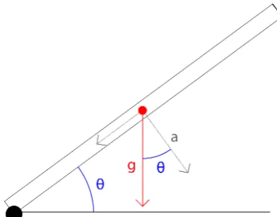
Figure 2.14: The magnitude ofacan be calculated by multiplyinggwith the cosine ofθ
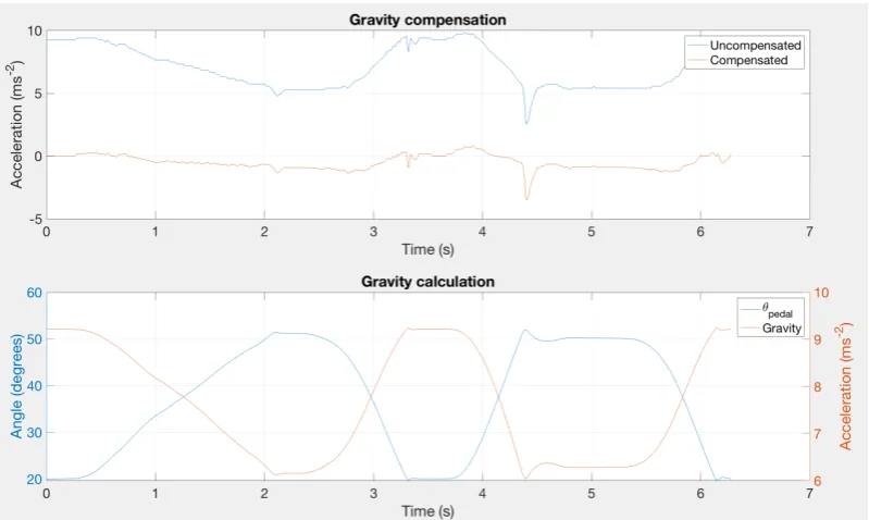
shown in figure 2.14. By taking the cosine ofθand multiplying it byg(9, 81ms−2) and then subtracting this from the measured acceleration, will result in the acceleration without the gravity component. This is tested by measuring both the accelerometer and encoder at the same time when attached to the pedal. The pedal is moved up and down twice. The measured pedal angle is used to calculate the gravity working on the accelerometer. The calculated gravity is subtracted from the measured acceleration, this should result in the acceleration of the pedal without gravity. The output is shown in figure 2.15. (1) shows the acceleration signal before and after the calculated gravity is subtracted (uncompen-sated and compen(uncompen-sated respectively). (2) shows the angle of the pedal and the calculated magnitude of the gravity working on the accelerometer based on the pedal angle. If work-ing correctly, the compensated acceleration in (1) should be 0 when the pedal angle is not changing. This is the case when the pedal is in its lowest position (T≈0s - T≈0,5s), but not in the highest (T≈4,5s - T≈5,5s). Looking at (2) it shows that the compensa-tion is working as expected, a higher angle results in a lower compensated gravity. The error in the compensated acceleration could be causes by inaccurate calibration of both the encoder and accelerometer, this will have to be calibrated during the implementation phase.
2.3.4 Velocity
Figure 2.15: TTB (1) Acceleration signal before and after gravity compensation based on the pedal angle (2) Calculated gravity component based on the angle of the pedal
2.3.4.1 Differentiating position
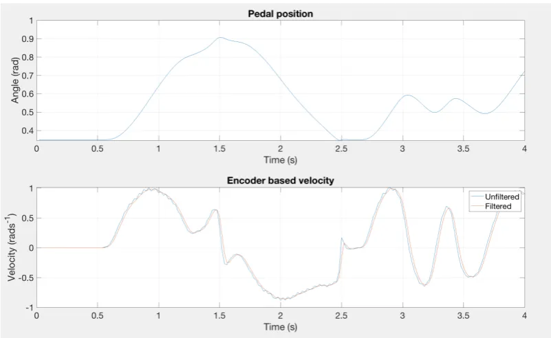
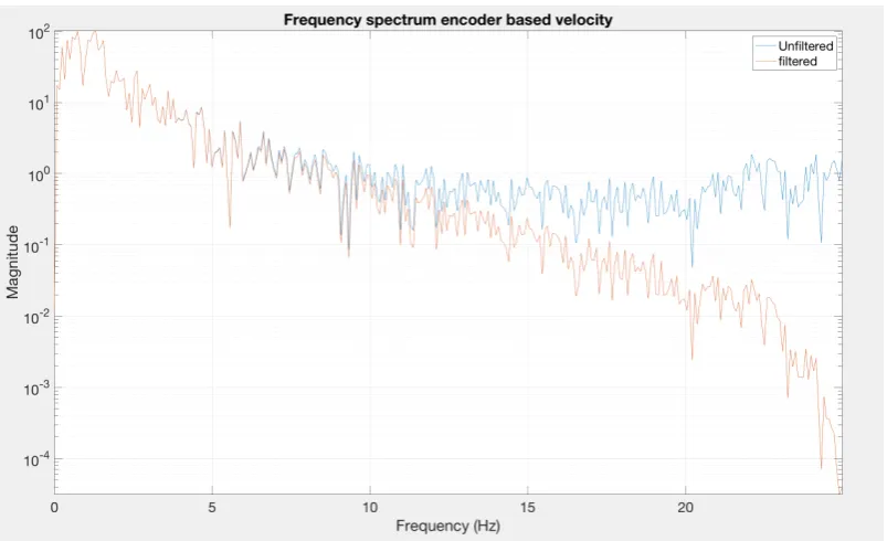
The position signal from the encoder proves to be very suited to differentiate into veloc-ity. Sample data is collected by moving the pedal up and down with the accelerometer attached as shown in figure 2.9 and the encoder connected to the motor, a sample fre-quency of 50hz was used. The pedal angle will be differentiated and then filtered with a low-pass filter to remove the expected high frequency noise. For the low-pass filter a sec-ond order Butterworth filter with a 10Hz cutoff frequency is used. The differentiation and filtering are done using Matlab.
Figure 2.16: TTB (1) Encoder output converted into the angle of the pedal over time (2) The unfiltered and filtered outcome of integrating the position to angular velocity
Figure 2.18: Frequency spectra of the unfiltered and filtered encoder based velocity
2.3.4.2 Integrating acceleration
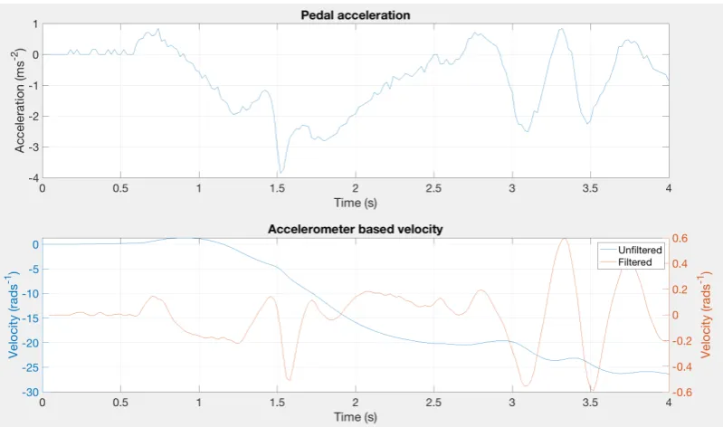
The acceleration signal from the accelerometer is likely to contain an offset and high fre-quencies. This will cause the integrated signal to drift. The implementation of gravity compensation will get rid of a significant part of the offset, but not all. Using a high-pass filter, the remaining offset can be filtered out to create a usable velocity signal. The same sample data as in section 2.3.4.1 is used for testing. After integration a second order 2,5Hz high-pass Butterworth filter is applied to reduce the offset. Both the integration and filter are applied with Matlab.
where the peak in (2) appears later in time than in (1).
Figure 2.20: TTB (1) Frequency response unfiltered accelerometer output (2) Frequency response velocity based on integrated unfiltered accelerometer output
2.3.4.3 Sensor fusion
Both velocity signals from the accelerometer and encoder need to be filtered with a high-pass and low-high-pass filter respectively, which can be used to fuse the signals. Matching the cutoff frequencies of both filters makes it possible to sum the signals. Figure 2.21 shows the diagram of the summation of both signals after a first order filter. By rewriting the transfer function, it is proven that the combined signals equal the velocity. This is shown in equation 2.9 to 2.13.
v(s)=v(s)· 1
s+1+v(s)· s
s+1 (2.9)
v(s)= v(s)
s+1+ sv(s)
s+1 (2.10)
v(s)=v(s)+sv(s)
s+1 (2.11)
v(s)=(s+1)v(s)
s+1 (2.12)
v(s)=v(s) (2.13)
Figure 2.21: Diagram for summing the velocity values after integration/differentiation and filtering
2.3.4.4 Infinite Impulse Response filter
For the digital filtering of both velocity signals an Infinite Impulse Response (IIR) filter will be used. Either a Finite Impulse Response (FIR) or IIR filter can be used, FIR filters have as an advantage that the produces phase lag is linear and therefore predictable compared to IIR filters which have a less predictable phase lag, however, the phase lag is shorter. Because the phase lag is shorter in IIR filters they are more suitable for real-time applica-tions and therefore they are chosen. During the design phase multiple IIR filters will be designed and tested with as goal an accurate velocity estimation using lower frequencies from the encoder and higher frequencies from the accelerometer. Another important as-pect of the filters that needs to be tested is the delay, because when too large, the feedback could be noticeably delayed, reducing the effect of the feedback. The estimated velocity will have a delay of:
Del a y=N
fs
(2.14)
WhereN is the order of the filter andfsthe operating frequency. The filters also introduce
Figure 2.22: Phase shift for a second order high-pass Butterworth filter with a 10Hz (0,4 normalized frequency) cutoff frequency at a 50Hz sample frequency
2.4 Software architecture
[image:35.595.207.412.228.492.2]The software architecture is built up of four different parts: the pedal driver, controller, feedback calculation and interpretation. The communication between the cockpit and the robotic platform is setup using ROS (Robot Operating System). ROS provides a frame-work for writing robot software. The frameframe-work allows for writing code in a modular ap-proach which will be used for the separation of the four parts. A simplified schematic of the interaction between the four nodes (software module) is shown in figure 2.24. This section will elaborate on the function and the in- and output of each node.
Figure 2.24: Overview of the different nodes in ROS to operate the pedals
2.4.1 Pedal driver
Figure 2.25: Graph for the formulay=1x
2.4.2 Pedal controller
The controller node is the node that calculates the force that the pedals will exert onto the user. How this node calculates the force is described in section 2.3.1. This node requires the position and velocity of the pedal for control without haptic feedback. With haptic feedback, the spring constant in the controller is dependent on the distance and location of an obstacle, and the platform’s velocity. Because the increase in spring constant will be calculated in this node, those variables are therefore required as input as well.
To implement the haptic feedback in the controller, the spring constant is made a func-tion instead of a constant. First a base spring constant is required for the operafunc-tion of the pedal without haptic feedback. Then, the increase in spring constant will be deter-mined by the distance to an obstacle. As deterdeter-mined in section 2.1.4, the haptic feedback based on the distance to an obstacle should act like a non-linear spring. More specific, the haptic feedback should become exponentially larger when the platform closes in on an obstacle. The curve should range from maximum spring constant increase at mini-mal detection range to no spring constant increase at maximum detection range. This behaviour is similar to the functiony=1x as shown in figure 2.25, whereybecomes larger whenxdecreases. Therefore the increase in spring constant will be a variation ofy= 1x, tuned to the characteristics of the system. The general equation for this is given in equa-tion 2.15
Kl =
m lo+n+
p (2.15)
WhereKl is the increase in spring constant based on the distance to an obstacle,lo the
Then, to indicate the location of the obstacle, the increase in spring constant is scaled for each pedal based on an algorithm described in section 2.4.3.2. The distribution for each pedal is between 0 and 1, which the increase is multiplied by. Adding to equation 2.15 gives the following equation:
Ki=Kl·U (2.16)
WhereKiis the increase in spring constant based on the distance and location of an
ob-stacle andUthe distribution for the corresponding pedal.
Last, the platform’s velocity is added to the spring increase equation. The faster the plat-form goes, the larger the spring constant should be. However, the feedback should also be noticeable while moving slowly. To accommodate for both requirements, the platform’s velocity is converted to a 0,5 to 1 scale which the spring constant increase is multiplied by. The equation for the conversion is:
V =0, 5vr
vmax +
0, 5 (2.17)
WhereV is the converted velocity,vr the platform’s current velocity andvmax the
plat-forms maximum velocity. Combining equation 2.17 with 2.16 results in the following equation.
Ki=Kl·U·V (2.18)
Adding the final equation for the increase in spring constant to the controller equation (equation 2.8 in section 2.3.1) results in the final controller equation as shown in equation 2.19.
F= −(Kb+Ki)θp−2ωp
p
I(Kb+Ki) (2.19)
WhereFis the output force,Kbthe base spring constant,Kithe spring constant increase,
θpthe pedal position,ωpthe pedal velocity andIthe pedal’s inertia.
2.4.3 Obstacle interpretation
The obstacle interpretation node outputs the distance to, and force distribution based on the relative angle of the obstacle. The node receives two vectors containing the location of the obstacle with respect to the orientation of the robotic platform. The vectors are parallel and perpendicular to the platform, shown in figure 2.26 asXoandYorespectively.
Figure 2.26: Calculation of the obstacle distance based on the input vectors
2.4.3.1 Obstacle distance
To determine the distance to the obstacle, Pythagoras’ theorem can be used. The magni-tude of the combined vector can be calculated as shown in equation 2.20.
lo=
q
Xo2+Yo2 (2.20)
Wherelo is the distance to the obstacle,Xo the vector’s component in parallel direction
andYothe vector’s component in perpendicular direction. The magnitude is then passed
to the controller node as the distance to the obstacle.
2.4.3.2 Obstacle location
For the force distribution, the angle of the vector with respect to the orientation of the robotic platform is used and can be calculated using basic trigonometry.
θo=arctan
Xo
Yo
(2.21)
Whereθois the angle to the obstacle in radians with respect to the direction of the robotic
platform. The angle is then converted to a distribution between the two pedals. Figure 2.27 shows how the conversion of the angle to the obstacle and the distribution between the two pedals will be done. The combined distribution is always 1, resulting in the red diamond shape. The distribution for any vector is based on the point of intersection be-tween the vector’s angleθoand the distribution diamond, point A in figure 2.27. The
Figure 2.27: Calculation of the pedal force distribution based on the obstacle angle
Between 0 and 0,5π:
UL=
0, 5·θo
0, 5π (2.22)
Between 0,5 andπ:
UL=
0, 5·(θo)
0, 5π (2.23)
Betweenπand 1,5π:
UL=0, 5+
0, 5·(0, 5π− |θo|)
0, 5π (2.24)
Between 1,5πand 2π:
UL=1−
0, 5·(0, 5π−θo)
0, 5π (2.25)
Because the combined distribution is always 1, the distribution for the right pedal is:
UR=1−UL (2.26)
2.4.4 Pedal interpretation
and backwards at maximum velocity and clockwise and counterclockwise rotation on the spot. In order to achieve all four motions with the two pedals, the pedal position is inter-preted as shown in figure 2.28. Each pedal controls its corresponding side of the robotic platform. The pedal controller is supposed to have its origin position in the centre of the pedal range, allowing for motion in two directions. Pushing the pedal downwards results in a forward motion on the robotic platform, and pulling the pedal up results in a back-wards motion. Using two pedals, all four extremes of motion can be achieved.
Figure 2.28: Pedal range and corresponding direction
For the conversion of the pedal positions to a twist, the pedal range is first converted to a displacement of -50% to 50% with 0 being the origin position. Using this range, all motions are based on the ratio between the two pedals. Moving forwards at maximum velocity, both pedals are at 50% summing up to 100% with a 0% difference. For a clockwise rotation on the spot the left pedal is at 50% and the right at -50%, making the sum 0% and the difference 100%. Table 3 gives the pedal values for all four extreme motions and the corresponding sum and difference. The sum and difference are then used for the twist’s linear and rotational speed. Using the predefined maximum velocity for the wheels multiplied by the sum and difference for the linear and rotational velocity respectively, to construct a twist.
Table 3: Extreme motions, corresponding pedal positions and resulting twist
Motion extremes Pedal values
<%Left, %Right> Sum Difference
Twist
<Linear, Rotational>
3 Design & implementation
[image:41.595.168.451.235.612.2]In this design and implementation section the design based on the plan in the analysis will be discussed. First, the RaMstix setup will be discussed in section 3.1. All connection diagrams, hardware components and specifications are documented in this section. Sec-ond, the software architecture for the system is written and divided in parts called nodes in section 3.2. Each node is described in terms of input/output and all the functions it fulfils. And finally, in section 3.3 the mechanical alterations are discussed. The final im-plementation is shown in figure 3.1.
3.1 Electrical
[image:42.595.140.427.211.521.2]Because the embedded computer (TS-7300) is replaced by a RaMstix, all connections will need to be redone. In this section all the new hardware connections will be described and illustrated. Illustrations will be based on figure 3.2 and 3.3. Figure 3.3 is a connection board for SV10, X5 and X6 of the RaMstix. K3 and K4 on the connection board can be used for extended signal processing, this is not used and are therefore directly connected.
Figure 3.3: Schematic pin overview of the connection board to the RaMstix
3.1.1 Encoder
The encoders will be connected to the RaMstix’s encoder inputs via the connection board. SV10 in figure 3.2 has connections for up to four encoder inputs, one 5V output and ground connections. The first two encoder inputs have been wired to K1 on the con-nection board, including the 5V output and ground. The two used encoders are wired to encoder input 1 & 2 as shown in figure 3.4. The index pin does not have to be connected since the encoder register will be reset every reboot as explained in section 2.2.3, but will be connected for possible future implementation.
3.1.2 Accelerometer
Figure 3.4: Schematic wiring of the encoders to the connection board
[image:44.595.165.409.403.648.2]Figure 3.6: Schematic wiring of the motors connected via an Elmo Whistle to the RaMstix, the Elmo is connected to a power supply to drive the motors
3.1.3 Motor, Elmo Whistle and power supply
The motors are controlled by an Elmo Whistle each, which regulate the current going to the motors. A schematic drawing of the wiring is shown in figure 3.6. The Elmos are directly connected to the RaMstix. The power used to drive the motors is supplied by two power supplies directly connected to the Elmos. The set-point for the output current of the Elmo is regulated with an analog voltage supplied by the RaMstix. The RaMstix is able to output a voltage of±2,5V from the DAC. The motors have a maximum continuous current of 4,58A, which in combination with the DAC voltage translates into a 1,832A/V control ratio, both positive and negative.
3.2 Software
Figure 3.7: Schematic overview of the software architecture including the signal flows
3.2.1 ROS usage
[image:46.595.102.471.95.306.2]For the communication between different nodes, ROS uses topics on which messages are send. Messages can be standard or custom made and can be communicated in different ways. For this software architecture two communication protocols will be used: asyn-chronous and synasyn-chronous. A synasyn-chronous communication consists of one client and one server. The client sends a request to the server and waits for a reply. The server will only send a message whenever it receives a request. A visual representation is shown in figure 3.8. In an asynchronous communication there is a topic to which can be published or subscribed without the need of a request. Multiple publishers can publish to the topic and multiple subscribers can subscribe to the topic at the same time. A visual represen-tation with one publisher and multiple subscribers is shown in figure 3.9.
Figure 3.9: Schematic overview of a asynchornous communication with one publisher and three subscribers
3.2.2 Pedal driver
The pedal driver node is a node that requests the sensor values from the RaMstix and converts them into SI units which can be used by the other ROS nodes. The node also estimates the velocity of the pedal based on the position and acceleration. The node will have three main functions which are described in this section: requesting sensor values, converting sensor values and estimating velocity. A schematic overview of the in- and output of the pedal driver node is shown in figure 3.10.
3.2.2.1 Requesting sensor values
For the communication between the RaMstix and the pedal driver node, the ZeroMQ [19] library has been used. ZeroMQ provides the same synchronous communication as with ROS. First, the received output force from the controller node is mapped to the DAC’s output range. Then, the pedal driver node sends a request to the RaMstix, containing the output voltage values of the controller. The RaMstix then sets the DACs to the re-ceived voltages and retrieves the sensor values from the registers. The encoder counts and accelerometer voltages are send back as the reply message to the pedal driver node. A synchronous communication is used in order to set the frequency at which the RaMstix runs from the pedal driver node.
3.2.2.2 Standardising sensor values
In the pedal driver node the received sensor values from the RaMstix are converted into SI units. First the encoder steps are converted to radians using the 3,23E-5r ad/st epand the 21,86° (3,82E-1r ad) offset, determined in section 2.3.2, as shown in equation 3.1.
θp=3, 82E−1+xenc·3, 23E−5 (3.1)
Whereθpis the pedal angle in radians andxencthe pedal position in steps.
Next, the accelerometer voltage is converted tor ad s−2. The accelerometer has an offset voltage which is subtracted from the measured voltage. Then the voltage is divided by the sensitivity of the accelerometer and multiplied by the gravitational force (9,81ms−2), resulting in the acceleration inms−2.
ames=
(Vi n−Vo f f)·g
Sacc
(3.2)
Where ames is the measured acceleration inms−2,Vi n the measured voltage,Vo f f the
offset voltage of the accelerometer,gthe gravitational force andSaccthe accelerometer’s
sensitivity.
Then the signal is compensated for gravity as discussed in section 2.3.3 of the analysis, resulting in equation 3.3.
acomp=
(Vi n−Vo f f)·g
Sacc −
cos(θp)·g (3.3)
Whereacompis the compensated acceleration inms−2andθpthe position of the pedal in
radians.
For the conversion fromms2tor ad s−2, equation 3.4 is used.
v=rω (3.4)
Combining equation 3.3 and 3.4 result in equation 3.5 for the calculation of the rotational acceleration of the pedal.
ap=
Vi n−Vo f f
Sacc ·g−cos(θp)·g
racc
(3.5)
Whereapis the pedal acceleration inr ad s−2andracc is the radius of the motion of the
accelerometer inm.
3.2.2.3 Calculating velocity
Using the pedal position and acceleration to estimate velocity, they need to be differenti-ated and integrdifferenti-ated respectively. For differentiating the position the difference quotient is used as shown in formula 3.6.
ω(t)≈θp(tk)−θp(tk−1)
∆tk
(3.6)
Whereω(t) is the angular velocity,θp(t) the pedal’s position,tthe time andkthe current
measurement.
For the integration of the acceleration the trapezoidal rule is used as shown in formula 3.7.
ω(t)≈
N
X
k=1
a(tk)+a(tk−1)
2 ∆tk (3.7)
Whereω(t) is the angular velocity, a(t) the pedal’s angular acceleration,tthe time andk the current measurement.
After both velocities are acquired, they are filtered to prevent noise and allow sensor fusion as described in section 2.3.4.3 of the analysis. Two cut-off frequency matched second-order Butterworth filters are used, one being a low-pass and the other a high-pass filter. Both are IIR filters using the general transfer function as shown in equation 3.8, with coefficients generated by Matlab.
ωf[tk]=
1 b0
à P X
i=0
ciωu[tk−i]− Q
X
j=1
bjωf[tk−j]
!
(3.8)
Where:
• ωf is the filtered angular velocity
• ωuis the unfiltered angular velocity
• biare the feedback filter coefficients
• ciare the feedforward filter coefficients
Both filters have a 10Hz cutoff frequency at a 200Hz sample frequency. The frequency response and phase shift are shown in figure 3.11 and 3.12 for the low-pass and high-pass filter respectively. After both velocity signals are filtered, they are summed and send to the controller node.
Figure 3.11: Plot of the frequency response and phase lag of a second order low-pass But-terworth filter with a cutoff frequency of 10Hz and a sampling rate of 200Hz
Figure 3.12: Plot of the frequency response and phase lag of a second order high-pass Butterworth filter with a cutoff frequency of 10Hz and a sampling rate of 200Hz
3.2.3 Controller
Figure 3.13: Schematic overview of the in- and output of the spring-damper node
First, a base spring-damper controller based on section 2.3.1 of the analysis is imple-mented. The base controller operates without haptic feedback (Ki = 0) and has a
min-imum spring constantKb to return the pedal to its origin position. First, an offset force
is added to the output force to counter the gravity as result of the weight of the pedal. Adding a force offset to equation 2.19 of the analysis withKi=0 results in equation 3.9.
Fout= −Kbθp−2ω
p
I Kb+Fo f f (3.9)
WhereFoutis the output force of the controller,Fo f f the offset force,Kbis the base spring
constant,ωthe rotational velocity andI the pedal’s inertia.
Without haptic feedback, the pedal should exert a large enough force to not feel loose, but small enough to not be perceived as feedback. To achieve a tight feeling, the square root of the displacement is taken because of the square root’s shape as shown in figure 3.14. A small displacement results in a relatively large output force, preventing accidental movement when a foot is rested on the pedal. Altering equation 3.9 gives equation 3.10, forming the base spring-damper algorithm for the controller.
Fout= −Kb
q
θp−2ωp
p
I Kb+Fo f f (3.10)
WhenKi 6=0, the spring constant is a function of the distance to an obstacle, force
dis-tribution and velocity of the robot. The distance to an obstacle and the robot velocity are converted toKi andV, using equation 2.15 and 2.17 of the analysis respectively as
shown in figure 3.13. Then,Kl,U andV are multiplied resulting inKi. Ki andKb are
then summed, resulting inK.IncludingKiin equation 3.10 results in equation 3.11 as the
transfer function of the controller node.
Fout= −(Kb+Ki)
q
θp−2ω
p
Figure 3.14: Graph for the formulay=px
3.2.4 Obstacle interpretation
The obstacle interpretation node is subscribed to the obstacle location message and pub-lishes a message containing the force distribution for the pedals and the distance to the obstacle. The signal flows of the node are shown in figure 3.15.
Figure 3.15: Schematic overview of the signal flows of the obstacle interpretation node
The obstacle location message contains two vectors, a parallelXoand a perpendicularYo
with respect to the robot direction, as described in section 2.4.3. Using equation 3.12, the distance to the obstaclelois calculated.
lo=
q
X2
o+Yo2 (3.12)
θo=arctan
Xo
Yo
(3.13)
Whereθois the relative angle to the obstacle in radians. Then, equation 3.14 to 3.17 are
used to determine the force distribution on a 0 to 1 scale for the left pedal.
θobetween 0 and 0,5π:
UL=
0, 5·θo
0, 5π (3.14)
θobetween 0,5 andπ:
UL=
0, 5·(θo)
0, 5π (3.15)
θobetweenπand 1,5π:
UL=0, 5+
0, 5·(0, 5π− |θo|)
0, 5π (3.16)
θobetween 1,5πand 2π:
UL=1−
0, 5·(0, 5π−θo)
0, 5π (3.17)
WhereUL is the distribution for the left pedal. The equation for the distribution for the
right pedal is shown in equation 3.18.
UR=1−UL (3.18)
3.2.5 Pedal interpretation
The pedal interpretation node contains the algorithm for converting the pedal position into a twist as described in section 2.4.4 of the analysis. Because the robotic platform is assumed to move with two degrees of freedom, the parallel linear velocity and the angular velocity for yaw are used of the twist. This node subscribes to the message from the pedal driver node containing the pedal positions, and publishes the twist to the control node of the robot. A schematic overview of the signal flows of the node is shown in figure 3.16. As described in section 2.4.4 of the analysis, the pedal positions are first converted to the displacement in percentage with respect to the origin. The equation for the conversion is shown in equation 3.19.
P=100·(θp−θmi n)
θmax−θmi n −
50 (3.19)
WhereP is the displacement percentage between±50% for one pedal, θp the received
pedal position andθmaxandθmi nthe pedal position’s extremes in radians.
Then, using either the sum or the difference between both displacement percentages, the linear and angular velocities are calculated respectively. The formula for the linear movement is shown in formula 3.20.
vl=
vmax·(PL+PR)
Figure 3.16: Schematic overview of the in- and output of the pedal interpretation node
Wherevlis the the linear velocity,vmaxthe maximum velocity of the robotic platform and
PL&PRthe displacement percentages of the pedals. The formula for the angular velocity
is shown in formula 3.21.
vr=
vmax·(PL−PR)
100 (3.21)
Wherevr is the angular velocity.
3.3 Mechanical
4 Testing & results
After the design & implementation phase, all the different parts of the system are tested to be able to evaluate its performance. All tests that involve the pedals will be performed using the right pedal. The reason being that the left pedal does not contain an accelerom-eter. Also all tests are conducted with the pedal controller node, and thus the RaMstix, running at a 200Hz frequency. The test phase contains two parts: the first one is about testing the sensor signal processing, PD controller and controlling the robot, and the sec-ond part is about testing the feedback implementation.
4.1 Pedal tests
In the first part of the testing phase the sensor data acquisition, processing and imple-mentation is tested.
4.1.1 Pedal angle
First, the accuracy of the pedal angle measurement is determined. The pedal angle is used for determining the pedal’s displacement, velocity and acceleration compensation, and therefore the fundament of the whole system. By determining the precision of the pedal angle measurement, other components can be validated as well.
The measured angle of the pedal is compared to the measured angle in section 2.2.1 of the analysis chapter. This test will provide the precision of ther ad/st epconversion. To determine the precision of the measurement, the pedal is placed in its minimum and maximum angle. The output values are compared against the physically measured angle. The accuracy is presented in percentage based on formula 4.1.
Q= 100·θexp
θexp+(|θexp−θmes|)
(4.1)
Where Q is the precision in percentage,θpis the pedal position in radians,θexp the
ex-pected angle andθmesthe measured angle. It is expected that the output angle will at least
have a precision 98,74% of the expected angle. This is based on the encoder calibration and the encountered error in the step count. The encoder is calibrated at 3,2309E-5 radi-ans per step and during testing a maximum error of±150 steps was encountered.
Table 4: Results pedal angle test Position Expected (radians) Measured (radians) Delta Accuracy (%) Min 3,80830843E-1 3,81528974E-1 6,98131E-4 99,82
Max 9,07920277E-1 9,08618409E-1 7,98132E-4 99,91
4.1.2 Acceleration and gravity compensation
The measured acceleration is used for estimating the velocity signal’s higher frequencies, to determine the usability of the measured signal the gravity compensation and noise in the signal are examined. The acceleration before and after the compensation are com-pared to determine the effectiveness of the compensation. The compensated signal will also shown errors in the calibration of the accelerometer. Last, the compensated acceler-ation signal is examined in frequency domain to evaluate the noise.
For the testing of both the uncompensated and compensated acceleration signal, test data is acquired by saving the output of the pedal angle, uncompensated acceleration and compensated acceleration over multiple pedal angles. The pedal is placed in an an-gle and then held in position to remove any movement acceleration. Both acceleration signals are plotted against the pedal angle. To examine the noise, the compensated accel-eration signal is plotted in frequency domain.
The hypothesis is, that without pedal motion the uncompensated signal outputs the mag-nitude of gravity working on the accelerometer. Increasing the pedal angle is expected to result in a decrease in output. For the compensated acceleration, it is expected that the acceleration is 0 for every pedal angle. The angle measurement of the encoder is eval-uated sufficiently good, therefore the gravity compensation is expected to be reliable as well. During motion, both accelerations are expected to behave similar, excluding the off-set in the uncompensated acceleration. Going from one pedal angle to the next should show a spike in both acceleration signals. If the accelerometer is not correctly calibrated, the compensated acceleration signal will either have an offset or not be horizontal.
During motion, in figure 4.2 shown in the areas between the vertical lines, the deviation for both signals is approximately equal to the deviation without motion. During the first motion between 0,37 and 0,55r ad, both signals have a deviation larger than the constant deviation. However, for the other three moments of motion, the deviation does not exceed the deviation without motion. This means that, if the acceleration is not large enough, it is drowned out by the deviation.
The frequency spectrum of the compensated acceleration signal is shown in figure 4.3. It shows a large 0Hz magnitude, confirming that the signal still has an offset. It is also visi-ble that the signal contains lower frequencies with a relatively high magnitude, indicating that the acceleration signal does contain the motion of the pedal. It does not show an outstanding peak in the higher frequencies, indicating that the noise is present in a broad frequency range.
Based on the observation that the accelerometer output is consistent, but including noise, the output voltage of the RaMstix was tested by connecting the DAC directly to the ADC and subtracting the mean offset of the signal. The output is shown in figure 4.4 and its corresponding frequency spectrum in figure 4.5. The frequency spectrum shows that the noise in the output voltage is over the full range of frequencies, but with a very small mag-nitude and therefore unlikely to cause the noise in the acceleration signal. Due to time constraints, the cause of the noise has not been found.
Figure 4.2: The uncompensated and compensated acceleration signal against the pedal angle
[image:58.595.87.486.413.660.2]Figure 4.4: Output of the RaMstix DAC directly to the ADC
[image:59.595.109.511.391.634.2]4.1.3 Sensor Fusion
The goal of this test is to assess the added value of using sensor fusion for the velocity estimation of the pedal. This is determined by the results of the differentiation of the po-sition, integration of the acceleration and low- and high-pass filters. The output values of time, pedal angle, differentiation, integration, LPF, HPF and the combined velocity are recorded during random pedal movement. Then the output signals are compared both in time and frequency domain. The same set of values will be used for this entirety of this section. The output of the pedal angle over time is shown in figure 4.6, and in fre-quency domain in 4.7. For the frefre-quency spectrum notice that the range of frequencies displayed is only 0 to 10Hz, also the 0Hz offset is vertically cutoff die to the relatively large magnitude.
Figure 4.7: Output of the pedal position in frequency domain
4.1.3.1 Differentiation & low-pass filter
Differentiating the pedal position into velocity amplifies the high frequency noise in the signal, therefore the goal of this test is to see whether the differentiation produces a usable signal and if the low-pass filter improves it. Based on the findings in section 2.3.4.1 of the analysis, it is expected that in the peaks of the velocity signal high frequency noise will be present. Which in turn will be filtered out by applying the low-pass filter. The filtered velocity is expected to have a 10ms delay based on the second order filter and the 200Hz sampling frequency.