Parametric dynamic survival models

University of Warwick institutional repository:http://go.warwick.ac.uk/wrap A Thesis Submitted for the Degree of PhD at the University of Warwick

http://go.warwick.ac.uk/wrap/73391

This thesis is made available online and is protected by original copyright. Please scroll down to view the document itself.

Parametric Dynamic Survival

Models

by

Karla Hemming

A thesis submitted for the degree of Doctor of Philosophy

Department of Statistics

University of Warwick

Coventry

CV47AL

Contents

1 Introduction

2 Survival Analysis

2.1 Censoring and Truncation . . . . . 2.2 The Survival and Hazard Functions 2.3 The Likelihood . . .

2.4 The Bayesian Approach

2.5 Survival Models . . . . . 2.6 Non-proportional Hazards 2.7 Methods for Model Fitting . 2.8 Interval Censoring . . . .

2.9 Double Interval Censoring 2.10 Frailty . .

2.11 Summary

3 Dynamic Survival Models

3.1 The Dynamic Bayesian Model for Survival Data 3.2 Parametric Dynamic Survival Models . . . .

3.2.1 Conditional Survival Functions (1) 3.2.2 The Temporal Factorisation . . . . 3.2.3 Conditional Survival Functions (2) 3.2.4 Conditional Survival Functions (2B) 3.2.5 The Individual Factorisation.

3.2.6 MCMC Implementation

3.2.7 Convergence Diagnostics 3.3 Gastric Cancer Data Analysis

3.4 Summary . . . . . . .. 95

4 Flexible Dynamic Survival Models

4.1 Conditional Survival Functions (3) 4.2 Interval Censoring . . . . .

4.2.1 The Likelihood .. . 4.3 Double Interval Censoring . 4.3.1 The Initiating Event 4.3.2 The Terminating Event.

4.4 F r a i l t y . . .

4.4.1 The Normal Dynamic Frailty Model (NDFM) .. 4.4.2 Interval Censoring and Frailty ..

4.4.3 Individual Frailties . 4.5 Summary .

5 Model Fitting

5.1 Gibbs Sampling . . . . 5.1.1 The Full Conditionals

5.1.2 Metropolis-Hastings . 5.2 Imputation Methods . . . .

5.2.1 Interval Censoring .

5.2.2 Double Interval Censoring . . . . 5.3 Simulation Study

5.4 Summary . . . .

6 Data applications

6.1 Breast Cancer Data .

6.1.1 Analysis using the NDSM . . . .

ii

.

..

97 99

.100

· 101 .102

.105 .106

· .110 · . 111

· .117 · .119 · .127

128

· 128 · 129

· . 135 · .. 136 · .. 138 · .. 140

· .. 142 · .. 150

151

6.2 Kidney Infection Data . . . . 6.3 AIDS Data . . . .

6.3.1 Analysis of Times of Infection

6.3.2 Analysis of Incubation Time .

7 Conclusions and Discussion

7.1 Summary . . . .

A Data Frames and Preliminary Analysis

A.l Gastric Cancer Data . .

A.2 Breast Cancer Data . A.3 Kidney Data. .

A.4 AIDS Data

..

B Simulation Code

iii

· 162 · 169

· 171 · 176

181

· 189

191

· 191

· 198 .205 .213

.225

List of Figures

1 Gastric Cancer: Survival Function . 89

2 Gastric Cancer: Log-baseline Hazard 90

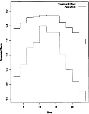
3 Gastric Cancer: Treatment Effect . . 91

4 Gastric Cancer: Proportional Hazards (NDSM) 92

5 Gastric Cancer: Survival using Individual Frailties . · 123

6 Gastric Cancer: Survival using Individual Frailties (2) . .124

7 Gastric Cancer (with Frailties): Esimated Log-Baseline Hazard 125 8 Gastric Cancer (with Frailties): Estimated Treatment Effect · 126

9 Right Censored Simulated Data: Group1 . . .144

10 Right Censored Simulated Data: Group2 . . .145

11 Interval Censored Simulated Data: Group1 . .146

12 Interval Censored Simulated Data: Group2 . .147

13 Double Interval Censored Simulated Data .148

14 Breast Cancer: Survival Function _{· 158}

15 Breast Cancer: Treatment Effect · 159

16 Breast Cancer: Log-baseline Hazard . · 160

17 Breast Cancer: Proportional Hazards (NDSM) . · 161

18 Kidney Data: Survival Function . . · 166

19 Kidney Data: Log-baseline Hazard .167

20 Kidney Data: Covariate Effect . . . . _{· 168}

21 AIDS Data Initiating Event: Covariate Effects · 172 22 AIDS Data Initiating Event: Survival Function · 173 23 AIDS Data Initiating Event: Log-baseline Hazard .174

24 AIDS Data Terminating Event: Survival Function . .178 25 AIDS Data Terminating Event: Covariate Effects

.

26 AIDS Data Terminating Event: Log-baseline Hazard . . . 180

27 Gastric Cancer: Kaplan-Meier . . . 192

28 Gastric Cancer: Cox . . . 193

29 Gastric Cancer: Test of Proportionality. . 194

30 Gastric Cancer: Gibbs Sampling Output . 197

31 Breast Cancer: Thrnbull's Estimate . . 199

32 Breast Cancer: Cox . . . 200

33 Breast Cancer: Test of Proportionality . . . . 201

34 Breast Cancer: Gibbs Sampling Output. . . . 204

35 Kidney Data: Kaplan-Meier . . . 206

36 Kidney Data: Cox . . . . 207

37 Kidney Data: Test of Proportionality . . . 208

38 Kidney Data: Gibbs Sampling Output . . . . 212

39 AIDS (Initiating): Lightly Treated Thrnbull's Estimate. . 215

40 AIDS (Initiating): Test of Proportionality (1) . . . . 216

41

42

43

44

45

46

AIDS (Initiating): Test of Proportionality (2) . . . . 217

AIDS (Terminating): Lightly Treated Thrnbull's Estimate . 218

AIDS (Terminating): Heavily Treated Thrnbull's Estimate .. 219

AIDS (Terminating): Test of Proportionality (1) . . . . 220

AIDS (Terminating): Test of Proportionality (2) . . . 221

List of Tables

Gastric Cancer: Time Axis Comparision

Gastric Cancer: Number of Iterations Comparision Gastric Cancer: Individual Frailties.

Gastric Cancer Data . . . .

Gastric Cancer: Numerical Output Gastric Cancer: Summary Output . Breast Cancer Data. . . .

Breast Cancer: Numerical Output .. Breast Cancer: Summary Output

Kidney Data. . . . Kidney Data: Numerical Output Kidney Data: Estimated Frailties

Kidney Data: Estimated Frailties (continued) AIDS Data: Lightly Treated Group . . . . AIDS Data: Heavily Treated Group . . . .

AIDS Data Initiating Event: Numerical Output

AIDS Data Terminating Event: Numerical Output AIDS Data Terminating Event: Imputation Output Simulated Data: Summary Output . . . .

93

94

· 122

· 191

· 195

· 196

Acknowledgements

I would like to thank my supervisor Ewart Shaw for all of his help

and guidance over the past 3 years, and the EPSRC for supporting

me financially. I wish to thank also my colleagues for their valuable

help. Finally thanks to Henry, my family and Pete.

Declaration

Summary

A non-proportional hazards model is developed. The model can

accommodate right censored, interval censored and double interval

censored data sets. There is also an extension of the model to include multiplicative gamma frailties.

The basic model is an extension of the dynamic Bayesian survival

model developed by Gamerman (1987), but with some alterations and

using a different method of model fitting. The model developed here,

the Normal Dynamic Survival Model, models both the log-baseline

hazard and covariate effects by a piecewise constant and correlated

process, based on some division of the time axis. Neighbouring

piece-wise constant parameters are related by a simple evolution equation:

normal with mean zero and unknown variance to be estimated.

The method of estimation is to use Markov chain Monte Carlo simu-lations: Gibbs sampling with a Metropolis-Hastings step. For double

interval censored data an iterative data augmentation procedure is

considered: exploiting the comparative ease at which interval

cen-sored observations may be modelled.

The model is applied within a range of well known, and illustrative

data sets, with convincing results. In addition the impact of censoring

General Notation

D Data including observations and priors.

i

=

rvr

i

=

K Number of observed covariates.

k = 1, ... , K Subscript for covariates.

ns

rvr

T

Number of individuals in the initiating study population.

Number of individuals in the study population.

Survival times.

T = X - S Survival time based on observing X and S.

t

S

s

X

Survival or censoring time for individual i.

Survival time for the initiating event.

Observed value of S.

Calendar time of terminating event.

Time Axis Notation

(3j

Dj

Dynamic parameter for model.

Information observed up to time tj.

Gs = {so, sI, ... , SNs} Time axis division for initiating model.

GT =

{to,

Ij = (Sj-17 Sj] Interval on the initiating time axis.

Ij = (tj-t, tj] Interval on the time axis.

j

=

j

=

Ns

NT

Sj

tj

Subscript for interval points on the initiating time axis.

Subscript for interval points on the time axis.

Number of intervals on initiating time axis.

N umber of intervals on time axis.

Point on the initiating time axis.

1

Introduction

Cox's proportional hazards model permits the impact of covariates on

sur-vival to be estimated, and using the partial or marginal likelihood approaches

as in Cox (1972) and Kalbefieisch and Prentice (1980), estimates for the

model parameters have been shown to have the same asymptotic properties

as the maximum likelihood estimates (Tsiatis, 1981). Over the last three

decades the model has been heavily used: it has formed a large part of the

basis of statistical research in survival analysis, and has become probably the

most commonly used multivariate survival model in medical applications. Its

major drawback is the constraint of proportional hazards: an assumption

which is not always appropriate. The consequences of using such a model

when the assumption is not appropriate can be high, and for instance may

result in the conclusion of a single superior treatment, when infact this may

not be the case (Carter et al., 1983). Aware of the constraints of the

propor-tional hazards model, Gore et al. (1984) fitted several proportional hazards

models in consecutive intervals (being careful to ensure an adequate amount

of data within each of the intervals), thus avoiding an overall proportional

hazards assumption. The method is not ideal; will only work with large data

sets; and is very sensitive to the number and location of the intervals. Carter

et al. (1983) included treatment multiplied by time as a time dependent

can be extended to model other polynomial changes). Gamerman (1987)

used a piecewise constant baseline hazard and covariate effect, relating

inter-val estimates by a simple semi-parametric relationship. Parameter estimates

are sequentially updated as additional data are received, using conjugate and

linear Bayes approximations, finally sequencing backwards through the

in-tervals to obtain smoothed retrospective estimates. The piecewise constant

correlated process (often abbreviated to piecewise correlated process), is an

attractive way to model both the baseline hazard and covariate effects. Gray

(1992), amongst others, used cubic splines to model both the baseline hazard

and covariate effects over time. Apart from the quoted alternatives above,

there exist few other survival models which are not based on the proportional

hazards assumption.

For interval censoring, double interval censoring and frailty models

(non-independent observations), similar constraints exist in that the majority, if

not all, of the multivariate models are again based on Cox's proportional

hazards model. Piecewise correlated functions have been used to model the

baseline hazard for more complicated censoring types (Ghosh and Sinha,

1995), but the method has never been extended to modelling dynamic

co-variate effects. One of the main reasons for this has been the difficulty in

In this thesis a Markov chain will be constructed with a posterior

distri-bution which models the data by piecewise correlated functions for both the

baseline and covariate effects: thus avoiding the constraints of proportional

hazards, and at the same time overcoming the usual difficulty of estimating

model parameters. The model will be applied to standard right censored

data, and also to additional types of censoring such as interval censoring,

double interval censoring, and frailties. For right censored data the method

will be an alternative to that proposed by Gamerman (1987). For more

com-plicated data types, a non-proportional hazards model will thus have been

developed.

In Chapter 2, many of the standard survival analysis methods are introduced

(including both frequentist and Bayesian methods). A discussion is given as

to why proportional hazards may sometimes be an unreasonable

assump-tion to make, and some alternative methods are suggested. Recent advances

in model fitting techniques are explained, and the method of Markov chain

Monte Carlo (MCMC), including Gibbs sampling and Metropolis-Hastings,

are described. Additional types of censoring (interval censoring, double

inter-val censoring, and also non-independent observations), the problems which

In Chapter 3, Gamerman's model (Gamerman, 1987) is introduced, and the

method for estimating model parameters outlined. It is firstly noted how the

paramater which determines the amount of evolution from interval to interval

(the evolution variance) must be specified prior to model fitting. Secondly it

is observed that the method used by Gamerman to fit the model could not

be extended to accommodate interval, double interval censoring, or frailty

models. For these reasons, a parametric version of Gamerman's model is

introduced, called the Normal Dynamic Survival Model (NDSM). The model

has the same basic structure as in Gamerman (1987) but assumes that the

evolution of the parameters follows a normal distribution (it also models

the evolution variance as a hyper-parameter). It is a parametric model, but

only weakly so, and the model remains sufficiently flexible to accommodate a

wide range of both proportional and non-proportional hazard functions. The

model does however have one disadvantage, and that is no smooth estimates

of covariate effects and baseline hazard exist, although survival estimates are

smooth. To estimate model parameters, Gibbs sampling with a

Metropolis-Hastings step is used. It is noted how Gibbs sampling could not be used in

the semi-parametric model developed in Gamerman (1987), as without

mod-elling the evolution by some parametric distribution, the full conditionals

reparametrisation is introduced, and the likelihoods are based on a temporal

factorisation. The method is illustrated on a set of gastric cancer survival

times (Gamerman, 1987). The development of the NDSM, and data

appli-cations using this model are new developments.

In Chapter 4, likelihoods are developed under the same Normal Dynamic

Survival Model, for extended censoring types (including interval censoring,

double interval censoring, and frailties). For interval censoring, the likelihood

is fairly straightforward, and uses only a slight extension of the conditional

survival functions (developed in Chapter 3 and which were used within the

construction of the likelihood for the right censored model). For double

inter-val censoring, it is observed that the exact likelihood can not be derived, and

so an approximation is given in its place. For both interval censoring and

dou-ble interval censoring, it is not possidou-ble to create a temporal factorisation of

the likelihood and so a factorisation over each observation (individual

factori-sation) is derived as an alternative. For the right censored frailty model, the

likelihood is first given as a temporal factorisation, and secondly as a

factori-sation over the groups: so that the most efficient factorifactori-sations may be used

to compute different full conditionals. Likelihoods are similarly developed for

the interval censored frailty models (it is also described how the likelihood

a small discussion is given on the concept and use of individual frailties. All of

the work within Chapter 4 is new work, although some similarities may exist

between likelihoods of others, and where this is the case it will be made clear.

In Chapter 5, it is shown how Gibbs sampling can be used to estimate the

model parameters using the likelihoods developed in Chapter 4. For double

interval censoring it is explained how either the approximate likelihood could

be used in a full likelihood analysis using Gibbs sampling; or as an

alterna-tive, a method using imputation is outlined, where the data is augmented

to interval or right censored data as appropriate. Applying MCMC

tech-niques to survival data is by now a common feature. The techtech-niques within

this Chapter are not original, but applying them to the NDSM is. As with

the right censored model, a reparmeterisation is used: finding an effective

reparmeterisation is quite a common procedure, Gamerman (1998) also

sug-gested it within the context of a dynamic generalised linear model, although

work here was completely independent. Aslanidou

et

con-structed full conditionals for the frailty parameters in a similar model, and

those full conditionals do bare some similarity to those constructed here,

al-though their model is a proportional hazards model. To examine the impact

that the degree of censoring has on the model, data sets will be simulated

will then be compared to the relevant non-parametric technique.

In Chapter 6, the methods are applied to some real data applications:

in-cluding a set of breast cancer survival times, generating an interval censored

data set (Finkelstein, 1986); a group of haemophiliacs infected with HIV

and AIDS resulting in an incubation time which is double interval censored

(Kim et al., 1993); and some kidney infection times (McGilchrist and

Ais-bett, 1991) with non-independent observations. The data sets within this

Chapter arise frequently in papers within the particular field. Although to

knowledge they have never been analysed using a dynamic Bayesian survival

model.

In any analysis of data throughout this thesis, assumptions will be made

based on the dosage of the treatment, the nature of combination, and the

ordering of the treatment, to name but a few. It will also be assumed, unless

otherwise stated, random allocation of treatment, controlled clinical trials

and independent censoring (Chapter 2, section 2.1). So when interpreting

results from fitted models, caution must be exercised, not to come to medical

conclusions which are not appropriate to the nature of the data. Reference

will often be made to treatment effects, and treatment differences, but may

study).

Very general terms and concepts commonly used in Bayesian statistics and

survival analysis are not defined, although two very good reference for both

basic and in depth concepts and methods are Carlin and Lewis (1998) and

Collett (1994), with the latter being particularly relevant to survival analysis

and the former for methods involving Markov chain Monte Carlo simulations.

When terms are introduced for the first time, they will be highlighted by the

use of italics.

All of the standard calculations are carried out using S-PLUS (S-PLUS,

1999). More complicated models were programed in C, on a sun-sparc ultra

2

Survival Analysis

A brief and concise summary of survival analysis is given below. In the rest

of this Chapter, and those that follow, the topic will be introduced in greater

depth, where terms and phrases used in this initial brief summary will be

properly defined.

Survival analysis is the term used to describe the analysis of the time between

some defined time origin and a pre-defined failure event. There are several

reasons why survival analysis differs from standard statistical data analysis.

These include lack of symmetry (we often observe many short survival times

and few long observations), restriction to positive outcomes (survival times

can not be negative, which rules out using the normal distribution), and lack

of observing all end points (censoring). Probably the main reason why

sur-vival analysis is so distinct is because of the censoring. Reasons for censoring

include an individual withdrawing from the study early, still being alive at

the end of the study, being lost to follow up, or dying from another cause. In

such cases the survival time is known only to be greater than the time that

the individual was last known to be alive, called the right censoring time.

Even more complicated types of censoring arise when the failure is known

only to have occurred within some interval of time, often due to the

2.8}. Survival analysis is used in a complete range of applications, and the

term failure does not always have to be associated with death. It could for

instance denote the time from manufacture to breakdown of some

mechan-ical component, or the time from prison release to date of reconviction, in

the study of reconviction rates. In this thesis the term death is taken to

in-corporate both death in the usual sense, and failure of the more general kind.

Bayesian analysis of survival data consists of a survival model, with priors

and possibly hyper-priors for the parameters (Sweeting, 1987). Estimates for

model parameters are evaluated using both the data and the priors.

Compli-cations arise when the prior distributions are not conjugate to the

likelihood,

making the model intractable (section 2.4). Intractable models arise

ei-ther because a conjugate prior (Carlin and

Lewis,

or because the likelihood is too complicated to have an associated

conju-gate distribution. Until quite recently many Bayesian models were often

either unrealistically constrained to conjugate priors; likelihoods simplified;

approximation methods used; or otherwise were subject to difficult numerical

integration. However with the development of the Expectation Maximisation

(EM) algorithm; imputation methods; Markov chain Monte Carlo simulation

techniques (section 2.7); along with the general increase in computational

power; survival models have become much more realistic and at the same

time achievable.

Definition 2.1

The Survival Time

The 8unJival time, T, is defined to be the time between the initiating event

S, and the time of the terminating event X. So that

T=X-S.

In birth - death processes, the initiating event time is zero, and the

terminat-ing event time is the age at death. For the incubation period of the Acquired

Immune Deficiency Syndrome (AIDS), the initiating event time is the time

of infection with the Human Immunodeficiency Virus (HIV); and the

termi-nating event time is the time of progression from HIV to AIDS. In clinical

trials, the initiating event time is the time of randomisation to treatment;

and the terminating time will be the time of death, censoring, or remission

(dependent upon the study).

Definition 2.2

The Time Azi,

As the majority of sunJival models to be considered in detail within this

thesis are based on the evolution of the parameters over time, it is necessary

to create a division of the time

axis.

defined as:

and intervals within this division will be referred to by the notation I; =

(tj - b tj] for j = 1, .. " N, and tN should be greater than the last observation

time.

2.1

Censoring and Truncation

A fundamental feature of survival analysis is that the failure time may not

always be observed; in addition it is possible that only a subset of survival

times are observed due to the nature of sampling involved in the data

collec-tion methods. In survival analysis this is known as censoring and truncacollec-tion.

An observation is said to be right censored if it is observed only that the

survival time is greater than some observed time point, called the right

cen-soring time. In any analysis of survival data in this thesis, the assumption

will be made that the probability of an observation being censored, does not

depend on the survival time that would have been observed, had the

obser-vation not been censored (conditional on observed covariates), such types of

censoring will be refered to as independent censoring,

As right censoring is the most common type of censoring, it is usual to

define a right censoring indicator for each observation:

{

1 death,

6-D censored.

(1)

An observation may also be

left censored.

is known only that the survival time is smaller than the left censoring time

(when an individual contracts HIV, it is usually only known that the time of

infection is prior to the first positive test).

Left truncation

the individual has a survival time which is greater than the so called left

truncation time.

Right truncated

in the observed data set only if the event of interest is experienced prior to

the chronological time of data ascertainment.

IntenJal censored data

lie within some interval, commonly referred to as

(R, L],

of death is not known. The observed data therefore consists of

t E

(R, L].

Doubly censored data

served to lie within an interval, so that 8 E (M, P]. It is possible that data are

censored on both the left and right, hence the term doubly censored.

Double

intenJal censored data

are observed up to an interval only.

It is usual within a survival analysis, in addition to observing survival times,

to also observe covariates. To make accurate inferences, it must be the case

that conditional on all of the observed covariates, all observations are ind~

pendent. Later within this thesis, non-independent observations will be

con-sidered, and the method of accounting for such dependences, called frailty

modelling will be investigated.

2.2 The Survival and Hazard Functions

T is the random variable representing the survival time of an individual.

The survival function, S(t), refers to the probability that an individual has

a survival time T which is greater than t:

S(t) = P(T

>

The corresponding probability density function for T is f(t), with the

distri-bution function of T given by:

F(t)

=

~

=

lot

The hazard rate, h(t), or the instantaneous death rate, is the conditional

probability that an individual having survived to time t, will die at time

t

+

at.

h(t)

P(t

<

T

<

t

+

at

IT>

t).

t-+O

at

From the above definitions it is easy to verify the following relationships

between the survival function and the hazard rate:

h(t)

~~!~.

The cumulative hazard

H(t)

=

fot

is such that:

H(t) = -log(S(t».

Unless otherwise stated the continuous distributions will be used to model

the survival distribution S(t).

2.3 The Likelihood

The likelihood function will be defined throughout by L. The notation L(8Ix)

will be used to emphasise the likelihood as a function of the parameters and

data, but this will often be abbreviated to L(x) (where x denotes the data and

8 the parameters). Li will denote the likelihood contribution for an individual

i, and similarly Lj will denote the likelihood contribution from an interval Ij •

From an exact observation, the contribution to the likelihood will consist

of _f(ti}, from a right censored observation the contribution will be S(ti}'

The likelihood accommodating exact and right censored data, may then be

written as:

R

L =

IT

i=1

Using relationships between the hazard and density function:

R

L =

IT

.=1

RI R2 (2)

=

IT

IT

Here nl is the number of right censored observations, ~ is the number of exact observations, and n = nl

+

2.4 The Bayesian Approach

A Bayesian analysis uses both observed data and priors to make estimates

for model parameters in a given model (classical statistical methods use the

data only). The posterior may be obtained from the likelihood and priors by

using Bayes' Theorem (Carlin and Lewis, 199B):

L(9Ix}p(9)

p(9Ix) =

J

Up to a constant of proportionality this is:

p(9Ix) ex: L(9Ix)p(9).

Priors for the parameters may come from previous similar studies, or they

may be based on expert opinions. Where there is no such detailed

informa-tion then vague priors may be used. Sinha (1997) argues that priors should

be based on expert opinions or be based on stage zero studies, however it

is also acknowledged in that same paper that this may not always be possible.

Where the prior is conjugate to the likelihood, then the posterior will be

tractable. Essentially this means that for any observed data, the likelihood

is such that the posterior will belong to the same family as the prior.

Exam-pIes of practical Bayesian survival analysis are given in Raftery et al. (1996)

and Oellaportas and Smith (1993). A very simple example is given below,

which will form the basis of some calculations later in the thesis.

Definition 2.3

The Gamma Distribution

A random variable is said to have a gamma distribution:

8"-J G(a, -y),

when its probability density function takes the form:

with mean and variance:

Cl! a

E(8) = - and V(8) = 2'

-y -y

where r(-) is the Gamma function and is defined by r(x) = Jooo u%-le-udu.

Example 2.4 Constant Hazard - Gamma Prior

The survival is modelled using the constant and proportional hazards model:

h(t) = Ae".\,

using the notation (J = Ae".\. The chosen conjugate prior for (J is the gamma

distribution, with suitably chosen parameters:

(J '" G(a, 'Y).

The sUnJival function for a set of exact and right censored data, with hazard

(J is:

S(t) = exp( -

fot

=

The likelihood (using equation 2) is therefore:

n

L(T) =

IT

i=l

n

=

Using Bayes' Theorem, the updated distribution is obtained:

p((Jlx) ex L((Jlx)p((J)

which is proportional to a gamma density, 80 that:

91x f'V G(o:',

'Y'),

where

n n

0:'

=

+

E

'Y'

=

E

+

i=l i=l

2.5 Survival Models

There exist many methods for modelling survival data. The methods may

be roughly broken down into three groups: non-parametric, semi-parametric,

and parametric. Each of these three groups may be sulKlivided into Bayesian

and classical type approaches.

Probably the most commonly used non-parametric model is the

Kaplan-Meier estimate (Kaplan and Kaplan-Meier, 1958). The Kaplan-Kaplan-Meier model is for a

single sample only, as it does not incorporate covariates. Strictly speaking

the Kaplan-Meier curve is not defined at the exact observation points, and

is also not defined after the last observation point (if the last observation is

a censored observation).

Proportional hazards is another common method for modelling survival data,

and may either be of a parametric or non-parametric form. The

parametric version was first introduced by Cox (Cox, 1972). For an

individ-ual with covariate vector z, the hazard is the product of the baseline hazard

Ao(t), multiplied by a function of the covariates:

h(t) = ,xo(t) exp(z,B).

The baseline hazard represents the hazard of an individual with all covariates

at the baseline, i.e. zero. The part of the hazard ~/J is known as the relative

hazard. Cox's proportional hazards model is a semi-parametric model and

without some parametric form assumed for the baseline hazard, maximum

likelihood estimates for the parameters can not be derived. Cox's approach

was to use a conditional likelihood, which depended only on the observed

death times. Kalbfleisch and Prentice (1980) claimed that the conditional

likelihood needed additional justification, and derived a marginal likelihood

(for the case of no ties the marginal and partiallikelihoods are equivalent).

In Cox (1975) the condition likelihood was renamed the partial likelihood

and Efron (1977) showed that inferences based on Cox's partiallike1ihood

are asymptotically equivalent to those based on all of the data.

One method for modelling the baseline hazard in a proportional hazards

model, was introduced by Breslow (1974), and is called the piecewise

con-stant baseline hazard model. In this model the baseline is modelled as a

series of constants spanning the time axis, so that for

t

Ao(t)

=

=

where the time axis is divided into N intervals. This form of baseline hazard

has been used in several applications in the statistical literature. The

piece-wise correlated baseline hazard, has the additional feature that the piecewise

baseline hazards are related across intervals. This relationship, which may

either be modelled parametrically or non-parametrically, is often referred to

as the evolution equation. Usually either the evolution of the baseline hazard

is modelled by a gamma distribution (Aslanidou, Dey and Sinha, 1995), or

the log of the evolution of the baseline is modelled, this time following a

nor-mal distribution (Ghosh and Sinha, 1995). Other commonly used processes

for modelling the baseline hazard are Levy processes (KalbHeisch, 1978),

al-though the independence assumption involved within this process has been

criticised (Arjas and Gasbarra, 1994).

Widely used parametric proportional hazards model include modelling the

baseline hazard using the Weibull (Aitkin and Clayton, 1980) or exponential

distribution. These are parametric analogues of Cox's proportional hazards

model. Although restricted by their parametric nature, these models do have

the added advantage of tractable maximum likelihood estimates.

There exist both graphical and non-graphical methods for testing the

va-lidity of the assumption of proportional hazards, a detailed account may be

found in Anderson et al. (1992). Further theoretical work on testing the

as-sumption of proportional hazards may be found in Grambsch and Themeau

(1994). Their method is based on using a weighted function of the

Schoen-feld residuals (SchoenSchoen-feld, 1982), estimating how the covariate effects may

change over time. They further develop a chi-squared test statistic with

pro-portional hazards being the null hypothesis. One of the main drawbacks of

this method is that no survival prediction is established based on the

alter-native estimate for the covariate effect. Within Splus a graphical estimate

of the covariate effect over time is produced along with confidence intervals,

and observed Schoenfeld residuals.

2.6 Non-proportional Hazards

Within a proportional hazards analysis, there is an assumption that the

effects of covariates are constant over time. Constant coefficients are essential

to the idea of proportional hazards. An extension of the proportional hazards

model is to make the relative hazard function a function of both the covariates

and time (denoted here by g(z,

t)):

h(t) = AO(t) exp(g(z, t)).

Various forms of the relative hazard function g(z,

t)

those of particular interest are those which result in non-proportionality.

In the treatment of some illnesses by surgery, the initial hazard may be

very high, much larger than under any other non-surgical treatment. Once

the patient has passed through this initial critical stage, the hazard may

decrease far below that of the non-surgical alternatives: and so treatments

will not have proportional hazards. Another example of non-proportional

hazards occurs in the analysis of breast cancer patients by stage. Here late

staged individuals have a comparatively high hazard during the first 10-20

months after diagnosis, but then in relation to early staged cases, the high

hazard drops considerably.

Gore et al. (1984) fitted a survival model to a data set of breast cancer

patients. They found that the effect of the treatment diminished over time,

contrary to the usual proportional hazards assumption. AB an alternative,

a stepwise proportional hazards model was fitted. That is, within several

different divisions of the time axis, separate, unrelated proportional hazards

models were used. The model identifies the need for dynamic covariate

ef-fects, but is limited to large data sets and a small number of intervals (so

as to ensure that there is sufficient data in each interval to provide accurate

estimates) .

Carter et al. (1983) fitted a survival model to a set of gastric cancer data,

and examined the possibility of covariates varying over time. In preference

to estimating the effects of the covariates independently, over different

divi-sions of the time axis, they instead included as an additional parameter: the

covariate as a function of time, and estimated its effect. The method models

a linear change in the covariate effect over time, and may be extended to

include other polynomial changes. Unfortunately linear order polynomials

are seldom appropriate for modelling.

Gamerman (1987) also considered an analysis of this same gastric cancer

data set, using a dynamic Bayesian survival model. The dynamic Bayesian

survival model, models both the log of the baseline hazard and the covariate

effects by a piecewise correlated process, using a non-parametric evolution

distribution. Using some conjugate assumptions, parameters are estimated

using a linear Bages approximation (section 3.1). The model developed in

Gamerman (1987) is considered in detail in the follOwing Chapter.

A further group of models which include non-proportionality are those where

the covariate effect is modeled by a spline function. Gray (1992) considered

modelling both the baseline hazard and covariate effects by cublic splines.

Although noted that for modelling the covaraite effects, due to instability

in the right tails of the distribution, piecewise constant splines were used

instead of cubic.

2.7 Methods for Model Fitting

So far most of the discussion has concentrated on models that may be solved

using maximum likelihood estimates, conjugate Bayesian methods, or some

other relatively standard and straightforward technique. However in the

following Chapters and the rest of this one, survival models will be introduced

that are increasingly flexible, not only in the types of hazards which they

incorporate, but also in the types of data that they can accommodate. In

order to estimate parameters for such models, the methods for model fitting

need to generally be more powerful: conjugacy and maximum likelihood

estimation are no longer adequate. Dellaportas and Smith (1993, page 443)

are also of this opinion:

" .. a major impediment of the routine Bayesian implementation

in this large class of models (referring to survival analysis) has

certainly been the difficulty of evaluating the integrals required."

An example of a conjugate / tractable analysis was given in section 2.4,

un-fortunately, most analysises are not this simple: likelihoods are often much

too complicated to have an associated conjugate distribution. Approximate

normality could be used, but there are many instances when this will not

be appropriate. Numerical integration (Reilly, 1976) is another possible

al-ternative, which although a useful approach, and one which has been used

within Bayesian survival analysis (Greive, 1987), can only really be

consid-ered in applications of up to around twenty dimensions. The

Expectation-Maximisation (EM) algorithm, Dempster, Laird and Rubin (1977), is an

iterative extension of the maximum likelihood technique, ideally suited for

missing data applications; but is a frequentist approach and does not

acco-mod ate prior distributions (although there do exist Bayesian variations on

this technique). Multiple imputation, again a technique for dealing with

missing data, iteratively replaces the missing data values with appropriately

simulated values. It is ideal for use when conditional on the missing data

the model is in some sense tractable (as is the EM algorithm). Data

aug-mentation (Tanner, 1996) has some similar properties to the EM algorithm:

it exploits properties of the likelihood (or posterior) for an agumented data

set.

Monte Carlo simulations are useful when trying to find the expected value

of some function 9 (x):

E[g(x)] =

L

IT this integration cannot be solved analytically, then an approximation may

be obtained by repeatedly simulating from f(x), and estimating the

expec-tation, as the mean of the corresponding simulated g(x). Where direct

sim-ulations from f(x) are not possible (for example in high dimensions), then

simulations may be taken by observing a Markov chain which has f(x) as

its equilibrium distribution. This method is known as taking Markov chain

Monte Carlo (MeMC) simulations and is becoming ever increasingly

popu-lar, not only in Bayesian survival analysis but also more generally in Bayesian

statistics. This is because to construct a Markov chain which has the

distri-bution f(x) as its posterior, it is only necessary to know f(x) up to a constant

of proportionality: thus avoiding the difficult integration problem involved

in computing the constant of proportionality within a Bayesian analysis.

Definition 2.5 A Markov chain Monte Carlo Simulation

• Find a Markov chain with the target posterior as its unique equilibrium

distribution.

• Simulate from the Markov chain, until the chain is at the equilibrium,

and disregard all sampled values prior to this point.

• Take repeated samples from the equilibrium distribution to obtain many

Monte Carlo samples.

Clearly the difficulty consists of finding an appropriate Markov chain which

has the posterior as its equilibrium distribution. Several possible well

estab-lished algorithms, which do just this, are described below.

The Metropolis and Hastings samplers, Metropolis

et

Hast-ings (1970), iteratively propose possible parameter values, each of which are

in turn accepted or rejected. Roberts and Smith (1994) and Tierney (1994)

describe the conditions under which the sampling algorithms will converge to

the posterior. All of these sampling algorithms have the same basic structure

but variations exist in terms of the proposals and acceptance probabilities.

The algorithms were first introduced by Metropolis

et

af-ter some alaf-terations by Hastings (1970), they are often referred to as the

Metropolis-Hasting algorithms. As mentioned there exists various forms of

these samplers, and the one that has been used in this thesis is the Hastings

sampler. The reason why this sampler has been chosen is that the values that

are proposed are dependent on the chain's current position (the proposal is

a sensibly chosen distribution with mean at the current value and

appropri-ately chosen variance). So in some sense the proposal may be thought of as

dynamic with respect to the chain. The choice of the proposal distribution

is important, and proposals which are close to the posterior distribution will

result in gains in efficiency.

The Hastings Sampler

• Sample a value 9' from the proposal q(9'19) conditional on the current

value 9 .

• Accept the sampled value with probability 0:(9',9), where:

, . ( p(9'19)q(919'))

0:(9,9) = mm 1, p(919')q(9'19) ,

where p(.) represents the posterior; q(.) the proposal density function; 9

rep-resents the current value of the parameter; and 9' the proposed value.

Another Markov chain which will allow samples to be taken from the

pos-terior distribution is the Gibbs sampler. The Gibbs sampler, not without

reason, has become probably the most used form of MCMC in Bayesian

sur-vival analysis. Its popularity is based on its ease of handling multivariate

parameters. Suppose that the object of the analysis is to provide estimates

for N parameters:

Gibbs sampling repeatedly samples from the full conditionals:

replacing the current estimate 9i by the sampled value. Writing 9 = (911 ••• , 9N ),

the Gibbs sampler takes the following form:

Definition 2.6 The Gibbs Sampler

1. A starting value

00

(Of., ... ,

parameter space.

2. 01 is sampled from its full conditional, conditional on the initial

esti-mates for all of the other parameters.

9.

00

(Of,

.•• ,

f1k. ) .

./.. The process is repeated for each parameter, and many iterations are

carried out

Gemen and Gemen (1984) showed that, under weak conditions, repeated

samples as described above converge in distribution to the marginal

distri-bution of the parameters. Gelfand and Smith (1990) amongst others have

applied Gibbs sampling to general Bayesian statistics.

Gibbs sampling requires samples to be taken at each iteration from the

full conditional distribution. In practice the full conditionals will rarely

be well known distributions (which would allow sampling to be via

stan-dard techniques). Where the full conditional is not of standard from, then

some form of sampling technique must be used. Devroye (1986) provides

an excellent account of many of the current sampling techniques: examples

include sampling-resampling (Gelfand and Smith, 1990) and rejection

sam-pling. Most of these sampling techniques are very dependent upon the

distri-bution to be sampled from (the full conditional in this application). Because

Gibbs sampling involves generating samples from many different densities, a

method is needed that not only provides a sample from the correct

distribu-tion, but which is also efficient and generally applicable. Two of the most

frequently used methods in Gibbs sampling, which do just this are adaptive

rejection sampling, and a Metropolis-Hastings step.

Gilks and Wild (1992) proposed the method of adaptive rejection sampling

for cases where the full conditional is log-concave (Devroye, 1986), and an

ex-tension was given in Gilks et al. (1996) for cases where the full conditional is

almost log concave. The technique uses the fact that a log-concave

distribu-tion may be bounded above and below by piecewise constant hulls, allowing a

rejection sample to be easily implemented (without having to know the

loca-tion of the modes of the distribuloca-tion). Dellaportas and Smith (1993) applied

Gibbs sampling, with adaptive rejection sampling, to a Bayesian survival

problem. Although the method is time consuming to programme in

compar-ison to the Metropolis-Hastings step (below), it does have the advantage of

always providing a sample from the current full conditional.

A Metropolis-Hastings step could also be used to sample from the full

condi-tional, see Tierney (1991) and Gelman and Rubin (1993). A value is sampled

from the full conditional by sampling a possible value from a proposal and

accepting it with an acceptance / rejection criteria. Being easy to implement,

the method does not necessarily provide a sample from the full conditional

until the chain has reached equilibrium, although good choices of proposals

can improve this. Sargent (1998) considered such a technique in a survival

analysis application.

Mter implementing an MCMC simulation, checks should be made to

en-sure that the chain has reached the equilibrium distribution, and that only

those values sampled after reaching equilibrium are used in any subsequent

analysis (some chains may converge very slowly). Only in very limited

cir-cumstances do there exist exact checks on convergence. More generally a

range of convergence diagnostics are used. These convergence diagnostics

are an aid only and do not provide a definitive answer as to whether

con-vergence has occurred or not. Indeed many of the concon-vergence diagnostics

themselves rely on a range of assumptions and approximations. There

ex-ists a complete range of published and unpublished material on convergence

diagnostics, and an excellent review of the current methods is provided by

Cowles and Carlin (1996). These methods range from the theoretical to very

intuitive: for example Arjas and Gasbarra, (1994) are confident that their

model has converged when the resulting survival curves for a large data set

are similar to the Kaplan-Meier curves. In this thesis the convergence

diag-nostics provided by the package CODA (Best et al., 1993) are used to assess

convergence, and to determine the required length of the "burn in" .

Further methods which are related to MCMC include the MCEM algorithm

(Wei and Tanner, 1990) where the E step in the EM algorithm is replaced by

Monte Carlo simulations, and data augmentation (Tanner and Wong, 1987)

which is an iterative method for finding the posterior distribution (rather

than just the mode as the MCEM algorithm does), data augmentation may

be used in conjunction with Gibbs sampling (Tanner, 1996).

Now that some advanced methods of model fitting have been introduced,

it is possible to consider some of the current methods for dealing with more

complicated censoring types within a survival analysis.

2.8 Interval Censoring

Interval censored data, initially defined in section 2.1, arise when the survival

time is observed to lie within an interval of time, called the censoring

inter-val. When monitoring the occurrence of some disease which may be identified

only by a medical test, then the observed failure time will be known to lie

between the last negative examination and the first positive examination,

re-sulting in interval censored observations. An example of an interval censored

data set is given in example 2.7.

Grouped data are related to interval censored data: all that is known about

the survival time of an individual, is that their survival time lies within some

interval. However with grouped data, at every censoring or survival time, it

is possible to determine a risk set: it is known exactly how many patients are

at risk and how many have died since the last observation point. Risk sets

are known with grouped data as the censoring intervals do not overlap: this

enables the data to be ranked. Prentice and Gloecker (1978) give a detailed

account of an extension of Cox's proportional hazards model for grouped

data. Thrnbull (1976) extends the Kaplan-Meier estimate to accommodate

grouped data.

As interval censored data can not be ranked, the usual survival methods,

such as Cox's proportional hazards, or the Kaplain-Meier curve are not

im-mediately adaptable. Peto (1973) developed life table techniques for

in-terval censored data. Thrnbull (1976) constructed a Non-Parametric

Max-imum Likelihood Estimate (NPMLE), based on a "self consistency" alg<r

rithm. Frydman (1994) and Alioum and Commenges (1996) later extended

and amended Turnbull's method to be applicable for both interval censoring

and truncation. Pan and Chapell (1998) show that Turnbull's estimate can

underestimate survival at early times for left truncation (due to small risk

sets). Under a non decreasing hazards assumption, and using a gradient pr~

jection algorithm, they provide an alternative estimate which they claim has

a superior performance (in terms of both bias and variance).

Finkelstein (1986), extended Cox's proportional hazards model for both right

censoring and interval censoring, based on an extension of Turnbull's self

consistency algorithm. Unlike Cox's original model, in Finkelstein's

exten-sion, the baseline needs to be estimated. Satten (1996) has developed a

proportional hazards model which not only does not require the baseline

to be estimated, but has the additional feature that the model reduces to

the usual proportional hazards assumption as the length of the censoring

intervals shrink to zero (unlike Finkelstein's model). More recently,

Gog-gins

et

by MCMC simulations), again for the analysis of interval censored data

un-der the assumption of proportional hazards. Finkelstein and Wolfe (1985)

develop a semi-parametric regression survival model, using maximum

likeli-hood techniques.

Ghosh and Shin a (1995) have developed a semi-parametric model for interval

censored data, based on an piecewise correlated baseline hazard process (no

covariates were included): using a posterior likelihood approach they

advo-cate that the method may be used to check the assumption of proportional

hazards. Sinha (1997) modelled the baseline hazard by a discrete version of a

beta Levy process, and used Markov chain Monte Carlo simulations to

esti-mate the parameters. More generally Sinha and Dey (1996) give a review of

Bayesian survival analysis, and include interval censoring. Pan (2000) uses a

form of data augmentation to model interval censored survival data by Cox's

proportional hazards model.

There are alternative methods for dealing with interval censored data, such

as substituting interval midpoints as exact survival times, or by using some

other estimate of what the true survival time may have been. Using

mid-points or right end mid-points may give biased results, especially when the

censor-ing intervals are large. Estimates for the precision of the estimates will also

be overestimated, as the uncertainty associated with the substituted values

will not be accounted for. Using a Weibull based accelerated failure time

model, Odell

et

conclusions were that that the maximum likelihood method generally gave

a better fit, especially where hazards were not constant, censoring intervals

were long, and there was a large percentage of interval censored data.

With interval censored data, it may be less clear (compared with right

cen-sored data) whether the censoring mechanism is independent. If for example

the interval censoring mechanism is generated by patients visiting a doctor,

it may be possible that the onset of symptoms may make it more likely that

a patient will either keep an appointment or make an earlier one. Similarly

if a patient feels healthy they may be more inclined to miss an

appoint-ment. Extra care should be taken to be sure that the interval censored data

are censored in an independent way. Farrington and Gay (1999) offer an

approach for dealing with interval censored data where the censoring is

in-formative. But the approach does rely on detailed information of all visits

to the clinician, which will often be unavailable. As previously mentioned,

in this thesis the assumption of an uninformative censoring mechanism will

always be made.

Example 2.7

Breast Cancer and Cosmetic Outcome

Breast cancer patients monitored every .j. to 6 months for cosmetic

dete-rioration following the treatment of either chemotherapy or chemotherapy

were studied in Finkelstein and Wolfe (1985). Standard independence

as-sumptions of the censoring mechanism were assumed. Justification for these

assumptions were as follows:

"According to the medical investigator, the cosmetic deterioration

did not affect the patients' return to the clinic, and thus necessary

assumptions of independence of the censoring and failure

distri-butions are satisfied".

This data set may be found in table 7 (page 198), and will be examined in

more detail in Chapter 6.

2.9 Double Interval Censoring

Double interval censoring, explained within this thesis in section 2.1, occurs

when each of the initiating event and terminating event are observed only to

lie within some interval. In effect the data are interval censored on both the

left and right. For individual i the interval for the initiating event is denoted

by (Mi' ~l, and the censoring interval for the terminating event is (~,

Lil.

This is a generalisation of where the data are doubly censored: implying

that the data are censored on the left, usually interval censored; and censored

also on the right, but usually right censored.

data has become increasing interesting, is due to the study of HIV and AIDS.

Infection with HIV can only be ascertained by a screening test. If a series

of such screening tests were available, along with the corresponding negative

and positive outcomes, then the date of HIV infection could be identified

to lie within the interval of the most recent negative and first positive test

dates. The Center for Disease Control, has defined a set of AIDS defining

conditions (including wasting, dementia and Kaposi's sarcoma): so that an

individual moves from being HIV positive to having AIDS, when they have

one or more of these conditions. The surveillance definition has changed

over time, with more recent additions including invasive cervical cancer and

CD4+ counts below 200 units (CD4+ cells are depleted as the

mv

through the body). Some of the defining conditions are in some sense

subjec-tive (wasting), and others such as Kaposi's sarcoma are evaluated by medical

screening: progression to AIDS is much less clearly defined than time of HIV

infection, and the time of progression of AIDS varies from being tabulated as

exact, to interval censored. Where data are tabulated on the right as interval

censored, then that is how they will be analysed; similarly where they are

tabulated as exact or right censored then that is also how they will be

anal-ysed. A fuller discussion of the AIDS virus is given in Chapter 6, section 6.3.

data sets do not frequently arise within the analysis of the AIDS incubation

distribution. It is only in special circumstances that the time of

mv

can be determined to lie within some censoring interval as described above.

Usually it is observed only that the time of

mv

the patient tested positive for HIV (left censoring). This type of information

is not very informative for prediction of the AIDS incubation distribution.

There are generally two circumstances where such censoring occurs in AIDS

studies. The first is where partners of HIV infected individuals are monitored

over time by regular checks for HIV. The second type of data situation, which

is the type of application which will be used in this thesis, is illustrated via

an example below.

Example 2.8 Doubly Intert1al Censored. AIDS Data

An example of doubly intenJal censored data (Brookmeyer and Goedert,

1989), concerns the study of haemophiliacs receiving replacement blood

clot-ting factor at three different treatment centres during the 1980's. Blood

sam-ples were stored and subsequently tested for HIV infection, so that the date

of infection can be determined up to an intenJal of time. The subjects were

followed up and times at which they progressed to AIDS are also recorded.

This data set is intenJal censored on the left and exact or right censored on