Interval type 2 defuzzification using uncertainty weights

Interval Type–2 Defuzzification

Using Uncertainty Weights

Thomas A. Runkler, Simon Coupland, Robert John, Chao Chen

December 20, 2016

Abstract

One of the most popular interval type–2 defuzzification methods is the Karnik–Mendel (KM) algorithm. Nie and Tan (NT) have proposed an approximation of the KM method that converts the interval type–2 membership functions to a single type–1 membership function by averag-ing the upper and lower memberships, and then applies a type–1 centroid defuzzification. In this paper we propose a modification of the NT algo-rithm which takes into account the uncertainty of the (interval type–2) memberships. We call this method the uncertainty weight (UW) method. Extensive numerical experiments motivated by typical fuzzy controller scenarios compare the KM, NT, and UW methods. The experiments show that (i) in many cases NT can be considered a good approximation of KM with much lower computational complexity, but not for highly un-balanced uncertainties, and (ii) UW yields more reasonable results than KM and NT if more certain decision alternatives should obtain a larger weight than more uncertain alternatives.

1

Introduction

A type–1 fuzzy setA[15] is characterized by a membership function uA:X→

[0,1] which quantifies the degree of membership of each element ofX inA. Here we will always consider fuzzy sets over one–dimensional continuous intervals

X = [xmin, xmax]. Type–1 defuzzification is a function d that maps a type–1 fuzzy set to one representative crisp value inX.

d(u(x))∈X (1)

Numerous methods for type–1 defuzzification have been proposed in the liter-ature. For an overview see [9, 10, 14]. A set of desirable properties of type–1 defuzzification operators has been proposed in [13]. A popular method for type– 1 defuzzification is the centroid function, which will be described in more detail in section 2.

membership functionuA˜:X →[0,1], where

uA˜(x)≤uA˜(x) (2)

for allx∈X. Interval type–2 fuzzy sets are known to be equivalent to interval– fuzzy sets [1, 2]. It was recently shown that type–2 fuzzy sets can be used to model risk in decision processes [12].

This paper deals with interval type–2 defuzzification, which is a function ˜d

that maps an interval type–2 fuzzy set to one representative crisp value inX.

˜

d(u(x), u(x))∈X (3)

A set of desirable properties of interval type–2 defuzzification operators has been proposed in [11]. A popular method for interval type–2 defuzzification is the Karnik–Mendel (KM) method [3], which will be described in more detail in section 2.

Nie and Tan (NT) [7] have proposed an approximation of the KM method that first converts the interval type–2 membership functions to a single type– 1 membership function by averaging the upper and lower memberships, and then applies the standard type–1 centroid defuzzification. We will describe this method in more detail in section 3.

In this paper we propose a modification of the NT algorithm that takes into account the uncertainty of the (interval type–2) memberships. We call this method the uncertainty weight (UW) method. We compare the behavior of the KM, NT, and UW methods in extensive experiments motivated by fuzzy controller scenarios with different patterns of uncertainty.

This article is structured as follows: Sections 2 and 3 briefly review the KM and NT interval type–2 defuzzification methods. Section 4 introduces the UW interval type–2 defuzzification method. Section 5 presents our experiments to evaluate and compare the KM, NT, and UW methods. Section 6 summarizes the conclusions of this work and points out some future research questions.

2

Karnik–Mendel Interval Type–2

Defuzzifica-tion

One of the most popular methods for type–1 defuzzification [9, 10, 14] is the centroid.

dC(u(x)) = xmax

R

xmin

u(x)·x dx

xmax

R

xmin

u(x)dx

(4)

The KM defuzzification [3] is an extension of the centroid defuzzification to interval type–2 fuzzy sets. For any given interval type–2 fuzzy set with the lower and upper membership functions u(x) andu(x), each embedded type–1 fuzzy set with the membership functionu(x) with

will yield a centroid according to (4). The smallest and largest possible centroids of such embedded type–1 fuzzy sets are

˜

cl = inf

u(x)∈[u(x),u(x)]

xmax

R

xmin

u(x)·x dx

xmax

R

xmin

u(x)dx

(6)

˜

cr = sup

u(x)∈[u(x),u(x)]

xmax

R

xmin

u(x)·x dx

xmax

R

xmin

u(x)dx

(7)

These equations can be equivalently written as

˜

cl = inf

L∈[xmin,xmax]

L

R

xmin

u(x)·x dx+

xmax

R

L

u(x)·x dx

L

R

xmin

u(x)dx+

xmax

R

L

u(x)dx

(8)

˜

cr = sup

R∈[xmin,xmax] R

R

xmin

u(x)·x dx+

xmax

R

R

u(x)·x dx

R

R

xmin

u(x)dx+

xmax

R

R

u(x)dx

(9)

The optimal switch pointsL, R∈[xmin, xmax] can be found by the KM algorithm [3]. The result of the KM defuzzification is defined as the average of the smallest and largest possible centroids:

˜

d(u(x), u(x)) = ˜cl+ ˜cr

2 (10)

The next section provides the details of the Nie–Tan approach to interval type–2 defuzzification.

3

Nie–Tan Interval Type–2 Defuzzification

Nie and Tan (NT) [7] proposed an approximation of the KM method. The NT method first maps a given interval type–2 membership function to a type–1 membership function by averaging the upper and lower interval type–2 mem-berships.

u(x) =1

2(u(x) +u(x)) (11)

Then NT computes the conventional type–1 centroid (4) of this type–1 member-ship function. Type–1 conversion (11) and computation of the type–1 centroid using (4) is computationally much cheaper than iteratively minimizing ˜cl (8)

and maximizing ˜cr (9). Therefore, the NT method is a popular low effort

4

The Uncertainty Weight Method

Though NT is quite simple and straightforward, it is found that it may lose the information of uncertainty. Consider two data points x1 and x2 with the interval type–2 memberships u(x1) = 0, u(x1) = 1, u(x2) = 0.5, u(x2) = 0.5. For both data points the averaging function (11) will yield the same interval type–2 memberships u(x1) = u(x2) = 0.5, so both data points will have the same impact on the defuzzification result, although the membership of x1 has a very high uncertainty reflected by the range of memberships fromu(x1) = 0 tou(x1) = 1, and the membership ofx2has a very low uncertainty reflected by the fact that the upper and lower memberships are equal,u(x2) =u(x2) = 0.5, so in this example the information about the uncertainty is lost by averaging the upper and lower memberships. We define the degree of certainty of the membershipsu(x) andu(x) as

w(x) = (1 +u(x)−u(x))α (12) with a suitable parameter α > 0. Smaller values of α will lead to a higher weight for medium uncertainties, and larger values of α will lead to a lower weight for medium uncertainties. In this paper we will always use α = 1, which corresponds to a linear weight of the uncertainties. For our example above, equation (12) yields the certainty values w(x1) = 1 + 0−1 = 0 and

w(x2) = 1−0.5 + 0.5 = 1, so data point x1 is considered very uncertain, and data pointx2 is considered very certain. We want to reflect the (un)certainty of the different data points in defuzzification by using the certainty as a weight for each data point. This means that a relatively certain alternative has a large weight and that a relatively uncertain alternative has a small weight. Including the weights (12) in the averaging function (11) yields the weighted averaging function

u(x) =1

2(u(x) +u(x))·(1 +u(x)−u(x))

α

(13)

We combine weighted averaging (13) with type–1 centroid defuzzification (4) and call this theuncertainty weight(UW) method. Just as NT, UW is compu-tationally much cheaper than KM. The main motivation for UW, however, is not only the computational cost, but also the explicit consideration of uncertainties.

5

Experiments

In this section we illustrate and compare the behavior of the KM, NT, and UW interval type–2 defuzzification methods. The results of the KM method are shown as solid lines, the results of the NT method are shown as dotted lines, and the results of the UW method are shown as dashed lines.

autonomous vehicle avoiding an obstacle, where one rule triggers the action turn left and the other rule triggers turn right [8]. To mimic this scenario we consider the unit range X = [0,1] and construct interval type–2 membership functions by adding pairs of weighted Gaussian functions.

u(x) = y

1·e

−x−µ1 2σ₁2

+y

2·e

−x−µ2 2σ2₂

(14)

u(x) = y1·e

−x−µ1 2σ2

1

+y2·e

−x−µ2 2σ2

2

(15)

In our first set of experiments we investigate the effect of varying uncertainty on the results of the considered defuzzification methods. We keep one Gaussian constant and perform different variations of the uncertainty of the second Gaus-sian: difference between upper and lower memberships, the lower memberships only, and the upper memberships only.

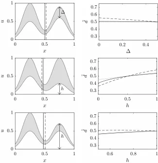
In our first experiment we consider variations of the difference between the upper and the lower memberships. To do so, we set µ1 = 1/4, σ1 = 1/8,

µ2= 3/4,σ2= 1/8,y₁= 0.5,y1= 1,y₂= 0.75−∆/2,y2= 0.75 + ∆/2, where the parameter ∆ is varied in [0,0.5]. The top left graph in Fig. 1 shows an example of this membership function(s) for ∆ = 0.3. Here, the uncertainty of the right Gaussian is a little smaller that the uncertainty of the left Gaussian. The different defuzzification results are marked by vertical lines. In this case, KM (solid) and NT (dotted) yield almost the same results, and UW (dashed) yields a slightly higher defuzzification result which takes into account the fact that the certainty on the right is higher than the certainty on the left. The top right graph in Fig. 1 shows the defuzzification resultsdfor KM, NT, and UW as the uncertainty of the right Gaussian ∆ is changed from 0 to 0.5. For ∆ = 0.5 both Gaussians are equal, and so for reasons of symmetry all three methods yield ˜d= 0.5. As pointed out above, NT (dotted) ignores the different levels of uncertainty and thereforealways yields the output ˜d= 0.5. KM (solid) is only very slightly different from NT (dotted), so here NT is a good approximation of KM with a much lower computational effort. Only UW (dashed) takes into account the (un)certainty and yields a much higher output (closer to the right Gaussian) when the uncertainty of the right Gaussian is lower (for smaller values of ∆).

In our second experiment we consider variations of the lower memberships only, and setµ1= 1/4,σ1= 1/8,µ2= 3/4,σ2= 1/8,y₁= 0.5,y1= 1,y₂=h,

0 0.5 1

x

0.5 1

u

∆

0 0.2 0.4

∆

0.3 0.4 0.5 0.6 0.7

˜

_d

0 0.5 1

x

0.5 1

u

h

0 0.5 1

h

0.4 0.5 0.6 0.7

˜

d

0 0.5 1

x

0.5 1

u

h

0.6 0.8 1

h

0.4 0.5 0.6 0.7

˜

_d

the lower membership function decreases (lowerh), UW (dashed) decreases the result most, then KM (solid), and NT (dotted) decreases the result least. For lower values ofh, i.e. for quite unbalanced uncertainty patterns, KM (solid) and NT (dotted) yield significantly different results. This is an example, where NT does not approximate KM well. As the upper limit of the lower membership function increases (higherh), KM (solid) and NT (dotted) stay almost the same, but UW (dashed) increases the result much more, which reflects the higher certainty of the right Gaussian(s). Forh∈[0.5,1] NT can again be considered a good low effort approximation of KM, but not forh∈[0,0.5], and UW better takes into account the varying uncertainty of the type–2 memberships.

In our third experiment we consider variations of the upper memberships only, and setµ1= 1/4,σ1= 1/8,µ2= 3/4,σ2= 1/8,y₁= 0.5,y1= 1,y₂= 0.5,

y₂=h, where the parameterhis varied in [0.5,1], see the third row of Fig. 1. On the left we see that the maximum upper membership of the right Gaussian is h, here h= 0.7. Also in this case KM (solid vertical line) and NT (dotted vertical line) yield almost the same results, but UW (dashed vertical line) yields a slightly higher result. The right diagram shows the results forh∈[0.5,1]. For

h= 1 we obtain the symmetric case again and all three methods yield ˜d= 0.5. Forh <1 UW (dashed) stays almost constant at ˜d= 0.5, because the reduction of the memberships is approximately compensated by the increased certainty. In contrast to that, KM (solid) and NT (dotted) are almost the same again and decrease with decreasing h. Again, NT is a good approximator for KM, but UW handles the varying uncertainties in an intuitively more reasonable way than KM and NT.

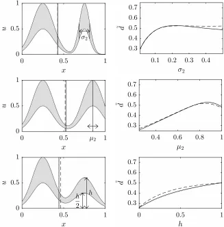
In our second set of experiments we investigate the effect of variations of horizontal widthsσ2, horizontal positionsµ2, and vertical scalesy₂= 2·y₂. In [11, 13] the corresponding transformations are called x–scaling, x–translation, andu–scaling, respectively.

The first row of Fig. 2 shows the effects of variations in the horizontal width

σ2 of the right Gaussian. We set µ1 = 1/4, σ1 = 1/8, µ2 = 3/4, y₁ = 0.5,

y₁= 1,y

2= 0.5,y2= 1 and vary the parameterσ2in [0,0.5]. The left diagram shows the case σ2 = 1/16, where all three methods (solid, dotted, and dashed vertical lines) yield almost the same results. The right diagram shows the results of the three defuzzification methods forσ2= [0,0.5]. Forσ2= 1/8 we have the symmetric case and all three methods yield ˜d = 0.5. For smallerσ2 all three methods yield almost the same results: As the width of the right Gaussian is decreased, the defuzzification result decreases as well. For smaller σ2 KM (solid) and NT (dotted) yield almost the same results: As the width of the right Gaussian is increased, both Gaussians overlap and the left Gaussian gets larger memberships, so also here the defuzzification result becomes lower. For UW (dashed) the results stays close to ˜d≈0.5 because the increasing memberships of the left Gaussian are approximately compensated by an increasing uncertainty (difference between upper and lower memberships of the left Gaussians). Also here, NT is a good approximator for KM, but UW better take into account the uncertainties.

0 0.5 1

x

0.5 1

u

σ2

0.1 0.2 0.3 0.4

σ

0.3 0.4 0.5 0.6 0.7

˜

d

0 0.5 _µ2 1

x

0.5 1

u

0.4 0.6 0.8 1

µ

0.4 0.5 0.6 0.7

˜

_d

0 0.5 1

x

0.5 1

u

h h

2

0 0.5 1

h

0.4 0.5 0.6 0.7

˜

_d

position µ2 of the right Gaussian. We set µ1 = 1/4, σ1 = 1/8, σ2 = 1/8,

y₁ = 0.5, y1 = 1,y₂ = 0.5,y2 = 1 and vary the parameter µ2 in [0.5,1]. For

µ2 = 0.85 (left diagram) all three methods (solid, dotted, and dashed vertical lines) yield almost the same results. The right diagram shows the results for

µ2= [0.5,1]. Forµ2 = 3/4 we have the symmetric case and all three methods yield ˜d= 0.5. Also for all other values ofµ2= [0.5,1], all three methods yield almost the same results, so in this case both NT and UW are good approximators for KM.

The third row of Fig. 2 shows the effects of variations in the vertical scale of the right Gaussian. In contrast to the experiments in the third row of Fig. 1 we not only scale the upper membership function of the right Gaussian, y₂, but also the lower membership function of the right Gaussian,y

2, but keep the ratio between upper and lower memberships equal to 2, so thaty₂= 2·y₂. This simulates the situation that the first rule fires with strength 1 (yielding the left Gaussian) and the second rule fires with strengthh∈[0,1] (yielding the right Gaussian), so in our experiments we can observe the behavior of the output when a rule fades out (or fades in). We set µ1 = 1/4, σ1 = 1/8, µ2 = 3/4,

σ2 = 1/8, y₁ = 0.5, y1 = 1, y₂ = h/2, y2 = h and vary the parameter h in [0,1]. For h = 0.6 (left diagram) we have y₂ = 0.3 and y2 = 0.6, and KM (solid vertical line) and NT (dotted vertical line) yield very similar results, whereas UW (dashed vertical line) yields a slightly higher result. The right diagram shows the results forh ∈ [0,1]. For h = 1 we obtain the symmetric case and all three methods yield ˜d = 0.5. For h = 0 the second Gaussian disappears and all three methods yield the center of the first Gaussian ˜d= 0.25. The transition between the two extremes h = 0 (first rule completely active and second rule completely inactive) andh= 1 (both rules completely active) simulates a gradual increase of the firing strength of the second rule from zero to one. During this transition all three methods smoothly move from ˜d= 0.25 at

h= 0 to ˜d= 0.5 ath= 1. KM (solid) and NT (dotted) yield almost the same results, but UW (dashed) yields slightly higher values, because the certainty of the right Gaussian is higher than the certainty of the left Gaussian. Here again, NT is a good approximator for KM but UW handles uncertainties in more plausible way.

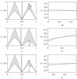
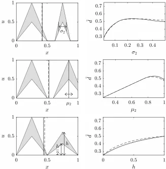
We repeated the same experiments with triangular instead of Gaussian mem-bership functions, where for comparability we chose the triangle widths as 4σ1 and 4σ2.

u(x) = y

1·max

0,1−

x−µ1 2σ1

+y

2·max

0,1−

x−µ2 2σ2

(16)

u(x) = y1·max

0,1−

x−µ1 2σ1

+y2·max

0,1−

x−µ2 2σ2

(17)

0 0.5 1

x

0.5 1

u

∆

0 0.2 0.4

∆

0.3 0.4 0.5 0.6 0.7

˜

_d

0 0.5 1

x

0.5 1

u

h

0 0.5 1

h

0.4 0.5 0.6 0.7

˜

d

0 0.5 1

x

0.5 1

u

h

0.6 0.8 1

h

0.4 0.5 0.6 0.7

˜

_d

0 0.5 1

x

0.5 1

u

σ2

0.1 0.2 0.3 0.4

σ

0.3 0.4 0.5 0.6 0.7

˜

d

0 0.5 _µ2 1

x

0.5 1

u

0.4 0.6 0.8 1

µ

0.4 0.5 0.6 0.7

˜

_d

0 0.5 1

x

0.5 1

u

h h

2

0 0.5 1

h

0.4 0.5 0.6 0.7

˜

_d

2. Again, the results of the triangular case are very similar to the results of the Gaussian case.

6

Conclusions

We have proposed UW, a modification of the NT interval type–2 defuzzifica-tion method that takes into account the uncertainties of the (upper and lower) type–2 membership values. We performed extensive experiments comparing the standard KM method with NT and UW. All experiments were motivated by fuzzy controller scenarios with (for simplicity) two rules, where we inves-tigated the effect of different uncertainty patterns and of different horizontal widths, horizontal positions, and vertical scales of the membership functions on the defuzzification results.

To summarize, our experiments show the following: For the considered sce-narios KM and NT mostly yield very similar results, except when parts of the interval type–2 membership function have very different levels of uncertainty. The computational complexity of KM is much higher than NT. Therefore, NT can often be considered a good approximation of KM with low complexity but only for well balanced uncertainties. UW also has a much lower computational complexity than KM, but in addition explicitly takes into account the uncer-tainty of the interval type–2 memberships, so it yields more reasonable results if more certain decision alternatives should obtain a larger weight than more uncertain alternatives.

This work is a first step in the explicit consideration of uncertainty in type– 2 defuzzification. We have to leave many points open for future research, for example:

• We used the weighting scheme in equation (13) to implement the uncer-tainty weighting, withα= 1. What are other equations or values ofαwill lead to a intuitively plausible treatment of the uncertainties in the type–2 memberships?

• We have applied the uncertainty weighting to the NT method. How could different levels of uncertainty be considered in the KM method?

• How does the behavior of all three methods change if we replace the cen-troid by other (type–1) defuzzification methods?

References

[1] M. Gehrke, C. Walker, and E. Walker. Some comments on interval valued fuzzy sets. International Journal of Intelligent Systems, 11(10):751–759, 1996.

[3] N. N. Karnik and J. M. Mendel. Centroid of a type–2 fuzzy set.Information Sciences, 132:195–220, 2001.

[4] Q. Liang and J. M. Mendel. Interval type–2 fuzzy logic systems: Theory and design. IEEE Transactions on Fuzzy Systems, 8(5):535–550, 2000.

[5] E. H. Mamdani and S. Assilian. An experiment in linguistic synthesis with a fuzzy logic controller. International Journal of Man–Machine Studies, 7(1):1–13, 1975.

[6] J. M. Mendel, R. I. John, and F. Liu. Interval type–2 fuzzy logic systems made simple. IEEE Transactions on Fuzzy Systems, 14(6):808–821, 2006.

[7] M. Nie and W. W. Tan. Towards an efficient type–reduction method for interval type–2 fuzzy logic systems. In IEEE International Conference on Fuzzy Systems, pages 1425–1432, Hong Kong, 2008.

[8] N. Pfluger, J. Yen, and R. Langari. A defuzzification strategy for a fuzzy logic controller employing prohibitive information in command formulation. In IEEE International Conference on Fuzzy Systems, pages 717–723, San Diego, March 1992.

[9] S. Roychowdhury and W. Pedrycz. A survey of defuzzification strategies.

International Journal of Intelligent Systems, 16(6):679–695, 2001.

[10] T. A. Runkler. Selection of appropriate defuzzification methods using appli-cation specific properties. IEEE Transactions on Fuzzy Systems, 5(1):72– 79, 1997.

[11] T. A. Runkler, S. Coupland, and R. John. Properties of interval type– 2 defuzzification operators. In IEEE International Conference on Fuzzy Systems, Istanbul, Turkey, August 2015.

[12] T. A. Runkler, S. Coupland, and R. John. Interval type–2 fuzzy deci-sion making.International Journal of Approximate Reasoning, 80:217–224, 2016.

[13] T. A. Runkler and M. Glesner. A set of axioms for defuzzification strategies — towards a theory of rational defuzzification operators. In IEEE Inter-national Conference on Fuzzy Systems, pages 1161–1166, San Francisco, March 1993.

[14] J. J. Saade and H. B. Diab. Defuzzification techniques for fuzzy controllers.

IEEE Transactions on Systems, Man, and Cybernetics, Part B, 30(1):223– 229, 2000.

[15] L. A. Zadeh. Fuzzy sets. Information and Control, 8:338–353, 1965.