A Bayesian Space-Time Model for Discrete Spread Processes on a Lattice
Long, Jed A.1 [email protected]*
Robertson, Colin2 [email protected] Nathoo, Farouk S.3 [email protected] Nelson, Trisalyn A.1 [email protected] 1
Spatial Pattern Analysis & Research (SPAR) laboratory, Department of Geography, University of Victoria, Victoria, British Columbia, Canada
2
Department of Geography & Environmental Studies, Wilfrid Laurier University, Waterloo, Ontario, Canada
3
Department of Mathematics & Statistics, University of Victoria, Victoria, British Columbia, Canada
*Corresponding Author
Jed A. Long
Department of Geography, University of Victoria PO Box 3060 STN CSC,
Victoria, BC, Canada, V8W 3R4 [email protected]
+1 250 853 3271
Pre-print of published version.
Reference:
Long, JA, C Robertson, FS Nathoo, and TA Nelson. 2012. A Bayesian Space-Time Model for Discrete Spread Processes on a Lattice. Spatial and Spatial-Temporal Epidemiology. 3. 151-162.
DOI:
http://dx.doi.org/10.1016/j.sste.2012.04.008 Disclaimer:
Abstract 1
In this article we present a Bayesian Markov model for investigating environmental spread 2
processes. We formulate a model where the spread of a disease over a heterogeneous landscape 3
through time is represented as a probabilistic function of two processes: local diffusion and 4
random-jump dispersal which allows the model to represent the leptokurtic spread pattern typical 5
of many infectious diseases and biological invasions. We demonstrate the properties of this 6
model using a simulation experiment and an empirical case study – the spread of mountain pine 7
beetle in western Canada. Posterior predictive checking was used to validate the number of 8
newly inhabited regions in each time period. Map comparison analysis was used to measure 9
spatial agreement of spatially distributed model parameter estimates and observed values. The 10
model performed well in the simulation study in which a goodness-of-fit statistic measuring the 11
number of newly inhabited regions in each time interval fell within the 95% posterior predictive 12
credible interval in over 97% of simulations. The map comparison analysis revealed that in some 13
cases the magnitude of estimated parameter values differed markedly from the true values, but in 14
all cases an adequate recovery of the spatial structure was obtained, indicating good spatial 15
agreement. The case study of a mountain pine beetle infestation in Western Canada (1999 to 16
2009) extended the base model in two ways. First, spatial covariates thought to impact the local 17
diffusion parameters, elevation and forest cover, were included in the model. Second, a refined 18
definition for translocation or jump-dispersal based on mountain pine beetle ecology was 19
incorporated improving the fit of the model. Posterior predictive checks on the mountain pine 20
beetle model found that the observed goodness-of-fit test statistic fell within the 95% posterior 21
predictive credible interval for 8 out of 10 years. The simulation study and case study provide 22
evidence that the model presented here is both robust and flexible; and is therefore appropriate 23
for a wide array of spread processes in epidemiology and ecology. 24
25
HIGHLIGHTS 26
Develop and implement a hierarchical Bayes Markov model for spread processes. 27
Case study describing the spread of mountain pine beetle in Western Canada, 1999-2009. 28
Model assessment uses posterior predictive simulation and map comparison statistics. 29
East of Rocky Mountains spread is dominated by translocation events. 30
Model is flexible at handling complex spread processes across heterogeneous landscapes. 31
32
KEYWORDS: space-time binary data, spread process, spatial random effects, mountain pine 33
beetle, map comparison 34
1. Introduction 37
Understanding the emergence and spread of infectious diseases is of increasing concern 38
for promoting global health (Jones et al., 2008). While the reasons for changes in disease 39
patterns over time and space are complex and multidimensional (Morse, 1995), there is a 40
growing need for models capable of describing variation in the spread pattern once cases are 41
being reported (Riley, 2007). Further, understanding underlying risk factors associated with 42
disease amplification is needed to establish appropriate control measures. For example, animal 43
movement and network structure often have an important role in how zoonotic disease epidemics 44
or epizootics develop and spread (Kiss et al., 2006). Similarly in ecology, the spread of non-45
native species are routinely linked to anthropogenic vectors (e.g., Coetzee et al., 2009) or climate 46
change (e.g., Cudmore et al., 2010). As a result, the study of spread processes, defined here as 47
the ability of an organism or disease to expand its current range, is receiving considerable 48
attention in both the epidemiological and ecological literature, and increasingly detailed spatial-49
temporal datasets are providing new opportunities to study the dynamics of spread (see for 50
example, Hooten et al., 2010). Given the increased rate at which many organisms are spreading 51
(Ricciardi, 2007), continued development of methods and tools capable of modeling complex 52
spread processes are warranted. 53
Due to the nature of disease surveillance systems which are the primary data sources for 54
disease modeling studies, data are often only available at discrete temporal intervals (e.g., 55
weeks). Similarly, many pathogens spread via fomites at discrete time periods. For example, 56
marine invasive species such as the zebra mussel (Dreissena polymorpha) spread primarily due 57
to recreational boating, which peaks during the summer months (Schneider et al., 1998). Other 58
disperse on an annual basis (Safranyik & Carroll, 2006). As a result, there is considerable interest 60
in developing discrete-time representations of spread in ecological models. 61
Spatially, data can be represented as either an aggregated spatial unit (i.e., discrete) or as 62
point-events (i.e., continuous). For most ecological models, aggregated data are used simply due 63
to ease of field sampling. Units are analogous to quadrats in which the presence / absence or 64
abundance of the species is measured. While continuous spatial data provide a high level of 65
spatial detail, this is typically purchased at the expense of the spatial extent of the study. For 66
ecological models at the landscape scale, point-event data are often not feasible. For both 67
discrete and continuous spatial data, representation of landscape heterogeneity is often a major 68
limitation in models of spread (Pitt et al., 2009). For example, physical barriers such as 69
mountains and rivers are often poorly represented using traditional geographic data formats 70
(Cova and Goodchild, 2002). This issue is exacerbated by the fact that processes at multiple 71
spatial scales act in concert to produce spread patterns on the landscape, yet modeling is often 72
carried out at a single spatial scale (Pitt et al., 2009). Pearson and Dawson (2003) have proposed 73
hierarchical modeling as a potential solution which can incorporate ecological mechanisms at 74
multiple spatial scales. 75
The spread of disease is often the result of multiple mechanisms. For example, foot and 76
mouth disease typically spreads among animals and herds via airborne transmission, and among 77
farms and regions by animal movement networks and fomites (Green et al., 2006). Similarly, in 78
many ecological invasions, the resultant pattern of invasion is often multi-causal: locally through 79
diffusion or movement and over greater distances via intermediate species or translocation 80
vectors. Smith et al. (2002) provide a mathematical model for spread processes characterized by 81
lattice in their example. However, inference in Smith et al. (2002) was based on a stochastic 83
estimation algorithm rather than a formal statistical framework for inference. The spread of 84
raccoon rabies was also examined by Wheeler and Waller (2008) who link spatial variation in 85
patterns of spread (i.e., deviations from a travelling wave) to landscape heterogeneity using 86
spatially-varying regression, and adopt a Bayesian framework for inference. 87
Bayesian space-time spread models have previously been formulated for investigating 88
environmental spread processes with point-referenced count data, (e.g., Wikle, 2003; Hooten and 89
Wikle, 2006). As well, Gibson et al. (2006) have developed a Bayesian space-time percolation 90
model for contact-based (local) spread across a spatial lattice; however, the model developed 91
there does not accommodate translocation events, where the disease process spreads across 92
disconnected regions. This is particularly important considering that the broad scale outcomes of 93
spread by many ecological organisms are dominated by random-jump translocation events, and 94
not local diffusion (e.g., Suarez et al., 2001). 95
Despite the inherent link between the spread of species of interest to ecologists, and 96
disease spread in human populations studied by epidemiologists, models have been developed 97
largely independently in these fields until very recently (Smith et al., 2002). Given that the 98
majority of emerging diseases are zoonotic in nature (Jones et al., 2008), and often of wildlife 99
origin, there exists a need for integrated ecological-epidemiological modeling. In this article we 100
present a hierarchical Bayes approach appropriate for modeling either disease or organism spread 101
across a landscape, and allow for landscape heterogeneity using spatially-varying parameters. 102
Although we investigate a specific ecological application (i.e., mountain pine beetle in western 103
Canada), the methods employed are generic and appropriate for a wide range of spread problems 104
In this article, we present a discrete-time Markov model for ecological spread processes 106
allowing for spatially-varying spread rates and random-jump dispersal. In the next section we 107
present the model. A simulation study follows, which evaluates model performance. Simulated 108
datasets at multiple spatial scales, under various spread scenarios, are used to illustrate model 109
strengths and weaknesses. Next, we report on an empirical case study investigating the spread of 110
mountain pine beetle (Dendroctonus ponderosae) in western Canada. Finally, we discuss 111
remaining challenges and practical issues related to the process of model development and 112
conclude by linking this research with potential applications in epidemiology. 113
2. Model Development 114
Given n regions comprising a study area, we formulated a logistic model for a binary 115
spread process (defined here as inhabited-uninhabited) where it was assumed that newly 116
inhabited regions do not revert to being uninhabited (Mollison, 1977), and we 117
letZi(t){0,1}indicate the presence of an organism or disease in region i, i=1,…, n, at time t,
118
t=1,…,T. Here, t = 1 corresponds to the initial map of organism or disease presence, and the 119
vector Z(t) = (Z1(t), …, Zn(t))' represents a binary map describing the progression of the 120
organism or disease at time t. Spread is described through a stochastic process model for Z(t), 121
which conditional on model parameters Θ, is assumed to follow a first-order Markov 122
assumption, so that 123
Pr{Z(t)|Z(t-1),Z(t-2),…,Z(1),Θ} = Pr{Z(t)|Z(t-1),Θ} where the Markov transition kernel is 124
indexed by Θ. The Markov model is further simplified by assuming conditional independence 125
across regions, so that 126
Pr{Z(t)|Z(t-1),Θ} = Πi Pr{Zi(t)|Z(t-1),Θ}. Spatial dependence is accommodated at the second 127
level of the hierarchical specification with random effects incorporated into Θ. The term pit =
Pr{Zi(t)|Z(t-1),Θ} represents the probability that the organism or disease is present in region i at 129
time t, given the presence map Z(t-1) and conditional on Θ. We assumed that regions where the 130
organism or disease is present remain inhabitated, so that pit = 1 if Zi(t-1) = 1; whereas, if region 131
i is free of organism or disease at time t-1, so that Zi(t-1) = 0, we assumed a logistic specification
132
with space varying coefficients 133
log{pit /(1- pit)} = μt + λi NN[i,t-1] [1] 134
where NN[i,t-1] is the number of inhabited neighbors of region i at time t-1; μt is a time varying
135
parameter representing a baseline probability of becoming inhabited; and λi is a spatially-varying 136
parameter quantifying the local impact of inhabited regions on their uninhabited neighbors. 137
Neighbors for NN[i,t-1] are defined using a Queen’s case (Moore neighborhood – i.e., edge or 138
corner in contact signifies a neighbor) definition of spatial neighbors; however, alternate 139
neighborhood configurations could easily be explored. The baseline rate μt is common to all 140
regions, and for an uninhabited region with no inhabited neighbors at time t-1 (isolated from the 141
spread wave) we have 142
log{pit /(1- pit)} = μt [2] 143
so that μt can be thought of as representing the time-varying probability of translocation events, 144
describing random-jump movements by a species. Inclusion of terms for both diffusion and 145
random-jump movements is important when spread occurs via separate mechanisms or at 146
differing spatial scales. Mountain pine beetles, for example, spread via two independent 147
mechanisms, actively over short distances (e.g., within forest stands), and passively via 148
convective wind currents capable of transporting small populations for hundreds of kilometers 149
Comparison of equations [1] and [2] reveals that λi characterizes the change in the log-151
odds of habitation for region i, arising from the presence of organisms in neighboring regions. 152
Larger values of λi correspond to an increasing probability of spread from inhabited regions to 153
uninhabited neighbors. As such, λi controls the rate of organism mobility or diffusion into region
154
i, and the vector λ = (λ1,…, λn)' characterizes spatial variability in diffusion across the entire 155
study area. 156
Using a hierarchical modeling approach, we allowed for temporal variation in the 157
translocation parameters μ = (μ1,…, μT)' and spatial variation in diffusion parameters λ = (λ1,…,
158
λn)' using mixed model random effect specifications. The translocation component μ, is
159
composed of a constant μc, coupled with time-varying mean-zero effects θt, so that 160
t c
t
[3] 161
A weakly informative prior for μc was adopted, using a Normal distribution with mean 0 and a 162
precision of 1/1000, or μc ~ N(0,0.001). The θt represent year-to-year variation in translocation,
163
and are modeled independently as θt ~ N(0,τθ) with the variance τθ assigned a conditionally 164
conjugate inverse-Gamma hyper-prior τθ ~ inverse-gamma(0.01,0.01). 165
The spatially-varying diffusion parameters λ = (λ1,…, λn)' are modeled using a
166
convolution prior 167
i i
i 0 h a
[4]
168
where α0 represents the baseline level of spread across the study area; hi ~ N(0,τh) are 169
independent and identically distributed random effects representing spatially unstructured 170
variation; and ai is a spatially correlated random effect, with the vector a = (a1,…, an)' modeled 171
using an intrinsic conditional autoregressive model – CAR(τa). This random effect formulation 172
correlated random effects.. Additional terms corresponding to spatially varying covariates can be 174
easily incorporated in [4] to investigate relationships between covariates and the local rate of 175
diffusion. The spatial CAR model for ai uses a Queen’s case (i.e., adjacency) definition of 176
neighbors. In addition, a binary definition of weights is used, with neighbors coded as 1 and non-177
neighbors as 0. Finally, our model specification is made complete by assigning a flat prior to α0, 178
and weakly informative inverse-gamma(0.5,0.0005) hyper-priors for the variance components τh 179
and τa. 180
The vector Θ is the set of parameters in our model, with Θ = {h, a, θ, α0, μc, τα, τh, τθ}. 181
With this specification, Bayesian inference for Θ is based on the posterior distribution 182
[Θ|Z(1),…,Z(T)], where Z(1),…,Z(T) are binary data vectors representing a realized ecological 183
spread process. The posterior distribution is computed using Markov chain Monte Carlo methods 184
implemented in the free software WinBUGS (Lunn et al., 2000). The model code used for fitting 185
this model can be obtained from the first author upon request. 186
187
3. Model Evaluation Using a Simulation Study 188
3.1 Simulation Study Data
189
We carried out a simulation study to assess the model performance under different 190
scenarios describing the spread of disease. While employing Bayesian inference to ‘borrow 191
strength’ can help address the issue of inaccurate estimation due to infrequent sampling (i.e., big 192
area; small numbers), the opposite effect may be true for pooled estimates that are pulled too 193
much towards the mean (Gelman and Price, 1999). When applied with real data the diffusion 194
simulation-estimation approach to investigate the sensitivity of the model to changes in model 196
parameter values and spatial scale. 197
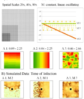
Spread datasets were simulated from a set of patterns representing realistic scenarios of 198
spatial diffusion (Figure #a) and time-varying translocation (Figure #b), in combination with 199
three different spatial scales. Spatial diffusion represented as a linear trend (Λ1) can be thought to 200
represent a simplified spread process across a more homogeneous landscape, this scenario might 201
be encountered, for example, in the presence of a latitudinal gradient. The Gaussian random field 202
scenario (Λ2) is an example of a more complex, heterogeneous landscape, characteristic of a 203
wide range of spread processes. Constant translocation (M1) represents a static level of random 204
translocation events. Linear decreasing translocation (M2) represents a situation where a spread 205
mechanism (e.g., fomite transmission of foot and mouth disease) is decreasing over time as 206
control measures are put in place. Finally, oscillating translocation (M3) represents a seasonal 207
cycle to translocation, as in the case of wind-driven transport which depends primarily on 208
seasons. Variation in spatial scale (20x20, n = 400; 40x40, n = 1600; 80x80, n = 6400) is used to 209
examine the impact of scale on model performance. Specifically, we are interested in how 210
changes in the grain (resolution) of the data may affect results. Extent, the other aspect of spatial 211
scale, is of less interest here, as we assume the extent of the disease is contained by the study 212
area. 213
< approximate location for Figure #a,b >The simulation-estimation procedure involved 214
three steps: 1) generate a realistic spread scenarios using combinations of diffusion (Λ), 215
translocation (M), and spatial scale (see Figure #); 2) simulate spread data from the scenarios; 216
and 3) estimate the model based on the simulated data. Each combination of spatial diffusion 217
total of 18 different scenarios (the simulated spread datasets for the 6 scenarios at the 40x40 219
scale are shown in Figure ##). 220
< approximate location for Figure ## > 221
3.2 Examining Model Fit
222
To compare the true and estimated diffusion values we used a global chi-square goodness 223
of fit statistic where bins were set at intervals of 0.25. The test is a comparison of the number of 224
observations in each bin for the known parameters and the number of estimates in each bin in the 225
estimated parameters. In addition to chi-square tests, we also report standardized residuals for 226
both diffusion and translocation, defined as the absolute value of the difference between the true 227
and estimated parameter value, divided by the number of observations (n for diffusion, T-1 for 228
translocation). 229
To evaluate model fit to the simulated data, we used posterior predictive checking 230
(Gelman et al.,2004). To perform posterior predictive checks, 100 draws from the posterior 231
distribution of all diffusion and translocation parameters were obtained. Data were simulated 232
with the model using these parameter values to create 100 replicate datasets from the posterior 233
predictive distribution. We assessed similarity between these replicates and the observed data for 234
some test quantity of interest (Gelman et al.,2004). In our case the observed data are the original 235
data used to describe a spread process, and were generated by the model using the chosen 236
parameter values, while in practical applications this would be the observed spread data. The test 237
statistic we used was the number of new cells inhabited in each time period, Inht, where 238
n i i it Z t Z t
Inh 1 ) 1 ( )
( [5]
239
Two of the simulated datasets were selected for checking based on the results of the parameter 240
performing scenarios were evaluated, both using the 40x40 spatial scale to ensure comparability. 242
In each case the test statistic was evaluated at each time point to determine if a value of Inht
243
computed for the data falls outside the main mass of the corresponding posterior predictive 244
distribution, in which case we have evidence that the model does not fit this aspect of the data. 245
We also examined the spatial structure of local diffusion using map comparison analysis. 246
The objective of map comparison is to uncover similarities (or differences) between expected 247
(Λ) and estimated (λ) diffusion maps, and evaluate whether two maps could have been generated 248
by the same process. This is facilitated in the simulation examples as we have both an expected 249
diffusion map (e.g., those Λ in Figure 2 from which the spread process was generated) that we 250
can compare to the mean posterior predictive estimates (λ). In terms of model validation, 251
considering spatial structure provides improved confidence in estimated λ over purely aspatial 252
comparisons. The structural similarity (SSIM) index was selected as an exploratory statistic for 253
comparing maps (Wang et al.,2004). SSIM incorporates a Gaussian weighting function, to 254
assess similarity across spatially local regions. This is in contrast to direct pixel to pixel 255
comparisons, which ignore spatial structure in maps, often producing comparison measures 256
highly sensitive to slight spatial misalignment (Pontius Jr., 2000). SSIM considers three 257
components for map comparison: luminance, contrast, and structure, relating to local differences 258
in mean, variance and covariance respectively (Wang et al.,2004). Note that these three 259
components are relatively independent, and changes in one component will not necessarily affect 260
others. SSIM takes the following spatially local form, computing a similarity statistic for each 261 spatial unit: 262 )] ( [ )] ( [ )] ( [ )
(i l i c i s i
SSIM [6]
where i denotes the ith spatial unit, l the luminance component, c the contrast component, and s
264
the structure component (see Wang et al.,2004 for further details). The exponents α, β, and γ can 265
be used to weight individual components, with default values taken as α = β = γ = 1. The local 266
components l(i) and c(i) are strictly positive while s(i) can take on negative values. We report 267
only the mean global statistic for each of the three components and overall similarity, noting that 268
although locally the product from [6] holds, due to summation rules the mean SSIM value does 269
not equal the product of the means of each component. When two maps are identical, SSIM = 1, 270
and values decrease from 1 as similarity decreases. SSIM was calculated for all 6 simulated 271
scenarios at the 40x40 spatial scale. Given the map size (40x40), we selected a Gaussian 272
weighting function with parameters h = 3 and sd = 0.5. SSIM results were insensitive to minor 273
changes to h and sd. 274
As a final check on model sensitivity, we varied the hyper-parameters corresponding to 275
the prior variances for random effects governing variation in both diffusion and translocation to 276
other suggested alternatives, inverse-gamma(0.001, 0.001) and inverse-gamma(0.1, 0.1). The 277
effects of these prior adjustments on point estimates for diffusion and translocation are reported. 278
3.3. Simulation Study Results
279
The global goodness of fit analysis for the 27 different simulated spread scenarios are 280
reported in Table #. These global chi-square tests reveal that in none of the scenarios were the 281
estimated parameters significantly different than the true values. The standardized residuals 282
demonstrate the effects of changes in the pattern of spread and spatial scale on diffusion 283
(Appendix B). Residuals tended to increase with larger study areas. For the 20x20 and 40x40 284
spatial scales, the Λ2 spatial trend produced larger error than the Λ1 spatial trend or the Λ3 285
study area. For translocation, the opposite general pattern holds, with larger residuals for smaller 287
datasets. This is likely due to the lack of available cells for translocation to occur at smaller 288
scales. The interdependency between diffusion and translocation is illustrated in Appendix B. 289
Interdependency is clearly impacted by spatial scale, with fairly similar patterns in residuals at 290
the 20x20 scale, and less so at larger scales. 291
< approximate location for Table # > 292
Analysis of model fit using posterior predictive checks based on the statistic Inht is
293
presented in Figure 5. For datasets simulated from scenario Λ2Μ3 and scenario Λ3Μ2, the test 294
statistic fell within the 2.5 and 97.5 percentiles (95% credible interval), 97 and 98 times (out of 295
100) respectively, indicating a very good fit to the data. For the simulated data, the model 296
appears to capture the timing of newly inhabited cells well. 297
< approximate location for Figure 5 > 298
Map comparison of estimated (λ) and expected (Λ) diffusion maps (40x40 spatial scale) 299
revealed different trends from purely aspatial measures reported in Table ##. Estimated λ maps 300
associated with Μ2 showed the lowest similarity in all three Λ scenarios. In the case of scenarios 301
Λ1Μ2 and Λ2Μ2, mean SSIM values were extremely low (-0.026 and 0.064 respectively) 302
indicating poor model fit. These low SSIM values can be attributed to low scores in the 303
luminance component (0.231 and 0.214 respectively). Map similarity was considerably higher in 304
the other scenarios, with a maximum of 0.754 for scenario Λ1Μ1. 305
< approximate location for Table ## > 306
Finally, model sensitivity to hyper-priors on variance parameters of the spatial CAR 307
component (τa) revealed the model inference to be robust to the prior forms considered. Effects 308
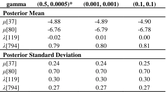
Table 2. For both diffusion and translocation, changes in parameter estimates ranged from 0 to 310
0.03 for posterior means, and 0 to 0.02 for posterior standard deviations. 311
< approximate location for Table 2 > 312
Overall, the simulation study provides convincing evidence that the model and the 313
corresponding Bayesian inference are able to recover the parameter values used to simulate the 314
data. Changes to variance hyper-parameters for diffusion and translocation have little impact on 315
estimation in the settings we considered. Further, the effect of spatial scale has also been shown 316
to be an important consideration. Highlighted by map comparison analysis, spatial structure does 317
indeed play an important role in assessment of maps of true vs. estimated output parameters. 318
Map comparison revealed that when maps of true (Λ) vs. estimated (λ) diffusion parameters were 319
dissimilar the bulk of this difference can be attributed to the magnitude of the values 320
(luminance), and that our model does effectively reveal expected spatial structure. This means 321
that in some cases interpretation should be limited to spatial patterns observed, taking the 322
magnitude of reported λ values as potentially misleading. In many cases modeling efforts 323
primarily investigate spatial patterns of output parameters (e.g., high areas vs. low areas), and 324
less so the magnitudes of output values. The model is effective at identifying such spatial 325
variation in parameter estimates. 326
4. Empirical Case Study – Mountain Pine Beetle in Western Canada 327
4.1. Background
328
Mountain pine beetle is the most destructive biotic agent of mature pine forests in 329
western North America (Safranyik & Carroll, 2006). Endemic to this region, mountain pine 330
beetles typically attack weakened pine trees scattered throughout the forest. Periodically, when 331
causing mortality to mature pine trees covering thousands of hectares (Safranyik & Carroll, 333
2006). Originating around 1998, the current outbreak is the largest on record and has devastated 334
western Canada’s forest industry, causing substantial timber losses (British Columbia Ministry of 335
Forests and Range, 2007). A warming climate combined with forest fire suppression has resulted 336
in an overabundance of mature lodgepole pine (Pinus contorta) trees on the landscape. As 337
lodgepole pine are the preferred host of mountain pine beetle, the combined effect of a warming 338
climate and forest fire suppression is listed as probable cause for the magnitude of the current 339
outbreak (Carroll et al.,2006). 340
The historical range of mountain pine beetle in Canada is predominantly within the 341
province of British Columbia (Figure 3). Current epidemic mountain pine beetle populations 342
have breached historic physiographic (e.g., Rocky Mountains) and climatic barriers to spread 343
(Safranyik et al.,2010). Substantial beetle populations now exist in the province of Alberta, 344
where the range of the beetles preferred host – lodgepole pine, meets the range of jack pine 345
(Pinus banksiana) (Figure 3). Empirical evidence has found that jack pine is an alternative 346
suitable host for mountain pine beetle (Furniss and Schenk, 1969; Cerezke, 1995). In the absence 347
of climatic factors inhibiting beetle populations, jack pine, present throughout the boreal forest, 348
could provide continuous habitat facilitating further eastward expansion by mountain pine beetle 349
and negative economic and ecological consequences in Canada’s boreal region (Logan and 350
Powell, 2001; Carroll et al., 2006; Safranyik et al., 2010). 351
< approximate location for Figure 3 > 352
The objective of this case study is to use the proposed Bayesian spread model to learn 353
about processes governing the spread of mountain pine beetle at the boundary of its historical 354
facilitate movement of beetle populations. Active spread represents spatially local dispersal 356
events where beetles fly within or between neighboring pine stands and is the principle mode of 357
spread (Safranyik et al.,1992). Mountain pine beetles are also capable of passive spread whereby 358
beetles are carried long distances via convective wind currents during periods of emergence 359
(Shepherd, 1966; Furniss and Furniss, 1972; Ainslie and Jackson, 2011) . The model we have 360
developed captures active spread through the spatially local diffusion parameters – λ, and passive 361
spread through the temporally stochastic translocation parameters – μ. We hope to gain insight 362
into mountain pine beetle spread during the current epidemic by interpreting spatial variation in 363
λ, and temporal variation in μ. 364
4.2. Data and Study Area
365
Mountain pine beetle infestation data were obtained from the British Columbia Ministry 366
of Forests and Range1 and the Alberta Department of Sustainable Resource Development2 for 367
each year of our study (1999 – 2009). These infestation data are primarily obtained through 368
aerial overview surveys, but also in situ measurements and remotely sensed data sources. 369
Mountain pine beetle emergence occurs during a short one month window during the summer in 370
the study area. As such, the spread process can be measured at discrete (i.e., annual) intervals. 371
Infestation events are represented as both points (indicating a small cluster of infested trees) and 372
polygons (a large area of infestation). 373
We selected a rectangular study area that covers the northern portion of the eastward 374
expansion by mountain pine beetle into the province of Alberta (inset Figure 3). A 12 km grid 375
was demarcated across the study area, generating n = 2310 contiguous spatial units. Similar 12 376
km spatial units have been used for investigating characteristics of a previous mountain pine 377
1 More Info at: http://www.for.gov.bc.ca/hfp/health/overview/overview.htm
beetle outbreak in British Columbia (Aukema et al., 2008; Zhu et al., 2008) and spatial 378
synchrony within the current outbreak (Aukema et al., 2006). 379
We were also interested in investigating relationships between mountain pine beetle 380
spread (Figure 4a) and environmental factors. Two spatial covariates, elevation and forest cover 381
(see Figure 4 b and c), were identified in the literature as important in governing local spread of 382
mountain pine beetle. Elevation was taken as the mean of elevation values within each spatial 383
unit using a fine grain elevation dataset (spatial resolution of 25 m). Percent forest cover for each 384
spatial unit was determined using a national land cover database (Wulder et al., 2008). These 385
spatial covariates were incorporated into the model for λ [4], and relate to local diffusion so that 386
[4] becomes 387
i i i
i X h a
0 [7]
388
where Xi is a vector of spatial covariates (e.g., elevation, percent forest cover) at location i, and β 389
are the associated coefficients. 390
< approximate location for Figure 4 > 391
Exploratory spatial analysis revealed that mountain pine beetle translocation events 392
exhibited distance-dependence, whereby translocation events occur more frequently proximal to 393
previously infested regions. This phenomenon is commonly associated with the characteristic 394
leptokurtic pattern of spread (e.g., in animal-borne diseases #Fergusan, Lindstrom#, human 395
diseases #REF#, and with invading organisms, Lewis 1997) whereby translocation events are 396
distance-dependent relative to the spread wave. . In this scenario, extremely long distance 397
translocation events are rare, but still possible. To account for this effect, we considered a more 398
general model for the translocation component that more appropriately resembles this distance-399
t it c
it d
~ [8]
401
where ~it is a spatial and temporally varying translocation parameter, d
it is the distance (centroid
402
to centroid) from cell i to the nearest infested region at time t, with coefficient γ, and μc and θt are 403
as defined in [3]. This treats the distance values (dit) as a space-time covariate modulating the 404
translocation component. 405
4.3. Model Implementation
406
Several variations of the model were implemented incorporating different parameters 407
(Table 1). For each model, two MCMC chains were run to fit the model. Convergence was 408
assessed following Brooks and Gelman (1998), and a conservative burn-in of 10 000 iterations 409
was selected. Following burn-in, 20 000 samples from each chain were retained for inference. 410
Model selection was based on the deviance information criterion (DIC), which combines the 411
deviance with a penalty for model complexity (Spiegelhalter et al.,2002). Posterior mean, 412
variance, and 95% equal-tailed credible intervals were used to summarize the posterior 413
distributions. 414
< approximate location for Table 1 >4.4. Case Study Results
415
Variation in DIC between model 1 and 2 was substantial, indicating that the inclusion of 416
a distance-dependent translocation term (it
~ from [8]) improved the model (see Table 1). As
417
such, the four subsequent model specifications all use the ~it definition from [8]. The variation
418
in DIC between models that use the it
~ definition for translocation (models 2 – 6) was small
419
(Table 1). The addition of the aspatial random effect parameter (h) had little effect on the DIC. 420
However we include h in subsequent model specifications as it can be used to interpret variation 421
in mountain pine beetle spread not captured by the smoothing effect of the CAR model and/or λ 422
(including both the elevation and forest cover covariates) resulted in the lowest DIC value, and 424
forms the basis for further discussion. 425
To evaluate model fit we performed a posterior predictive check similar to that described 426
in the simulation experiment. For the case study data, we drew 1000 samples from the posterior 427
distribution of each parameter and these were then used to draw 1000 replicate datsests (Zrep) 428
from the posterior predictive distribution. The test statistic (inht – see [5]) of the true infestation 429
data fell within the 2.5 and 97.5 percentiles (95% posterior predictive credible interval) of the 430
simulated Zrep data in all but two years (8 out of 10), indicating a reasonable model fit (Figure 6).
431
The two anomalies were associated with the first year after initial infestation (2000) and an 432
extreme peak in infestations that occurred in 2007. 433
< approximate location for Figure 6 > 434
A negative relationship (posterior mean = -0.153, 95% C.I. = [-0.337, 0.019]) was 435
observed between local diffusion rate and the elevation covariate. A negative relationship 436
between mountain pine beetle and elevation in British Columbia has been previously reported, 437
and is believed to be linked to elevational constraints on pine species, the beetles preferred host 438
(Aukema et al., 2008; Zhu et al., 2008). This relationship does not necessarily apply east of the 439
Rocky Mountains and may be reason that this relationship is rather weak (e.g., the 95% credible 440
interval covers zero). The rugged topography of the Rocky Mountains historically provided a 441
physical barrier to eastward expansion by mountain pine beetle, with only a few small cases of 442
infestation observed east of the Rockies (see Cerezke, 1989). The current epidemic has breached 443
this barrier, and continued eastward expansion by mountain pine beetle through the boreal will 444
A positive relationship (posterior mean = 0.2681, 95% C.I. = [0.130, 0.406]) was 446
identified between local diffusion rate and forest cover. In British Columbia, elevation had 447
previously been used as a surrogate for forest cover information, as here lodgepole pine is found 448
primarily at lower elevations. As previously mentioned, east of British Columbia topography is 449
far less variable, and pine species are found throughout the range of elevations within the boreal 450
forest. As mountain pine beetle continues its eastward expansion, variables that more 451
appropriately represent the availability of suitable pine hosts directly will be most useful for 452
predicting infestation. 453
Using a map of the spatially-varying diffusion parameter (λ) we can highlight regional 454
variability in the rate of local spread (Figure 7a). Comparing to the time of infestation map 455
(Figure 4a) we can clearly see that high λ values are found immediately east of the originally 456
infested regions. Here due to the rugged topography, mountain pine beetle spread quickly along 457
linear forest tracts in valley bottoms as has been previously demonstrated (Robertsonet al., 458
2009). Caution should be taken interpreting λ values in regions where no infestation has occurred 459
(such as in the most eastern portion of our study area). Here the model infers a continuous λ 460
surface from few relevant λ measurements and posterior variance is highest (Figure 7d). 461
< approximate location for Figure 7 > 462
The map of the aspatial random effect parameters (h), can be used to identify regions 463
where the smoothing of the CAR effect (Figure 7b) over-estimates (negative values) or under-464
estimates (positive values) the rate of local diffusion (Figure 7c). Regions over-estimated 465
(negative values in Figure 7c) by the CAR portion of the model are likely due to abrupt changes 466
in land cover resistant to mountain pine beetle (such as large lakes or mountain peaks). This 467
representation of barriers is discrete rather than continuous. Reason for areas under-estimated 469
(positive values in Figure 7c) may be due to the topographic effect mentioned earlier. However, 470
the magnitude of the h effects are quite small (-0.007 to 0.005). Given that the h effect is quite 471
small, the λ maps are therefore predominantly associated with a combination of the CAR effect 472
(a) and the environmental covariates (Xβ). 473
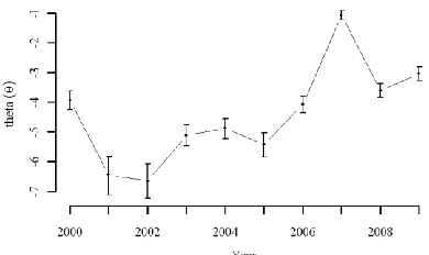
We also examine annual changes in translocation (it
~ ) through time, by way of the
474
parameter θt. Mountain pine beetle translocation is highest in 2007, identified by the sharp peak 475
in θt values in that year (Figure 8). In this example, interpretation of temporal trends in θt 476
requires consideration of original mountain pine beetle infestation data sources. Aerial overview 477
surveys and remotely sensed data rely on visual cues of tree mortality (i.e., foliage turning red), 478
which occurs 1-2 years after beetle presence. Thus, the peak value of θt observed in 2007 479
actually corresponds to increased translocation events by mountain pine beetle in 2005 or 2006. 480
This is in line with reports of extensive beetle activity in 2006 (Carroll, 2010). Although 481
temporal climate covariates were not investigated here, factors such as uncharacteristically warm 482
summers or cold winters influence beetle populations, and the success of the beetles passive 483
spread mechanism (Stahl et al., 2006). 484
< approximate location for Figure 8 > 485
With some ecological invasions, barriers may be introduced as a management tactic, 486
effective at slowing the spread of an invading species (Sharov and Liebhold, 1998). In Western 487
Canada, clear-cut harvests and controlled forest fires have been implemented as barriers to 488
mountain pine beetle spread through the removal of large, contiguous sections of potential host 489
trees. In British Columbia, the voracity of the current epidemic has circumvented any mitigation 490
measures will prove successful at stopping future eastward beetle spread. Preventing continued 492
expansion by mountain pine beetle will be challenging given evidence that the beetles 493
reproductive success improves in lodgepole pine stands outside of its historical range (Cudmore 494
et al.,2010). Further, from our analysis it is clear that east of the Rocky mountains, mountain 495
pine beetle spread, like many other spread processes (e.g., Suarez et al., 2001), is dominated by 496
translocation events. When translocation dominates ecological invasions, the organism is often 497
able to jump spread barriers rendering them ineffective. In such cases, it is necessary to carefully 498
evaluate whether the introduction of barriers will provide the intended ecosystem and economic 499
benefits (Sharov and Liebhold, 1998). 500
501
5. Discussion & Conclusions 502
503
The validation process we adopt is an example of how both aspatial and spatial indices 504
can be incorporated into the validation procedure. Following guidelines of Gelman et al.(2004), 505
we use posterior predictive checking as an aspatial measure of model fit that can be used even 506
when true parameter values are unknown. This posterior predictive check revealed that our 507
model is sufficient at recovering the timing of new infections. In the simulation study, we were 508
able to complement this aspatial technique with a map comparison analysis (SSIM - Wang et al., 509
2004) to assess spatial structure of λ values. Map comparison analysis revealed that in some 510
cases estimated λ values were different from expected in magnitude, but that in general the 511
spatial pattern of λ values was retrieved. The SSIM method enables creation of maps of local 512
differences in mean, variance, and covariance, providing information on the spatial structure and 513
approach to model evaluation represents a relatively simple procedure that can be easily 515
implemented with existing models providing valuable and unique insight on how spatial 516
structure of parameters relate to model performance. The SSIM measure was originally designed 517
for evaluating image compression algorithms, and only recently has been proposed as a useful 518
measure for quantitative comparison of continuous-value maps #Hagen-Zanker#. Thus, 519
improving our understanding of how the SSIM (or other similar statistics) can be used as spatial 520
measures of model evaluation remains an ongoing endeavor. . 521
Both in the simulation examples and the case study we model spread across a regular 522
tessellation (grid). In the mountain pine beetle example, we selected 12 km units as spatial unit 523
for which to model spread. Our analysis was undoubtedly impacted by this selection, but also, by 524
the scales at which the infestation and covariate data were collected. In the context of 525
epidemiological spread models, how the at-risk population, the environment, , and population-526
environment interaction are represented will undoubtedly impact results. The use of regular 527
and/or square spatial units are not required, and as in Smith et al. (2002) an irregular lattice (such 528
as counties) could be appropriately used with this model. The implementation of an irregular 529
lattice map structure would require careful consideration to the definition of spatial weights. For 530
example, it may be useful to consider the proportion of the boundary associated with infected 531
polygons surrounding an uninfected region as a way to accommodate the spatial structure of 532
infected neighbors in [4]. Alternatively, higher-order spatial weights functions (e.g., using a 533
distance-decay effect) may be useful for quantifying disease pressure in uninfected regions 534
#REF#. 535
Working within a hierarchical Bayesian framework allows for data at multiple 536
Bayes framework is used as a security blanket when tasked with modeling erroneous or sparse 538
datasets. However, inferences resulting from such analyses are still a product of limited datasets 539
(i.e., garbage in – garbage out). Thus care must be taken to utilize a hierarchical Bayes 540
framework in such a way as to maximize the potential learning from available data, while 541
recognizing the limitations of a given dataset. The flexibility of the model presented here, from 542
the basic structure introduced in section 2 to the more complex variations used in the mountain 543
pine beetle example, and further proposed in the discussion, can provide an accommodating 544
framework for modeling many characteristic dual-mechanism (diffusion-translocation) spread 545
processes.. A key feature of the proposed model is the incorporation of spatially-varying 546
diffusion parameters, which allow for local differences in rates of spread across the study region, 547
accommodating diffusion across heterogeneous landscapes. Incorporating spatially varying 548
parameter values into a model framework (for example using geographically weighted regression 549
#Fotheringham# or, more broadly, any spatially varying coefficient model #e.g.,Waller et al. 550
2007#) is becoming increasingly popular for examining spatial heterogeneity in a wide range of 551
applications, for example disease mapping (Best et al. 2005), crime rates, (Wheeler and Waller 552
2009), and housing values (Bitter et al. 2007). The additional complexity of varying parameters 553
over space is no longer a computational burden given modern computing capabilities, and 554
resulting maps of parameter estimates, such as those in Figure 7, can provide material for 555
interesting spatially-specific inference. However, it can be easy to attempt increasingly complex 556
models beyond what is capable of being learned from the data (i.e., over-fitting). This can lead to 557
a variety of problems including high parameter variance and sensitivity #REF#, and poor overall 558
fit. It is up to the researcher to determine what can be realistically learned from the data with 559
Here, using a convolution model for the diffusion process, we examined spatially 561
structured (a) and non-structured (h) error terms (e.g., following the BYM model, Besag, York, 562
and Mollie 1991). In theory, maps of the non-structured term could be linked to spread barriers, 563
although in this example the effect was relatively small in magnitude. In ecological examples, 564
barriers are often a function of physical properties of the landscape (Sharov and Liebhold 1998). 565
However in epidemiology, where infections are commonly transferred along networks, the 566
identification of barriers will be more complex as they are related to the connectivity of infected 567
and susceptible nodes (Eubank et al. 2004, Keeling 2005). The identification and interpretation 568
of various anomalies (e.g., barriers) within maps of spatially varying parameter estimates can 569
provide valuable insight into a given process or limitations of a given model. However, 570
quantifying barriers (whether they are physical objects or properties of the underlying data) 571
remains a challenging endeavor in various facets of spatial data analysis (Cova and Goodchild 572
2002). 573
In many applications, spread processes are impacted by factors varying across space and 574
time (e.g., environmental, socio-economic). In the area considered in our study, mountain pine 575
beetle are sensitive to warm august temperatures (Logan and Bentz, 1999), which trigger 576
emergence and local dispersal. Given sufficient climate data for each spatial and temporal unit, a 577
spatially- and temporally-varying climate covariate (cij) could be included through simple 578
modifications to [4] to help characterize diffusion rates associated with beetle sensitivity to 579
temperature in summer months. In epidemiological problems, a similar term could be associated 580
with a dynamic space-time covariate associated with the spatial diffusion process. Alternatively 581
factors associated with the baseline probability of infection (related to translocation here) can be 582
beetle translocation tended to occur proximal to existing infestations. In human disease spread, 584
population mobility has been identified as an important factor in the underlying probability of 585
disease spread (Viboud et al. 2006). Population mobility is dynamic in both space (regional 586
differences) and time (seasonal mobility patterns), and could be represented using a space-time 587
covariate for the baseline probability of infection in [3]. 588
In conclusion, there is a growing demand, in epidemiology as well as ecology, for tools to 589
incorporate a variety of spatially and temporally explicit data sources in a flexible statistical 590
modeling framework in order to study spread processes. As we have demonstrated using 591
simulated datasets along with the case study investigating mountain pine beetle spread in 592
Western Canada, the framework we have proposed affords the ability to generate a finer 593
understanding of how landscape features might affect dispersal mechanisms, while also allowing 594
for unpredictable translocation events. This dual-mechanism (diffusion-translocation) process of 595
spread is characteristic of a wide array of diseases (Green et al., 2006), as well as biological 596
invasions (Andowet al., 1990; Lewis, 1997; Bossenbroek et al., 2001). Finally, the approach 597
taken here presented a novel and insightful method for model-checking; specifically, the use of 598
map comparison for evaluating spatially varying parameter estimates. The development of 599
spatial measures for model evaluation remains an ongoing research problem, and is one area for 600
future work being pursued by the authors. 601
602
Acknowledgements 603
The authors would like to thank the editor and an anonymous referee for comments that 604
improved the presentation of this manuscript. The authors also thank Professor Lance Waller for 605
helpful comments on an initial version of the model developed in this paper. Funding for this 606
work was provided by GEOIDE through the Government of Canada’s Networks for Centres of 607
Excellence program. 608
References
Ainslie B, Jackson PL. Investigation into mountain pine beetle above-canopy dispersion using weather radar and an atmospheric dispersion model. Aerobiol 2011; 27:51-65.
Andow DA, Kareiva PM, Levin SA, Okubo A. Spread of invading organisms. Landsc Ecol1990; 4:177-88.
Aukema BH, Carroll AL, Zheng Y, Zhu J, Raffa KF, Moore RD., et al. Movement of outbreak populations of mountain pine beetle: influences of spatiotemporal patterns and climate. Ecography 2008; 31:348-58.
Aukema BH, Carroll AL, Zhu J, Raffa KF, Sickley TA, Taylor SW. Landscape level analysis of mountain pine beetle in British Columbia, Canada: spatiotemporal development and spatial synchrony within the present outbreak. Ecography 2006; 29:427-41.
Besag J, York J, Mollie A. Bayesian image restoration, with two applications in spatial statistics. Annals of the Institute of Statistical Mathematics 1991; 43:1-59. Bossenbroek JM, Kraft CE, Nekola JC. Prediction of long-distance dispersal using
gravity models: zebra mussel invasion of inland lakes. Ecol Appl 2001; 11:1778-88.
British Columbia Ministry of Forests and Range. Timber supply and the mountain pine beetle infestation in British Columbia: 2007 update.British Columbia Ministry of Forests and Range, Forest Analysis and Inventory Branch, Victoria, BC 2007; 38p.
Brooks SP, Gelman A. General methods for monitoring convergence of iterative simulations. J of Comp and Graph Stat 1998; 7:434-55.
Carroll AL. Personal Communication with T.A. Nelson. 2010.
Carroll AL, Regniere J, Logan JA, Taylor SW, Bentz BJ, Powell JA. Impacts of climate change on range expansion by the mountain pine beetle.Natural Resources Canada, Canadian Forest Service, Pacific Forestry Centre, Mountain Pine Beetle Initiative Working Paper 2006-14, Victoria, BC 2006. 27p.
Cerezke HF. Mountain pine beetle aggregation semiochemical use in Alberta and Saskatchewan, 1983-1987. Proceedings-Symposium on the management of lodgepole pine to minimize losses to mountain pine beetle(ed.s G.D. Amman), 1989. USDA Forest Service, Intermountain Research Station, Ogden, UT. INT-GTR-262, July 12-14, 1988, Kalispell, Montana; 108-13.
Cerezke HF. Egg gallery, brood production, and adult characteristics of mountain pine beetle, Dendroctonus ponderosae Hopkins (Coleoptera: Scolytidae), in three pine hosts. Can Entomol 1995; 127: 955-65.
Clark JS. Why environmental scientists are becoming Bayesians. Ecol Lett 2005; 8: 2-14. Coetzee JA, Hill MP, Schlange D. Potential spread of the invasive plant Hydrilla
verticillata in South Africa bsed on anthropogenic spread and climate suitability. Biol Invasions 2009; 11:801-12.
Cressie N, Calder CA, Clark JS, Ver Hoef JM, Wikle CK. Accounting for uncertainty in ecological analysis: the strengths and limitations of hierarchical statistical
modeling. Ecol Appl2009; 19:553-70.
Cudmore TJ, Bjorklund N, Carroll AL, Lindgren BS. Climate change and range
expansion of an aggressive bark beetle: evidence of higher beetle reproduction in naive host tree populations. J Appl Ecol 2010; 47:1036-43.
Davis MB, Shaw RG. Range shifts and adaptive responses to Quaternary climate change. Science 2001; 292:673-9.
Furniss MM, Furniss R. Scolytids (Coleoptera) on snowfields above timberline in Oregon and Washington. Can Entomol 1972; 104:1471-7.
Furniss MM, Schenk JA. Sustained natural infestation by the mountain pine beetle in seven new Pinus and Picea hosts. J Econ Entomol 1969; 62:518-9.
Gelman A, Carlin JB, Stern HS, Rubin DB. Bayesian data analysis.2nd ed. New York, NY: Chapman & Hall, CRC Press; 2004.
Gelman A. Price PN. All maps of parameter estimates are misleading. Stat Med 1999; 18:3221-34.
Gibson GJ, Otten W, Filipe JA, Cook A, Marion G, Gilligan CA. Bayesian estimation for percolation models of disease spread in plant populations. Stat Comp 2006; 16:391-402.
Green DM, Kiss IZ, Kao RR. Modelling the initial spread of foot-and-mouth disease through animal movements. Proc Roy Soc B 2006; 273: 2729-35.
Hooten MB, Anderson J, Waller LA. Asessing North American influenza dynamics with a statistical SIRS model. Spat Spat-Temp Epidemiol 2010; 1:177-85.
Hooten MB, Wikle CK. A hierarchical Bayesian non-linear spatio-temporal model for the spread of invasive species with application to the Eurasion collared-dove. Environ Ecol Stat 2006; 15:59-70.
Kiss IZ, Green DM, Kao RR. The network of sheep movements within Great Britain: network properties and their implications for infectious disease spread. J Roy Soc Interface 2006; 3:669-77.
Lewis MA. Variability, patchiness, and jump dispersal in the spread of an invading population. In: Tilman D, Kareiva PM, editors. Spatial ecology: The role of space in population dynamics and interspecific interactions. Princeton, NJ:Princeton University Press; 1997. p. 46-74.
Little EL. Atlas of United States Trees: Volume 1, Conifers and Important Hardoods. U.S. Department of Agriculture, Miscellaneous Publication 1146 1971; 9p:200 maps.
Logan JA, Bentz BJ. Model analysis of mountain pine beetle (Coleoptera: Scolytidae) seasonality. Environ Entomol 1999; 28:924-34.
Logan JA, Powell JA. Ghost forests, global warming, and the mountain pine beetle (Coleoptera: Scolytidae). Am Entomol 2001; 47:160-73.
Lunn DJ, Thomas A, Best N, Spiegelhalter D. WinBUGS - A Bayesian modelling framework: Concepts, structure, and extensibility. Stat Comp 2000; 10:325-37. McCarthy MA, Masters P. Profiting from prior information in Bayesian analyses of
ecological data. J Appl Ecol 2005; 42:1012-9.
Morse SS. Factors in the emergence of infectious diseases. Emerg Infect Dis 1995; 1:7-15.
Parmesan C, Yohe G. A globally coherent fingerprint of climate change impacts across natural systems. Nature 2003; 421:37-42.
Pearson RG, Dawson TP. Predicting the impacts of climate change on the distribution of species: are bioclimate envelope models useful? Glob Ecol Biogeogr 2003; 12:361-71.
Pitt JP, Worner SP, Suarez AV. Predicting Argentine ant spread over the heterogeneous landscape using a spatially explicit stochastic model. Ecol Appl2009; 19:1176-86.
Pontius Jr. RG. Quantification error versus location error in comparison of categorical maps. Photogr Eng Remote Sens 2000; 66:1011-6.
Ricciardi A. Are modern biological invasions an unprecedented form of global change? Conserv Biol 2007; 21:329-36.
Riley S. Large-Scale Spatial-Transmission Models of Infectious Disease. Science 2007; 316:1298-301.
Robertson C, Nelson TA, Jelinski DE, Wulder MA, Boots B. Spatial-temporal analysis of species range expansion: the case of the mountain pine beetle, Dendroctonus ponderosae. J of Biogeogr2009; 36:1446-58.
Safranyik L. Carroll AL. The biology and epidemiology of the mountain pine beetle in lodgepole pine forests. In: Safranyik L, Wilson B, editorsl. The mountain pine beetle, a synthesis of biology, management, and impacts on lodgepole pine.
Natural Resources Canada, Canadian Forest Service, Pacific Forestry Centre, Victoria, BC, Canada; 2006. p. 3-66.
Safranyik L, Carroll AL, Regniere J, Langor DW, Riel WG, Shore TL, et al. Potential for range expansion of mountain pine beetle into the boreal forest of North America. Can Entomol 2010; 142:415-42.
Safranyik L, Linton D, Silversides R, McMullen L. Dispersal of released mountain pine beetles under the canopy of a mature lodgepole pine stand. J Appl Entomol 1992; 113: 441-50.
Schneider DW, Ellis CD, Cummings KS. A transportation model assessment of the risk to native mussel communities from zebra mussel spread. Conserv Biol 1998; 12: 788-800.
Sharov AA, Liebhold AM. Bioeconomics of managing the spread of exotic pest species with barrier zones. Ecol Appl 1998; 8:833-45.
Shepherd RF. Factors influencing the orientation and rates of activity of Dendroctonus ponderosae Hopkins (Coleoptera: Scolytidae). Can Entomol 1966; 98:507-18. Smith DL, Lucey B, Waller LA, Childs JE, Real LA. Predicting the spatial dynamics of
rabies epidemics on heterogeneous landscapes. Proc Nat Acad Sci2002; 99:3668-72.
Spiegelhalter DJ, Best NG, Carlin BP, van der Linde A. Bayesian measures of model complexity and fit. J Roy Stat Soc B 2002; 64:583-639.
Suarez AV, Holway DA, Case TJ. Patterns of spread in biological invasions dominated by long-distance jump dispersal: Insights from Argentine ants. Proc Nat Acad of Sci 2001; 98:1095-100.
Wang Z, Bovik AC, Sheikh HR, Simoncelli EP. Image quality assessment: From error visibility to structural similarity. IEEE Trans Image Process 2004; 13:600-11. Wheeler DC, Waller LA. Mountains, valleys, and rivers: The transmission of raccoon
rabies over a heterogeneous landscape. J Agric Biol Env Stat 2008; 13:388-406. Wikle CK. Hierarchical Bayesian models for predicting the spread of ecological
processes. Ecology 2003; 84:1382-94.
Wilson B. An overview of the Mountain Pine Beetle Initiative. In: Shore T, Brooks JE, Stone JE, editors. Proceedings of the mountain pine beetle symposium: challenges and solutions. Natural Resources Canada, Canadian Forest Service, Pacific
Forestry Centre. Information Report BC-X-399, October 30-31, 2003, Kelowna, BC; 2004.
Wulder MA, White JC, Cranny M, Hall RJ, Luther JE, Beaudoin A, et al. Monitoring Canada's forests - Part 1: Completion of the EOSD land cover project. Can J Rem Sens 2008; 34:549-62.
List of Table Captions
Table 1: Model parameters used in each of 6 implemented models, along with DIC results. Model 6 was identified as the best model based on DIC and selected for further analysis.
List of Figure Captions
Figure 1: Graph diagramming the modeled relationship between input data, parameters, and hyper-parameters of the Bayesian space-time model for spread processes.
Figure 2: Simulated-estimation approach used in the study. Data were simulated using the model using three patterns for translocation (Μ) over 100 time-steps and three patterns for diffusion (Λ) onto 20x20, 40x40, and 80x80 study areas. The model was fitted to simulated datasets to obtain estimates of the generating parameters.
Figure 3: Historical range of mountain pine beetle and its preferred host species
(lodgepole pine) and a potential new host spieces (jack pine) with the extent of mountain pine beetle infestation in 2009. Our study area (inset) contains the northern portion of the eastward expansion of mountain pine beetle into the boreal forest. 1 Historical range of mountain pine beetle adapted from Fig. 4 in Safranyik and Carroll (2006). 2 Tree species range maps from Little (1971), available at: http://esp.cr.usgs.gov/data/atlas/little/.
Figure 4: Maps showing: a) year of initial mountain pine beetle infestation across the study area and two spatial covariates used in the model b) mean elevation, and c) percent forest cover.
parameters (λi, μt), dots indicate the observed data. Number of times the test statistic (see equation [5]) of the observed data fell outside of the 95% C.I. for the yrep data was: 3 in
scenario Λ2Μ1 and 2 in scenario Λ3Μ2, indicating excellent model fit.
Figure 6: Posterior predictive checking for mountain pine beetle case study evaluating the number of newly infested cells at each time period. Error bars generated from replicates simulated from 1000 draws of the posterior distributions of model parameters (λi, ~it ),
dots indicate observed data. Note: No Inf. is the number of cells that do not become infested over the study time period.
Figure 7: Maps of the posterior means for a) local diffusion parameter – λ, b) CAR model effect – a, and c) aspatial random effect – h; with maps of posterior variance shown below.
Table 2: Sensitivity analysis of the prior distribution of the variance parameter for the CAR model (τa) used in the model (*) with two alternate selections.
gamma (0.5, 0.0005)* (0.001, 0.001) (0.1, 0.1)
Posterior Mean
μ[37] -4.88 -4.89 -4.90
μ[80] -6.76 -6.79 -6.78
λ[119] -0.02 0.01 0.00
λ[794] 0.79 0.80 0.81
Posterior Standard Deviation
μ[37] 0.24 0.24 0.25
μ[80] 0.70 0.70 0.70
λ[119] 0.30 0.30 0.30
Table 1: Model parameters used in each of 6 implemented models, along with DIC results. Model 6 was identified as the best model based on DIC and selected for further analysis.
Model
Model Parameters
DIC
λ μ
α0 a h elev % for μconst θ dij
1 x x x x 6935.5
2 x x x x x 5623.0
3 x x x x x x 5626.2
4 x x x x x x x 5626.1
5 x x x x x x x 5625.7
*6 x x x x x x x x *5617.9
* - model with best fit, presented in case study
Figure 3: Historical range of mountain pine beetle and its preferred host species