Nonlinear magnetic reconnection

NONLINEAR MAGNETIC RECONNECTION

A. M. Colin

A Thesis Submitted for the Degree of PhD

at the

University of St Andrews

1987

Full metadata for this item is available in

St Andrews Research Repository

at:

http://research-repository.st-andrews.ac.uk/

Please use this identifier to cite or link to this item:

http://hdl.handle.net/10023/14195

JSrOlsrmsrEAR MAGISTEXIO RECONNECT I ON

A. M. COEIN

Thesis submitted for the Degree of Doctor of Philosophy

of the University of St Andrews

I

Î

proQuest Number: 10167110

All rights reserved INFORMATION TO ALL USERS

The quality of this reproduction is dependent upon the quality of the copy submitted. In the unlikely event that the author did not send a com plete manuscript and there are missing pages, these will be noted. Also, if material had to be removed,

a note will indicate the deletion.

uest

proQuest 10167110

published by proQuest LLO (2017). Copyright of the Dissertation is held by the Author. All rights reserved.

This work is protected against unauthorized copying under Title 17, United States C ode Microform Edition © proQuest LLO.

proQuest LLO.

789 East Eisenhower parkway p.Q. Box 1346

ABSIEACI

In many astrophysical problems magnetic reconnection plays a major role. Despite this reconnection theory remains incompletely understood,

partly due to the strong non-linearity of the governing equations and

the resulting difficulties in demonstrating analytical solutions. This

thesis examines some fundamental aspects of reconnection theory; namely,

the dynamics of driven and spontaneously reconnecting systems.

We first consider the dynamics of a driven reconnecting system by

numerically modelling a configuration consisting of two oppositely

oriented flux systems with a variety of different boundary conditions and internal parameters. The results indicate that the rate of

reconnection is chiefly dependent on the magnetic Reynolds number, but

that the plasma flow is weakly dependent on this parameter, being more

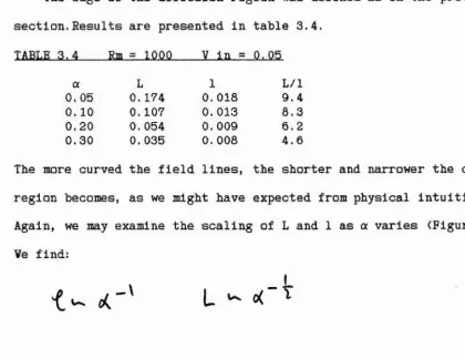
affected by the curvature of incoming magnetic field. Scaling laws for the dimensions of the diffusion region are derived, and the existence of several reconnection regimes Is shown.

Using the same computer code we also simulate tearing modes in

Cartesian geometry under different boundary conditions. By imposing a

suitable perturbation a magnetic island is generated. The plasma flows

show marked differences for the different boundary conditions

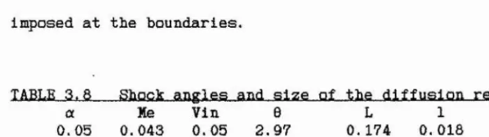
implemented.

Lastly, we examine some aspects of the coalescence instability. The

usual flux function taken to represent a tearing mode island in the

linear growth phase is shown to be erroneous, and we derive a correct

expression. We show that under certain conditions there exists a

ACKKOVLEDOBKB m S

It is a great pleasure to be able to thank Professor Eric Priest for

his supervision of my research studentship over the last three years at

St Andrews, Dr Alan Sykes and the staff of the Theory Division at Culhara

Laboratory for help and guidance, Dr Alan Hood for his supervision of

Chapter 5, Dr Alastair Robertson for much discussion and advice on

numerical simulation, Culham Laboratory for a generous allocation of computer time, colleagues at St Andrews, and friends and family for

their unflagging support and encouragement,

DECLARATION

I, Andrew Mark Colin, declare that the following thesis is a record

of research work carried out by me, that the thesis is ray own

composition, and that it has not been submitted in any previous

application for a higher degree.

Signature of Candidat

Date

Ù

CERTIFICATE

I certify that Andrew Mark Colin has satisfied the conditions of the

Ordinance and Regulations and is thus qualified to submit the

accompanying application for the degree of Doctor of Philosophy.

Signature of Supervisor ....

mSlGRADUAÎE CAREER

I was admitted into the University of St Andrews as a research

student under Ordinance General No. 12 in October 1983 and as a

candidate for the degree of Ph.D. in October, 1984, to work on aspects

of Magnetic Reconnection under the supervision of Professor E.R. Priest.

CONTENTS Chapter 1 Introduction

1.1 Introduction to magnetic reconnection 1.2 Outline of thesis

1.3 The MHD equations

1.4 Analytical models of reconnection 1.5 Previous numerical work

Chapter 2 Numerical solution of the MHD equations 2.1 The MHD equations in conservative form 2.2 Computer simulation

2.3 The SHASTA algorithm

2.4 Solution of the diffusion equation 2.5 Spatial differencing

2.6 Temporal differencing

Chapter 3 Driven magnetic reconnection simulation 3.1 Introduction

3.2 Numerical implementation

3.2.1 Vector potential conversion routines 3.2.2 Compatability relations

3.2.3 Program development 3.3 A typical run

3.4 Effect of varying the magnetic Reynolds number 3.4.1 Size of the diffusion region

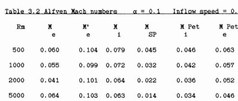
3.4.2 Alfven Mach numbers 3.4.3 Variation of shock angle 3.5 Variation of field line curvature

3.5.1 Size of the diffusion region 3.5.2 Alfven Mach numbers

3.5.3 Variation of shock angle 3.6 Variation of inflow speed

Chapter 4 Tearing mode simulation 4.1 Introduction

4.2 Numerical implementation of the symmetric tearing mode 4.3 Numerical implementation of the open-ended tearing problem 4.4 Experimental results

4.5 Conclusions

Chapter 5 Island coalescence 5.1 Introduction

5.2 Derivation of the energy integral 5.3 Minimisation of the energy integral

5.4 Perturbation expansion of the Euler-Lagrange equation 5.5 Magnetic field due to a tearing mode

5.6 Boundary conditions

5.7 Ideal stability of a current sheet 5.8 First order stability

5.9 Second order stability 5.10 Conclusions

Chapter 6 Conclusions and suggestions for further work

Appendix A Derivation of compatability relations for the two- dimensional ideal magnetohydrodynamical equations

Appendix B Listing of the computer code SHASTA

1. 1

-CHAPTER 1

INTRODUCTION

LJL iJitr.oduct l Qn to . magnet ic ,ra.aQQ.nec1ilQn,

Magnetic reconnection is a phenomenon of fundamental importance in

astrophysical and laboratory plasmas. A magnetic field occupying the

same spatial region as a perfectly conducting plasma or fluid is tied to

the fluid and convected along with the fluid motions, so the initial

topology is preserved in time. However, the introduction of even a small

amount of resistivity allows oppositely oriented magnetic field lines to

come together at current sheets (where a component of magnetic field changes sign) and break, or reconnect, into a different configuration.

Although the width of such current sheets may be very small compared with the scale length of the plasma, this localised effect alters the

global topology of the field. Magnetic reconnection may therefore act as

a decoupling mechanism; a topological constraint on the plasma is removed and new, lower energy states are accessible.

This has two major effects on the plasma. Firstly, new field topologies may be created, which allow transport of plasma ions and

impurities into previously inaccessible regions. Secondly, magnetic

energy within the magnetic field may be released and converted into kinetic and heat energy. Both phenomena are of considerable interest to

astrophysicists and laboratory plasma physicists.

1. 2

-(I) In a solar flare^ reconnection is believed to be the only mechanism

that can give rise to the observed release of very large amounts of

energy (up to 10'-^ J) over the observed short time-scales ( ^ lO'-^ s). In a two-ribbon flare, a magnetic arcade passes through a series of

magnetohydrostatic equilibria, until some critical shear in the field is

reached. The system then becomes unstable, begins to reconnect and

erupts outwards into the corona to produce loops and Hoc ribbons,

together with a wide range of electromagnetic radiation, an

interplanetary blast wave, relativistic and nonrelativistic nuclei, and

high-energy electrons.

(II) Magnetic reconnection is involved in the interaction of the Earth’s

magnetosphere and the solar wind. A current sheet is formed when the

interplanetary magnetic field meets the Earth’s magnetic field. The field lines then reconnect across the sheet, allowing protons and helium

ions from the solar wind to enter the dayside magnetosphere. Evidence

for reconnection has been provided by the ISEE spacecraft in the form of

both quasi-steady processes and flux transfer events (Bagenal, 1985).

Similar phenomena have been observed in the Jovian magnetosphere by the Voyager 1 and 2 spacecraft (Nishida, 1984)

(ill) Magnetic reconnection is an important cause of disruptions in tokamaks and activity in reverse field pinches. Temperatures of around

one hundred million degrees Kelvin are required for the successful

attainment of the Lawson criterion, which relates the number density and

confinement time for a plasma of deuterium nuclei to reach the conditions under which a fusion reaction may occur. To achieve such

conditions in the laboratory requires that the plasma be magnetically

1. 3

-vessel and strong axial magnetic field the torus may be made stable to ideal instabilities. However, there still remain the resistive

Instabilities (such as the tearing mode) which can degrade the

confinement properties of the plasma, enhance anomalous transport of

impurities, and even cause major disruptions that damage the containment vessel.

Despite the fundamental Importance of reconnection theory, it is

still incompletely understood. The subject has traditionally been

divided into the two schools of spoDtaneous and driven reconnection,

with each having its own (largely independent) literature.

Perhaps the best-known spontaneously reconnecting

magnetohydrodynamical phenomenon is the tearing mode instability, in

which the initially anti-parallel field lines about a current sheet 'tear' and reconnect to form a chain of magnetic islands. This process is highly time-dependent (Furth, Killeen and Rosenbluth, 1963). By

contrast, theories of driven reconnection have tended to concentrate on

steady-state solutions to the MHD equations, rather than on time- dependent phenomena. Thus results from the two schools have not been directly applicable, even though the same equations and physical

assumptions are usually used.

It has only been over the last decade, mostly through the medium of

large-scale computer simulation, that any further progress has been made

in the understanding of reconnection theory, and one of the most

striking results is how closely these two schools are now related. For

instance, consider the coalescence instability, in which an ideal

instability forces together two or more magnetic islands, possibly in a

1. 4

-mixture of ideal and resistive MHD effects. Although this instability

occurs spontaneously, the rate at which the islands coalesce will be determined by the maximum rate at which their field lines can reconnect

and is thus determined by the dynamics of driven reconnection. Indeed, we may regard any spontaneously reconnecting system as an ideal system

with the dynamics being locally controlled by driven systems, or a

driven system as a small cross-section of a spontaneously reconnecting

system. A more fruitful approach to use than^this rather arbitrary

division is to assume a set of equations that model the desired physical

system and to vary the boundary and initial conditions under which they

are solved. The bulk of the research presented below forms such a study.

Qu..t H a.a.„Q.f t h&s i s

The remainder of Chapter 1 reviews the current state of analytical

reconnection theory and describes the most important work published to date on numerical reconnection simulations. In Chapter 2 we describe the

fundamental algorithms employed in the computer code SHASTA, together

with their implementation, and give a brief account of recent research on the possiblities and limitations of numerical simulation. Chapter 3

shows how we adapted the code to simulate two-dimensional driven

reconnection, and found a series of steady states when the inflow field

line curvature, magnetic Reynolds number and Inflow speed were varied.

The results are compared with the recent study by Biskamp (1986) and

scaling laws for the reconnection rate and dimensions of the Internal region were deduced to be compared with analytical theory. Chapter 4 is

an account of how the same code was used to model tearing modes with two

1. 5

-the two cases and studied -the reconnection rate as functions of time.

Chapter 5 has an analytical study of the ideal coalescence instability

for a magnetic configuration generated by tearing mode instability, as the field profile due to Finn and Kaw (1977) used in all previous studies is shown to be unrealistic. Chapter 6 concludes with a summary

of the major results and some suggestions for further work.

I

4

3

■4

JL-2 equations,

Throughout the next three chapters of this thesis we shall be

studying solutions to the full non-linear, compressible, resistive, two-

dimensional magnetohydrodynamical equations:

^

C p v ) . o

a t

i

f

(1.3.1)

Induction

(1.3.2)

Mass

continuity

(1.3.3)

Momentum

(1.3. 4)

Energy

I

where

1. 6

-together with an Ohm's law

^ j - %

4

- Ÿ ^ %

" (1.3.6)

and Maxwell's equation

\ ) V H O (1.3.7)

These are supplemented by the equation of state for an ideal gas

(1.3. 8)

where the quantities £, z, p, p, X, t, E, T are non-dimensionalised as follows:

p ^ p 7 p°' - ' 7 " '

P = f Ô = i \ ) j -, ___

lo po) 1

V p X o y / p , ~ I Lo' G ' t

■ rv ( ■T' / / / I - II po T / p

where E', , p', p', X', X', t' ,E', T* are the dimensional magnetic

field, flow velocity, mass density, pressure, current density, spatial

coordinate, time, electric field and temperature, respectively. Eo‘ and

po' are the values of the magnetic field and plasma density in the

1. 7

region, and L.-.,' Is the size of the computational domain. V Is the ratio

of specific heats (= 5/3), R is the gas constant, is the free space

magnetic permeability and is the dimensionless magnetic resistivity.

t

is related to the dimensional magnetic resistivity V\^ , by

(1.3.8)

which is the inverse of the Lundquist number, more commonly referred to

as the magnetic Reynolds number. Ve adopt this usage throughout the rest

of the thesis.

The reader should note that the standard MHD approximations have

been made when combining the Euler fluid equations and Maxwell's

equations of electromagnetism to derive the magnetohydrodynamical equations:

3 D

(i) The displacement current is negligible compared to the

conduction current i.

(11) The plasma is electrically neutral, so that where p^ and Pg_ are the densities of neutral and charged ions within the plasma. For a fuller account of the approximations see, for instance,

Priest (1982, p 92). Note also that our form of Ohm's law is very simple

compared to the more generally used expression

E 4- V. ^ ^ <1.3.9)

(Chen, 1974, p 164) where e is the charge on the electron, n is the number density of charged particles and p^ is the electron pressure. In

1. 8

-1,

â

A.]qalyX.lgAl._..mo.dgls ■ of reconnect 1 on

In this section we give an overview of the most important analytical

MHD reconnection models. We follow the historical development of the subject by considering (in order) the Sweet-Parker, Petschek and Priest- Forbes models.

Sweet (1958) and Parker (1963) considered a two-dimensional, steady-

state system with antiparallel inflow magnetic fields on either side of a neutral line (Figure 1.1). They argue that in a steady state the speed

V* at which plasma carries magnetic field into a sheet of thickness

is just the speed at which the magnetic field diffuses through

the plasma:

/<

V ; ,

where is the magnetic resistivity. For an incompressible medium the

current sheet accelerates the outgoing plasma to the Alfven speed

(1.4.2)

so we may use mass conservation to equate the inflow and outflow mass fluxes:

L v ; , t v , _(1.4.3)

where L is the length of the sheet. This assumes that the current sheet

retains a width over the length of the sheet L, and that L is in fact

- 1. 9 ~

Eliminating between <1.4.1) and (1.4.3) gives the Alfven Mach number

(1.4,4)

from which we may derive the rate at which field lines can be carried

into the system. For a steady state this represents a measure of the

reconnection rate. Ve find

where the magnetic Reynolds number is

LoV-u

(1.4.5)

(1.4.6)

The difficulty with this model is that energy is released from the

magnetic field at rates which are far too slow to account for flare observations. Taking a magnetic Reynolds number of = 10® to 10 ^ a n Alfven speed of a: lOO km/s and a scale length of 10*m gives a

timescale for energy release of tens of days, which is clearly

inadequate when compared to the observed timescales of several tens of minutes. To give more accurate results a very much smaller length scale

must be taken, which is equivalent to making the inflow speed comparable

to the ambient Alfven speed.

The difficulty of reconection rates which are far too small was surmounted by Petschek (1964) in a classic paper based on an idea which

-- 1. -

10-may bifurcate into two pairs of slow magnetohydrodynamical shock waves

which propagate from a central current sheet. The essential difference

between this model and that of Sweet and Parker is that the central diffusion region may be very small, thus decreasing Em and allowing much

higher inflow speeds. The shock waves stand in the flow and (in the

compressible case) convert magnetic energy to the thermal and kinetic energy of two hot jets, which are accelerated from the diffusion region

to reach the local Alfven speed (Figure 1.2).

Soward and Priest (1977) have derived an expression for the

reconnection rate by finding incompressible, two-dimensional solutions

to the MHD equations which are asymptotic and hence valid at large distances from the diffusion region. For large Em they find a maximum

reconnection rate of

.

_

" K-Ir- (1.4.7)

(where ULs, is the external Mach number) which in practice lies between

0.01 and 0.1 and is very much greater than the Sweet-Parker value. Sonnerup (1970) has proposed a model which, while not directly

physically applicable, nevertheless has features in common with several

numerical simulations. He proposes a model with four slow mode expansion

waves which are generated at corners in the inflow. The model predicts that for this configuration the Mach number in the inflow region may

takes values up to unity.

Vasyliunas (1975) has performed a detailed mathematical analysis of the Petschek and Sonnerup mechanisms. As well as putting the Petschek

ro

N

1. 11

-streamlines for a Petschek solution converge on approaching the

diffusion region, an effect caused by a lessened pressure along a line

from the diffusion region outwards. Noting also that the magnetic field

decreases on approaching the current sheet, the solution is an example

of a fast mode expansion. For the Sonnerup solution the streamlines

diverge and the magnetic field increases on approaching the current sheet, thus forming a slow mode expansion.

Priest and Forbes <1986) have presented a new series of analytical solutions that include the Petschek solution and a Sonnerup-like

solution as special cases. They take a finite two-dimensional region

(Ix! <1, tyl < 1) and linearise about a uniform horizontal field in

the upper part of the region ( y 2 0) by setting

E = B. & +

+ . . .

(1.4.8)

1 = Viv 5L + 3b: + ... (1.4.9)

where Viy = V.., and where the lower half of the box consists of

field lines oppositely oriented from those in the upper half. The

boundary conditions for the solution in the upper half are:

Bix = 0 on y = 1

= 0 on the sides (Ixl = 1) Biy = f(x) on y = 0

where f(x) is a function that gives the appropriate normal magnetic

field generated by the slow mode shock waves. The solution is oc>

“L - c^s I d . 4 . i o >

- 1. 12

H e ’"

B;

where B», Bi, M*», Mi are the external and internal magnetic fields, external and internal Mach numbers, respectively. Equation (4) of the

3 <1.4.11)

Ia '>o

where m = n + % and

L ( . B N

" ( L / U l t ^ ^ T n - 6 « 5 U C K t r l

The parameter b categorises the different types of solutions, b = 0

gives a Petschek solution; b = 1 gives a Sonnerup-type solution. When b < 0 we have a family of slow-mode compressions with strongly convergent

flows, while with b > 1 there exists a flux pile-up regime of slow-mode

expansions, with strongly divergent flow and an Increase in magnetic

field on approaching the current sheet. A hybrid regime exists when 0 < |

b < 1, for which there is a fast-mode expansion on the y-axls and a g

slow-mode expansion on the line 1x1 =1. Work is currently in progress

(Robertson and Priest, 1987) to provide a numerical counterpart to these

solutions. a

It is of interest to derive some estimates for the inner (at the Æ

-:W current sheet) and external (at the entrance to the inflow region)

Alfven Mach numbers. For reference the results from the Sweet-Parker and

Petschek theories are grouped together in table 1.1. j

From equation (44) of Priest and Forbes (1986) we have I

- 1.

13-same paper relates the internal, external and normal magnetic field at

the neutral line:

= B e - I

)

Since

i

-<1.4.15)

we may combine these results and substitute back into (1.4.13) to find the internal Mach number for the Petschek model in terms of the external

Mach number.

lable. ,1.1___ Internal.and, external Alfven Mach numbers

Sweet-Parker reconnection:

J

-M«» —

Mi

Petschek reconnection:

- 1. 14 - î

î'

These results will be required in Chapter 3 so that we may compare

results from the numerical work and the analytical theory.

Pxe.YloüS. nu.inericaL.,MO.r.k

This section presents a brief overview of previously published work

on numerical reconnection experiments that are similar to our work.

The first work on numerical reconnnection was performed by Fukao and

Tsuda (1973) who solved the incompressible time-dependent equations of

motion and induction over a rectangular region with boundary conditions imposed so as to give stagnation-point flow. Using a Friedrichs-Lax

scheme and an effective magnetic Reynolds number of 50-500, they

produced a non-zero component of magnetic field perpendicular to the

initial configuration, thus demonstrating that reconnection was

occurring. The experiment had the limitations of insufficient resolution

to resolve the diffusion region, and of not being run for long enough to allow a steady state to develop.

Ugai and Tsuda (1977) study a similar configuration, using a two-

step Lax-Vendroff scheme to solve the compressible MHD equations with an energy equation including ohmic heating; an artificial viscosity is

imposed to ensure stability of the numerical scheme. They take an

initial configuration of a one-dimensional current sheet and assume that Rm ( = 1000 in the external region) is diminished by a factor of 100

within a circle of given radius about the origin. This generates an x-

point in the magnetic field at the origin and produces Fetschek-type

flows, with a plasma jet directed along the x-axis. An integration over

the box shows that the magnetic energy in the box decreases over the

- 1.

15-reconnection mechanism is providing conversion into thermal and kinetic

energy. The same authors (Tsuda and Ugai 1977, Ugai and Tsuda 1979a,b)

have presented further runs of the same experiment, in which they show that holding the electric field vB constant on the inflow boundary gives

evolution to a steady state. The effect of increasing the plasma

resistivity is to shrink the diffusion region and to change the

reconnection rate, which is found to be in agreement with. Soward and Priest's 1977 result.

Ugai (1981 , 1982, 1983) continues this work by considering the effect of different boundary conditions. He finds that replacing the

free inflow boundary by a rigid wall over which there is no mass or

field flux only changes the reconnection rate slightly, but that replacing the exit boundary by the same type of wall inhibits fast

reconnection. Instead, an o-point forms where previously an x-point had been observed.

Hayashi and Sato (1978) solve a similar set of equations but obtain

driven reconnection by imposing the flow speed on their inflow boundary,

rather than letting it free float. They assume zero magnetic resistivity

(ideal MHD) everywhere except where the current density exceeds a critical value to model an anomalous diffusivity, With strongly curved incoming field lines and a free-floating exit boundary they state that a

steady state is reached after 15-20 Alfven transit times, although their

graphs of electric field at the x-point (a measure of the reconnection

rate) do not confirm this. A Petschek-type flow is found, together with an associated bifurcation of the initial current sheet into two standing

1. 16

-boundary replaced by a rigid wall) shows that an island forms within the box, and that an O-point rather than an X-point forms at the origin.

Biskamp (1935, 1986) presents some interesting solutions to the

incompressible equations at high resolution and magnetic Reynolds

number, for which he also has a driven inflow and free floating exit boundary. Despite the appearance of Petschek-type flows and an

associated current-sheet bifurcation, he interprets his results as being nearer a flux pile-up regime. The appearance of a reversed current

region at the downstream end of his diffusion region suggests that a reconection regime of the type considered by Syrovatsky (1971) is taking

place. Because of the importance of these simulations and their

relevance to the study presented in this thesis, a fuller discussion is postponed to Chapter 3 where the results from the two sets of

experiments are compared.

1.6 Reconnection regimes

Ve may summarise and extend Section 1.4 in a classification of six

distinct reconnection regimes for an electrically conducting plasma,

identified by inflow speed V«,, and proposed by Priest (1985):

(I) Very slow reconnection occurs when a system passes through a series of quasi-potential states. For this to occur, the inflow speed V» must

be less than the global diffusion speed , where V«. is the global

ambient length scale.

(II) Slow reconnection, or the Sweet-Parker regime (1958, 1963) occurs when

/VL ... . V.L

Vz.

- I

-

1.17-where Va. j is the Sweet-Parker reconnection rate and Rm is the

ambient magnetic Reynolds number. The diffusion region (or current

sheet) has length Le and the magnetic energy is converted equally into heat and kinetic energy.

(III) Petschek-Sonnerup reconnection develops when

- \ V<. <. V

where scales as 1/log(R^), a result first given by Petschek (1964).

He suggests that a current sheet may bifurcate into four slow mode MHD

shock waves propagating from a central region where the Sweet-Parker

regime is dominant. Since the dimensions of this central current sheet will be much less than the global length scale, the magnetic Reynolds

number governing the reconnection rate within the sheet will accordingly be lower and so the global reconnection rate will be much higher. In

fact, this internal Rm may become of order one and so account for very

rapid reconnection, which has made this model attractive to theorists.

(IV) Unsteady flux pile-up reconnection occurs when

< V.

so that a steady state cannot occur. This regime postulates the

existence of a maximum reconnection rate; magnetic field is brought into the system faster than it can be reconnected and so the flux accumulates

at the diffusion region, causing it to lengthen into a long current

-

1.18-save that the magnetic field strength will increase rather than decrease

on approaching the current sheet.

(V) Impulsive bursty reconnection may be induced after flux pile-up occurs. The central current sheet develops to such a length that it

becomes unstable to the tearing mode instability, leading to the

formation of chains of magnetic islands. These may be expelled from the box in the plasma jet at the end of the current sheet, or coalesce together to form larger islands. Sakai (1983) identifies signatures in

X-ray emission from coronal loops as a manifestation of this instability.

(VI) Turbulent reconnection may develop from the previous regime at

sufficiently high magnetic Reynolds number, with current filamentation

developing on progressivly lower length scales. However, the

difficulties of modelling such a process analytically or computationally

- 2. 1 -

CHAPTER 2

NUMERICAL SOLUTION OF THE MAGNETOHYDRODYNAMICAL EQUATIONS

2l1

The „M P. .équations.

Throughout the next three chapters of this thesis we shall be

studying solutions to the full non-linear, compressible, resistive, two-

dimensional magnetohydrodynamical equations given in Chapter 1 <1.3.1

-1.3.4). To produce a numerical solution we must expand these equations

out into components and cast them into the form of a generalised continuity equation:

where f is the transported quantity and S is a source terra. Ve have

<2.1.2)

<2.1.3)

2. 2

-b u a t b i

^

" h'^

%

3 £ t

3 x a t

(2.1.5)

(2 .1.6 )

(2. 1.7)

EMàSîà solves the MHD equations by splitting them into advective and

diffusive parts. This may be illustrated by examination of equation (2.1.1). Firstly, we solve the advective (hyperbolic) part of the equations, by setting the source term equal to zero;

^ + ^ ' ( P y ] - 0

o t (2. 1.8)

Secondly, we use the transported value f* determined from the first part as initial conditions for the diffusive (parabolic) part of the

equations. Ve set the divergence term equal to zero:

(2.1.9)

The rest of this chapter is a description of some of the numerical

methods used in our computer program that solves the above equations in

two-dimensional Cartesian geometry. The program (or code) is referred to

as SHASTA, after the particular flux-corrected transport algorithm used in the advective subroutines, For a fuller description the reader is

referred to the original papers by Boris and Book (1973, 1976), Weber's

2. 3

-"4

S

Computer simulation,

Traditionally, the three methodologies of astronomy and astrophysics

have been theory, experiment and observation. With the advent of widely f distributed, powerful computer facilities over the last decade a fourth

is now coming into widespread use; that of large-scale numerical

simulation.

Computing the behaviour of a physical system by specifying the governing laws and advancing them in time is a technique that lies

midway between the areas of the applied mathematician and the

experimentalist. In most cases the performance of a calculation on a

computer closely resembles the performance of a physical experiment, in

that the analyst runs an experiment without necessarily knowing what the

results will be. However, the results of a numerical experiment can be

much easier to compare with analytical work than with corresponding observations in the laboratory or above the atmosphere. In a

computational experiment the analyst has complete control over his nodel

universe. He may completely specify the initial configuration and

internal parameters; his experimental probes do not disturb the

experiment; he can study a purely two-dimensional configuration. He Is

also able to try what neither the theoretician nor the experimentalist

may, by testing the sensitivity of phenomena to independent theoretical

approximations (Arnett, 1985).

Most serious work in numerical simulation has come to require the power of supercomputers, such as those built by Cray Research, which

~ 2.

-next decade a number of machines with non-Neumann architectures

(Pearson, Richardson and Toussaint, 1985) will be specially built to treat problems of comparable complexity and processing cost to those

examined in the subsequent chapters. These computers will be based on

large arrays of microprocessors configured in a two- or three-

dimensional matrix so that one processor is available for every

gridpoint at which the governing equations are to be solved. It may be

that such machines will eventually become more powerful for application to this class of problem than non-dedicated supercomputers, where

constraints such as the time taken for an electrical signal to cross the computer at the speed of light will put a limit on the ultimate speed of operation.

The program that produced the results presented in Chapters 3 and 4

was developed on the two DEC VAX 11/785 machines at St Andrews, and was

run both at St Andrews and on the UKAEA's PRIME at Culham Laboratory,

Oxfordshire, as a 'front-end' machine for the Harwell CRAY-1.

I hQ SHASTA...aiIg.Qr.i.thffl

In this section we give a brief account of SHASTA, one of a class of

flux-corrected transport (FCT) algorithms first presented by Boris

(1973). These schemes are designed to perform accurate transport of

discontinuities in fluid dynamical simulations, and hence the use of

such an algorithm will be particularly helpful when we come to simulate MHD shocks in the Petschek model.

Conceptually, such an algorithm consists of two stages: a transport

or convective stage, followed by an anti-diffusive or corrective stage.

2. 5

-of actual mass and energy densities, so steep gradients and inviscid

shocks are handled much more accurately than by a conventional second-

order scheme such as the Lax-Vendroff (Roache, 1976).

As an illustration of the method we here give a simple geometrical interpretation of FCT applied to the one-dimensional continuity equation

jÿ

0 ^ ^ ^ f ' (2.3.1) Vi

The method may easily be extended to multi-dimensional applications.

4

beginning of an iteration ( t = 0 ). Ve assume that the densities are known and that the velocities 1 V/J are known at t = (St/2, half a

timestep ahead. Ve require the densities ^ ^ ^ at the end of the

timestep when t = (St.

The method begins by considering a typical fluid-element trapezoid,

formed by connecting adjacent densities with straight line segments. The

density profile thus constructed is consistent with the definition of

the total mass

h

On Figure 2.2(b) we have sketched short arrows, showing how these fluid

elements and their boundaries might convect in a Lagrangian sense. To

ensure positivity, Boris restricts his analysis to I v #t/#x I < %

where v = max (IVjl ) so that no fluid element boundary convects past a

Stage I ;

... transport

o

j-fl

Figure 2.1 Converted fluid trapezoid

y

p

A t

0+1

2 . 1 (c)

p

to ) b \\ , is

(2.3.5)

- 2. 6 - 4

g

cell boundary. In our full code we take a more restrictive condition %

that enables us to treat MHD waves; this Courant-Friedrichs-Lewy (or I CFL) condition is described below.

We follow the motion of the fluid element for one timestep in a 4 fN Lagrangian sense. The complete transport prescription, relating | )

P 0^ ' t t I ( Pi-H - P<) ) (2.3.3) I

+ ( 9 - ) p j

where for greater accuracy the j ^ derived from linear

interpolation back on the grid may be used (Figure 2.2(c)). These are given by

I

- C l - / i ] v i + ( c j / l )

,

I

^ -12 I /z) (2.3.6)

C V •'< 0 )

where C

j

|

S

/ I .

For a uniform velocity field this reduces to the simpler form

P j - Pi - l(pj+'"pj''/ +

~ 2. 7

-This formula is a simple two-sided differencing of the convection term,

plus a strong zero-order diffusion. Without this velocity-independent diffusion we just have the result found by using the two-step Lax-

Wendroff algorithm (Mitchell, 1969; Roache, 1976), with the usual

second-order dispersion and velocity-dependent diffusion.

The strong diffusion corresponds to acting on the initial density profile ^ pj ^ in the following way;

(2.3.8)

For the zero-velocity case the diffusion coefficient is strictly 0.125.

In the case of nonzero velocities 4 ^ is 0.125 plus small wave-number

and wave-number dependent terms. A von Neumann analysis of this equation

shows that the amplification factor is always less than unity for ^ < 0.5, so the transport scheme is always stable.

S-tage II: Anti diffusive transport

It is straightforward to remove the zero-order diffusion from stage I by applying an equal and opposite anti-diffusion. Since the previous

Ù i

readily be inverted by the use of standard algorithms. However, the equation represents an implicit tridiagonal system for ^ ^ ^ ^ it may

fastest and simplest way to remove this residual diffusion is by an explicit anti-diffusion equation

“ 2. 8 ”

This equation has the disadvantage of not conserving positivity.

Consider the example shown in Figure 2.2 . The antidiffusion imposed in

stage II, which is only intended to remove numerical errors introduced

in stage I, in fact brings in new numerical errors at the labelled grid points. New maxima and minima are formed where they are physically

unreasonable, and the new minimum is negative. We cure these features by invoking the principle of flux corrected transport.

Stage.. IlI.L_.Elux £orr.e£.tl-O.Q,

To remove the nonpositivity it is more direct to work with the mass

fluxes directly. We may rewrite the antidiffusion formula

T \ _ I

where the antidiffusive mass fluxes are defined as

<2.3.10)

(2.3.11)

This rewritten antidiffusion formula has two important properties: i) The antidiffusive fluxes and j! describe explicit

transfers of material.

ii) The equation is strictly conservative, no matter what values the

fluxes take, as every flux is added once and subtracted once somewhere else (except at the boundaries).

We are thus led to the principle of flux-corrected transport:

a#

P

t?; O

- 2. 9 ~

The antidlffusion stage should generate no new maxima or minima in the 4 '4

solution, nor should it accentuate already existing extrema. a

■ i

at any grid point beyond the density value at neighbouring points. This is the origin of the name 'flux-corrected transport' and is the crux of

12)

where

This scheme clearly maintains positivity. To make the limitation

quantitative without violating conservation, we correct the 4

antidiffusive mass fluxes. The are limited term by term so 4 that no antidiffusive-flux transfer of mass can push the density value 4

I

JÏ

the method. J'

The corrected fluxes ^ are given by the formula :%

*

% P j — P 3 (2.3.13) I

and the fluxes ^ are replaced in the original antidiffusion

equation. The quotation marks about the factor 0.125 indicate that a | ‘I more exact cancellation of factors can be achieved if even rough

approximations to the velocity and wavenumber dependent corrections are

included.

An application of this schema to sharp gradients gives rise to the

- 2.

10-that the Ranklne-Hugoniot relations (Jeffrey and Taniuti, 1964) are still satisfied.

of which the best known is the Alternating-Direction Implicit (ADI)

(Mitchell, 1969). The scheme we choose here is also implicit and has the

advantage, as do all this class of algorithms, of being unconditionally stable so that a timestep of any size may be taken without loss of

showing that ^ & j j may be found by solving the matrix equation

(ignoring the boundary conditions)

? I

I

2

Solution of the diffusion. eq.uat.i,o.a.

I

There exist several ways to solve the two-dimensional diffusion

equation

J

numerical stability. Differencing the x-component of (2.4.1) gives

,

a-:;

n -;

A t '

This expression is first order in time and second order in space.

Rewriting (2.4.2),

2. 11

-o

o

... O 1

L

l u

Av

&K, <2.4.4)

This may be easily solved on noting that the matrix is tridiagonal. There exist several explicit, non-iterative algorithms to invert such

matrices; we choose that of Crout (Burden et ai, 1981).

For a numerical scheme of this type the boundary conditions must be imposed implicitly on the form of the matrix, unlike the advective part

of the code where they must be imposed explicitly. For instance,

consider the case of a zero first-order derivative boundary condition.

Denote the entry in the ith row and jth column by a(i,j); then the

matrix may be represented in the form [a(i,J)3. To impose a zero normal

A ft

derivative at the upper boundary, let % , ~ ^ ° * T^be matrix and vectors of magnetic field will then assume the form

^ 11 O » • • ! “ a , ' ₁ h , \ — <^1.1 Ô • • • !■; o

1 °

O * - _(ÎÎ 1

i

1

Bv, i = _{j Bs!}i

I ^

(2.4.5)

2. 12

-as required.

ut*^!

* (2.5.1)

where nz is the number of points along the z-axis < = 60) and f is the fractional increase in spacing from one grid-point to the next ( =

0.10). The lowest grid spacing is thus Az - 0.012 and the highest is Az 0.133. Ve found from experiment that f could not exceed about 0.13 or

the code went unstable.

Ve are limited by the grid resolution as to the maximum magnetic

Reynolds number that may be taken. In the grid separation instability, a cascade of energy proceeds from long wavelengths to short ones due to

the nonlinearity of the MHD equations; the physics 'literally slips

i

where the vectors are the values of magnetic field on a column of the ^ numerical grid, The reader will note that expanding the second row gives

%-Î

2 ^ S.pat.lal..,dif.f.er.e.nc.l.ng.

•y

The computation is performed in Cartesian coordinates over a

rectangular array of 40x60 grid points. The points are uniformly spaced

in the x-direction but are non-uniformly spaced in the z-direction to

ensure higher resolution at one edge of the box. The i'th grid point in

- 2.

13-through the cracks' (Pearson et al, 1985), This need not affect the

behaviour of the code as long as we can be sure that all wavelengths are being modelled accurately.

One way to do this is to use a spectral code, in which the MHD

equations are Fourier analysed in space and the governing equations in

Fourier space are solved numerically. Such a scheme ensures that all length scales can be accurately described throughout the calculation as long as computation is stopped when significant activity appears in the

highest wavenumbers. The difficulty with such a scheme is that the

treatment of boundary conditions becomes complicated for any but the simplest configurations, with one analytical expression required for

each harmonic in both directions. Since hundreds of harmonics are

required for problems of interest, this approach presents some rather

severe difficulties. Matthaeus and Montgomery (1981) have performed a study of the double tearing mode in two dimensions with such a spectral

code, the advantage being that for such a configuration only symmetry

conditions need be imposed on the boundary. They find interesting

evidence of current filamentation, a feature observed in some laboratory

experiments (Stenzel et al, 1986) but not in any finite-difference

calculations performed to date. A spectral approach is also suitable for

a study of homogeneous turbulence.

Ve choose instead to follow the approach of Forbes and Priest (1983), who attempt to model all length scales within a finite-

difference scheme and thus to avoid grid-separation instability. They

argue that the numerical grid spacing should be less than the

Kolmogorov dissipation scale lengths X f

j _{"y 3} < l t v -I

;

- ^

2. 14

-(Landau and Llfschitz, 1959, p 122) where and £.\/ are the total

magnetic and kinetic energies, respectively. In our equations the viscosity arises only from numerical effects and the magnetic

conductivity is the major significant source of diffusion. We therefore

ensure that the grld-resolution is sufficient at the current sheet to cover the shortest wavelengths arising at any time.

Eastwood and Arter (1985) have performed a important and 4I

controversial study of this type of instability in the context of simulations of tokamak disruptions. They perform a detailed analytical

study of aliasing error,a common cause of 'blow-up’ of solutions. As an

Illustration they consider the discretlsed, Fourier transformed fluid 'g

1

equations. Let the shortest wavelength have wavenumber K and let the velocity spectrum be filled for k up to K; then the non-linear advection

terms attempt to generate flows with wavenumbers up to 2K. Those in the

range K + 1 to 2K pretend to be, or 'alias', flows of wavenumber less

than K. If the physical process being modelled is a cascade of energy from large to small scales, a positive feedback instability is possible,

since energy which should have been transferred to small length scales is Instead transferred to long ones. The instability usually manifests

itself first as a violation of energy conservation followed by the

appearance of arbitrarily large velocities and magnetic fields so that

•I the timestep (here determined by the CFL condition) drops towards zero, 4

I

% However, identical behaviour is seen when there is a mathematical or

programming error in the boundary conditions or vector potential

2. 15

-against mistaking non-linear instabilities for effects caused by

programming errors in the context of fluid-dynamical simulations. It seems likely that this instability caused Forbes and Priest's

study of line-tied reconnection to end prematurely. Ve have also

observed the effect in some of our tearing mode simulations, which are

very similar to theirs. Chapter 4 describes how one physically allowable perturbation, imposed to initiate magnetic tearing, drove the code

unstable in a few Alfven times while others let the code run

indefinitely. In the light of these ideas we suggest that the first

perturbation contained harmonics at higher wave-numbers, so that the

cascade process for the first run took much less time to reach the aliasing stage than the second.

Boundary conditions are imposed explicitly by the modules BOÜNDY and

Implicitly from within AFEOMB, BFROMA and DIFUSE. These are listed in Appendix B.

Temporal differencing

The timestep At is determined by the Courant-Friedrichs-Lewy condition (Potter, 1981)

A t 3 A A

where A is the smallest grid spacing in the mesh < = minCAx, Az) ), Vx and Vz are the x and z components of the plasma velocity, and

is the fast mode wave speed. A is the Courant number which is set to 0.2

4 y:

-î

3. 1 - f

CHAPTER 3

DRIVEN MAGNETIC RECONNECTION

Introduction

In this chapter we apply the computer program described in Chapter 2 to a study of steady-state driven magnetic reconnection. Because of the

work performed to date has been numerical CBirn, 1985; Biskamp, 1986;

Forbes and Priest, 1982, 1983, 1984; Lee and Fu, 1986; Matthaeus and

Montgomery, 1981; Sato and Hayashi, 1979; Ugai, 1984; Ugai and Tsuda,

1977). The results, reviewed in Priest (1985) have shown many new and unexpected features, such as the rapid creation and annihilation of

neutral points found by Forbes and Priest (1982 , 1983a, b) and the

emergence of plasma jets from a Y-point at the end of a current sheet in Biskamp's simulation (1986), as described and analysed by Soward and

Priest (1986). However, the effect of varying the boundary conditions and internal parameters remains poorly understood.

Chapter 3 presents the background and results to a series of

numerical experiments in which three externally adjustable parameters are systematically varied and their effect on the solutions examined. In

section 3.2 we describe the numerical implementation of the driven

reconnection problem together with an account of the development of the

code. In section 3.3 a 'standard run' with typical magnetic Reynolds number and boundary conditions is analysed in detail. In sections 3.4,

3.5 and 3.6 we show the effect of varying incoming field line curvature,

non-linearity of the MHD equations and the resulting difficulty in i

<3.2.1)

Suriacfi..2 (symmetry);

^ V t =

V l " V : " V t

3. 2

-plasma resistivity and plasma inflow speed. Sections 3.7 and 3.8 have

some general comments on the dynamics of driven reconnection arising from this study.

Numerical. ImplemeatallQn

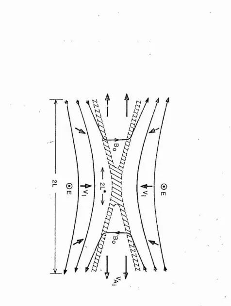
The field topology we choose to study has two symmetrical, adjacent,

two-dimensional antiparallel flux systems with externally imposed flow and field curvature. Such a configuration might occur inside a tokamak

when two islands with different ja, n numbers overlap and coalesce, or in

3

the Earth's geomagnetic tail during a substorm (Figures 3.1, 3.2). We Ig chose to impose symmetry in both the x- and y-directions, which may be

exploited to reduce the number of grid points required, and hence the f| j| computer time needed for each run. Instead of considering the whole

system (Figure 3.3), we may instead examine only one quadrant (Figure i;j 4 3.4). This precludes the occurrence of some asymmetric tearing phenomena j

but will otherwise give exactly the same information. H

For convenience, we assign numbers to label each of the four | '“I numerical boundaries, as shown on figure 3.4. In analytical form the |

boundary conditions are 3

o o

4

Figure 3.1 Coalescence of magnetic islands

.1

u

m

>

Co

G.

f+

«eating) X

figure 3.4

^^ngie

quadrant

system

3, 3

-^ 3 Ù 3 p 3 R x

5 x ' S x ’ 3 x ’ 5 x ’ ° a X " ) t "

Sur face ■4_.Cürlvea inflow);

H X ^ ^ Ÿ ) P imposed (3.2.4)

where the variables and their non-dimensionalisation are defined in

Chapter 2.

To use an analytical expression for a boundary condition, we must find a numerically equivalent condition so that the code will assign

meaningful values to the gridpoints at the edge of the numerical box. For an axis of symmetry this is straightforward; we define the row or

column of points one gridpoint in from the boundary to be the edge of

the system, and calculate the values of all independent variables at the edge on the basis of their values two grid-points in. Specifying the

subscript on a variable as the index along the normal to each surface,

the boundary conditions for edges 1 and 2 are implemented as

Surface 1 (symmetry)

R I » R (3.2.5)

Surface

2

(symmetry)

b I ^ P \

R x x

- o

V

3. 4

-To Impose the values of all variables at the inflow boundary is

similarly straightforward (although the reader should note the risk of

overspecification mentioned in Section 2.3.3 and in Appendix A).

S.urface....4 (driven inflow)

R X ^ ^ R X ‘,w V X I Vx

^ - p

(3.2.7)

The implementation of a free-floating boundary illustrates a

limitation of the finite-difference technique. For an analytical

analysis of an astrophysical plasma a boundary may safely be taken to be

at infinity, but the computational domain must of necessity have a

finite number of gridpoints. One way to overcome this is to

isomorphically map the finite computational domain onto an infinite region, as did Weber (1978). However, the resolution becomes

correspondingly poor towards infinity so that an MHD wave propagating

into this region will eventually trigger a numerical instability

(Forbes, 1987). Alternatively, a Sommerfeld radiation condition

O C

may be used, where f is a flow variable and Vf- is the magnitude of the

local phase speed of the wave quantity (Orlanski, 1976; Han et al,

1983). Forbes (1987) observes that this condition forces the wave at the boundary to be outward propagating, giving a well-posed initial-

boundary-value problem. Despite this, numerical methods based on the full Sommerfeld condition may be prone to instability (Israeli and

3. 5

-Ve choose instead to implement the much simpler boundary condition

of first-order extrapolation of all variables:

(3.2.9) — = 0

where X k is the coordinate perpendicular to the surface under

consideration. Chu and Sereney (1974) have performed a comparison of

seven different methods of formulating boundary conditions at an outflow boundary for a one-dimensional hydrodynamical open-boundary problem. They found that only first-order extrapolation and a method based on

extrapolation of the characteristics (equivalent to the Sommerfeld condition) gave results consistent with the known analytical solution. The other, more complex methods gave less accurate results. Hence we

believe that this method is one of the best for the problem.

Given time, we would have improved these boundary conditions by

using the very similar method described by Caraerlengo and 0'Brien{^%**):

4 X ' - i l

<3.2.10)

>3 If the local wave is incoming, it does not change over an iteration, s|

while if the local wave is outgoing p is given by first order

j

extrapolation in space and time, approximating a Sommerfeld condition. I Alternatively a simple extrapolation may be combined with a wave-

3. 6

The initial conditions are

Vx — 0

Vz = 0

Bx= sin ( i r z /2 w ) ( z < w )

Bx= 1 ( z > w ) (3.2.11)

Bz = 0

P = 1

p = ( 1 + j3 - 1 ai 1 Bt )/2

where w is the width of the initial current sheet ( = 0.05) and the

ratio of gas to magnetic pressure, is 0.1. The pressure condition

ensures the system is in magnetohydrostatic equilibrium at t = 0.

VaglÆr-...p.at.^&.tlaL...g.QaLVê£slo.R. CQUtlûaa

Ve choose to use the magnetic vector potential A as a supplementary variable. Several advantages arose from this. Only A need be treated in

the the diffusive part of the program, rather than both components of

magnetic field, with a resulting saving in computing costs. Since g, - curl A, elementary vector identities ensure that div B = 0 identically at all times. However, routines to convert from A to B and back at every iteration were still required since the advective equations are cast in

terms of B. Also, more complex boundary conditions that impose A, Bx and Bz selfconsistently were required, and finding

■

The disadvantage is that a large number (at least 10%) of the gridpoints -ç must lie in this region, which is not modelling any physical processes.

3. 7

-workable expressions (especially at the corners of the box) proved to be

extremely difficult.

The calculation of B from A is straightforward. A two point formula is used to obtain the derivative of A in the x direction:

^ A

)

This gives full second order accuracy on the uniformly spaced axis. For

a similar accuracy order to hold in the z-direction a four point formula

would be required (Roache, 1976, p 20). We decided that the associated

complexity of the associated boundary conditions would have been too

expensive in development costs and implemented another two point formula |

(Schnack, 1978): j

B N 2_ N j + t — (\J— '

^ ^ t k + ^ - A . t

where

t t Si ~

t - t j ^

The truncation error is

(3.2.13)

(3.2.14)

A - t A +4: H A - 1

<3.2.15)

so that (3.2.13) is formally first order accurate, becoming second order

<3.2.17)

Z t +

t--T t--T t--T

and thus we have ’effective’ second order accuracy.

To derive A from B proved to be a considerably more complex problem.

To calculate A one of the two first-order differential equations

must be integrated subject to the boundary conditions, and the first difficulty becomes apparent: if the vector potential is integrated up a

column or along a row two boundary conditions for A have to be imposed

on the solution of a first order system, leading to overspecification. The first approach tried for the driven reconnection problem (and

the one eventually adopted) was straightforward integration of the x-

component of magnetic field in the z-direction:

. f (3.2.19)

1

I

- 3. 8 - .1

A

5 V* (3.2.16)

A - 1

where r = 1 t ^ ^ a small constant. In this case (3.2.15) becomes

The coefficient of the first order term behaves like ÿ

3. 9

-The value of the tline-dependent vector potential was specified at the

inflow boundary and at the two rows further in, and the field was

integrated down to the bottom of the box. To maintain second order accuracy B was integrated over alternate pairs of points, an approach

used by Forbes and Priest (1982) . To check for consistency, the two

conversion routines BFROHA and AFROMB were run alternately on the intial magnetic field profile, and to within single precision VAX arithmetic

the results were consistent to 6 decimal places after several hundred

iterations.

With low values of this approach worked well, but decreasing

gave some noise in the field lines, which are here plotted as contours #

of constant A. The difficulty is probably purely numerical, in that the

equations which convert B from A are not being inverted in precisely the

same form. That is, while a three point formula is used to differentiate f

A, a two point formula derives A from B and so ’decoupling* can occur

between the values of A at odd and even rows. This gives rise to the M

noise, which is caused by rapid alternations of A from gridpoint to

gridpoint. This, nonphysical effect is probably not seen when low values

I"

of Rm are taken because the associated high Fourier modes and steep

■I gradients are damped out by the high resistivity. It is possible that % 3.

this is the cause of some of the numerical instabilities seen by Forbes 5

in his work (1982, 1983a, b>, as well as the Kolmogorov length-scale and

I

aliasing instabilities discussed in Chapter 2, section 5.

An obvious further approach would be to modify the vector potential

3 . 1 0

-Althüugh cheap to run, we did not have enough time to write and debug

this extension to the code.

3.,..2.^2 Compat Ibllity r.e.Iat i ohs

The MHD equations we solve in this chapter <2.1.1 - 2.1.4) are of mixed hyperbolic-parabolic character, since the introduction of

dissipation adds second-order terms to the system. With even a partly

hyperbolic system, the need to assign values to each of the variables on

boundaries over which there is a mass and field flux will lead to over­ specification and the consequent formation of a boundary layer. This

section describes a consistent formulation to avoid over-specification

by determining the values of some of the boundary variables from the

system of equations being solved. The method proceeds through

determining the characteristic equations of the system and transforming

them to lie along the projected characteristics as described in Appendix 3

I

A. A subset of the resulting compatability relations may then be solved; :|

the number will depend on how many variables cannot be specified at that 3

point, which in turn equals the number of characteristics leaving the

computational domain ( Courant and Hilbert, 1962, p 473 ). J

4

Hu and Vu (1985) give a full discussion of the characteristics of '

1

the two-dimensional ideal (purely hyperbolic) equations. Here we may . i

consider the simpler case of a one-dimensional scan of the ideal two- j

dimensional equations; ideal, because we assume resistive effects to be i

unimportant everywhere away from the x-point; one-dimensional, because

our numerical scheme scans in the x- or z-direction while ignoring

4- C v t - v s ] B

o r j: <3.2.21)

3.J3.1.3-- grQgraa. .de.yfi.1 opinent

Given the problem as defined in the previous sections, a suitable

combination of initial and boundary conditions had to be found which

allow the system to evolve in time to give asymptotically steady-state reconnection. For development purposes we omitted the use of any

compatability relations, as they invariably complicated the behaviour of

the system to such an extent that it was unclear which effects were

physical and which numerical. For instance, a crude approximation to the compatability relation was obtained by setting

3 . 1 1

-Cartesian geometry the projected characteristics will just lie along the

art boundary, where n is the unit normal to the boundary at the

specified point. Ve restrict further analysis to the z-t plane since the characteristic equations are primarily of interest to us in the context

of the driven inflow boundary (z = 0), and refer the reader to Appendix

A for a full treatment of the problem. For reference, we observe here

that for the inflow regime under consideration < -Vs ( Vin ( 0 ) only -Sj

1

one compatability relation need be solved, which is 'I

(Lx Rt Dt\/x - A

DtVk

<]

+

Bx

Bx

Bx Vx

(3.2.20)

I

4"

D:k p ::<)

|

where

m. ^ <3.2.22)