MRPR: A MapReduce Solution for Prototype
Reduction in Big Data Classification
Isaac Trigueroa,, Daniel Peraltaa, Jaume Bacarditb, Salvador Garc´ıac,
Francisco Herreraa
a
Department of Computer Science and Artificial Intelligence, CITIC-UGR (Research Center on Information and Communications Technology). University of
Granada, 18071 Granada, Spain
b
School of Computing Science, Newcastle University, NE1 7RU, Newcastle, UK
c
Department of Computer Science. University of Ja´en, 23071 Ja´en, Spain
Abstract
In the era of big data, analyzing and extracting knowledge from large-scale data sets is a very interesting and challenging task. The application of stan-dard data mining tools in such data sets is not straightforward. Hence, a new class of scalable mining method that embraces the huge storage and processing capacity of cloud platforms is required. In this work, we propose a novel distributed partitioning methodology for prototype reduction tech-niques in nearest neighbor classification. These methods aim at representing original training data sets as a reduced number of instances. Their main purposes are to speed up the classification process and reduce the storage requirements and sensitivity to noise of the nearest neighbor rule. However, the standard prototype reduction methods cannot cope with very large data sets. To overcome this limitation, we develop a MapReduce-based framework to distribute the functioning of these algorithms through a cluster of comput-ing elements, proposcomput-ing several algorithmic strategies to integrate multiple partial solutions (reduced sets of prototypes) into a single one. The pro-posed model enables prototype reduction algorithms to be applied over big data classification problems without significant accuracy loss. We test the speeding up capabilities of our model with data sets up to 5.7 millions of
Email addresses: [email protected](Isaac Triguero),
instances. The results show that this model is a suitable tool to enhance the performance of the nearest neighbor classifier with big data.
Keywords:
Big data, Mahout, Hadoop, Prototype reduction, Prototype generation, Nearest neighbor classification
1. Introduction
The term of big data is increasingly being used to refer to the challenges and advantages derived from collecting and processing vast amounts of data [1]. Formally, it is defined as the quantity of data that exceeds the pro-cessing capabilities of a given system [2] in terms of time and/or memory consumption. It is attracting much attention in a wide variety of areas such as industry, medicine or financial businesses because they have progressively acquired a lot of raw data. Nowadays, with the availability of cloud platforms [3] they could take some advantages from these massive data sets by extract-ing valuable information. However, the analysis and knowledge extraction process from big data become very difficult tasks for most of the classical and advanced data mining and machine learning tools [4, 5].
Data mining techniques should be adapted to the emerging technologies [6, 7] to overcome their limitations. In this sense, the MapReduce framework [8, 9] in conjunction with its distributed file system [10], originally introduced by Google, offers a simple but robust environment to tackling the process-ing of large data sets over a cluster of machines. This scheme is currently taken into consideration in data mining, rather than other parallelization schemes such as MPI (Message Passing Interface) [11], because of its fault-tolerant mechanism, which is crucial for time-consuming jobs, and because of its simplicity. In the specialized literature, several recent proposals have focused on the parallelization of machine learning tools based on the MapRe-duce approach [12, 13]. For example, some classification techniques such as [14, 15, 16] have been implemented within the MapReduce paradigm. They have shown that the distribution of the data and the processing under a cloud computing infrastructure is very useful for speeding up the knowledge extraction process.
removing noisy and redundant data. From the perspective of the attributes space, the most well-known data reduction processes are feature selection and feature extraction [18]. Taking into consideration the instance space, we highlight instance reduction methods. This latter is usually divided into instance selection [19] and instance generation or abstraction [20]. Advanced models that tackle simultaneously both problems are [21, 22, 23]. As such, these techniques should ease data mining algorithms to address with big data problems, however, these methods are also affected by the increase of the size and complexity of data sets and they are unable to provide a preprocessed data set in a reasonable time.
This work is focused on Prototype Reduction (PR) techniques [20], which are instance reduction methods that aim to improve the classification capa-bilities of the Nearest Neighbor rule (NN) [24]. These techniques may select instances from the original data set, or build new artificial prototypes, to form a resulting set of prototypes that better adjusts the decision bound-aries between classes in NN classification. PR techniques have proved to be very competitive at reducing the computational cost and high storage require-ments of the NN algorithm, and also improving its classification performance [25, 26, 27].
Large-scale data cannot be tackled by standard data reduction techniques because their runtime becomes impractical. Several solutions have been de-veloped to enable data reduction techniques to deal with this problem. For PR, we can find a data-level approach that is based on a distributed parti-tioning model that maintains the class distribution (also called stratification). This splits the original training data into several subsets that are individu-ally addressed. Then, it joins each partial reduced set into a global solution. This approach has been used for instance selection [28, 29] and generation [30] with promising results. However, two main problems appear when we increase the data set size:
• A stratified partitioning process could not be carried out when the size
of the data set is so big that it occupies all the available RAM memory.
• This scheme does not consider that joining each partial solution into
a global one could generate a reduced set with redundant or noisy instances that may damage the classification performance.
To do so, we rely on the success of the MapReduce framework, designing carefully the map and reduce tasks to perform a proper PR process. Con-cretely, the map phase corresponds to the splitting procedure and the appli-cation of the PR technique. The reduce stage performs a filtering or fusion of prototypes to avoid the introduction of harmful prototypes to the resulting preprocessed data set.
We will denote this framework “MapReduce for Prototype Reduction” (MRPR). The idea of splitting the data into several subsets, and processing them separately, fits better with the MapReduce philosophy, than with other parallelization schemes because of two reasons: Firstly, each subset is indi-vidually processed, so that, it does not need data exchange between nodes to proceed [31]. Secondly, the computational cost of each chunk could be so high that a fault-tolerant mechanism is mandatory. For the reduce stage we study three different strategies, of varying computational effort, for the integration of the partial solutions generated by the mappers.
Developing a distributed partitioning scheme based on MapReduce for PR motivates the global purpose of this work, which can be divided into three objectives:
• To enable PR techniques to deal with big data classification problems.
• To analyze and illustrate the scalability of the proposed scheme in terms
of classification accuracy and runtime.
• To study how PR techniques enhance the NN rule when dealing with
big data.
To test the performance of our model, we will conduct experiments on big data sets focusing on an advanced PR technique, called SSMA-SFLSDE, which was recently proposed in [27]. Moreover, some additional experiments with other PR techniques will be also carried out. The experimental study includes an analysis of training and test accuracy, runtime and reduction capabilities of PR techniques under the proposed framework. Several vari-ations of the proposed model will be investigated with different number of mappers and four data sets of up to 5.7 millions instances.
and discuss the empirical results in Section 4. Finally, Section 5 summarizes the conclusions of the paper.
2. Background
In this section we provide some background information about the topics used in this paper. Section 2.1 presents the PR problem and its weaknesses to deal with big data. Section 2.2 introduces the MapReduce paradigm and the implementation used in this work.
2.1. Prototype reduction and big data
This section defines the PR problem, its current trends and the drawbacks of tackling big data with PR techniques. A formal notation of the PR problem
is the following: Let T R be a training data set and T S a test set, they are
formed by a determined number n and t of samples, respectively. Each
sample xp is a tuple (xp1,xp2, ...,xpD, ω), where, xpf is the value of the f-th
feature of the p-th sample. This sample belongs to a class ω, given by xpω,
and a D-dimensional space. For the T R set the class ω is known, while it is
unknown for T S.
The purpose of PR is to provide a reduced set RS which consists of rs,
rs<n, prototypes, which are either selected or generated from the examples
of T R. The prototypes of RS should be calculated to efficiently represent
the distributions of the classes and to discern well when they are used to
classify the training objects. The size of RS should be sufficiently reduced
to deal with the storage and evaluation time problems of the NN classifier. As we stated above, PR is usually divided into those approaches that are limited to select instances fromT R, known as prototype selection, and those that may generate artificial examples (prototype generation). Both strategies have been deeply studied in the literature. Most of the recent proposals are based on evolutionary algorithms to select [32, 33] or generate [25, 26] an
appropriateRS. Furthermore, there is a hybrid approach between prototype
selection and generation in [27]. Recent reviews about these topics are [19] and [20]. More information about PR can be found at the SCI2S thematic
public website on Prototype Reduction in Nearest Neighbor Classification:
Prototype Selection and Prototype Generation 1.
Despite the promising results shown by PR techniques with small and
medium data sets, they lack of scalability to address big T R data sets (from
tens of thousands of instances onwards [29]). The main problems found to deal with large-scale data are:
• Runtime: The complexity of PR models is O((n·D)2
) or higher, where
n is the number of instances and D the number of features. Although
these techniques are only applied once on a T R, if this process takes
too long, its application could become inoperable for real applications.
• Memory consumption: Most of PR methods need to store in the main
memory many partial calculations, intermediate solutions, and/or also the entireT R. WhenT Ris too big, it could easily exceed the available RAM memory.
As we will see in further sections, these weaknesses motivate the use of distributed partitioning procedures, which divide theT Rinto disjoint subsets that can be manage by PR methods [28].
2.2. Mapreduce
MapReduce is a paradigm of parallel programming [8, 9] designed to process or generate large data sets. It allows us to tackle big data sets over a computer cluster regardless the underlying hardware or software. It is characterized by its highly transparency for programmers, which allows to parallelize applications in a easy and comfortable way.
Based on functional programming, this model works in two different steps: the map phase and the reduce phase. Each one has key-value (< k, v >) pairs as input and output. Both phases are defined by a programmer. The map phase takes each < k, v > pair and generates a set of intermediate < k, v >
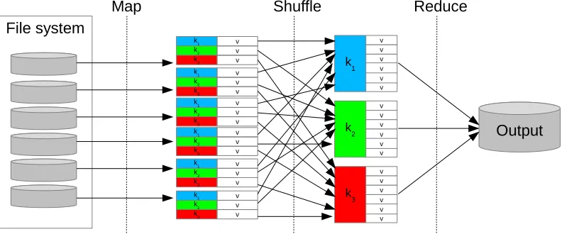
Figure 1: Flowchart of the MapReduce framework
An illustrative example about the way of working of MapReduce could be find the average costs per year from a big list of cost records. Each record may be composed by a variety of values, but it at least includes the year and the cost. The map function extracts from each record the pairs
< year, cost > and transmits them as its output. The shuffle stage groups
the < year, cost >pairs by its corresponding year, creating a list of costs per
year < year, list(cost)>. Finally, the reduce phase performs the average of
all the costs contained in the list of each year.
Different implementations of the MapReduce framework are possible [8], depending on the available cluster architecture. Some implementations of MapReduce are: Mars [34], Phoenix [35] and Apache Hadoop [36, 37]. In this paper we will focus on the Hadoop implementation because of its per-formance, open source nature, installation facilities and its distributed file system (Hadoop Distributed File System, HDFS).
A Hadoop cluster is formed by a master-slave architecture, where one master node manages an arbitrary number of slave nodes. The HDFS repli-cates file data in multiple storage nodes that can concurrently access to the data. As such cluster, a certain percentage of these slave nodes may be out of order temporarily. For this reason, Hadoop provides a fault-tolerant mech-anism, so that, when one node fails, Hadoop restarts automatically the task on another node.
to successfully speed up these kinds of techniques. In fact, there is a growing open source project, called Apache Mahout [38], that collects distributed and scalable machine learning algorithms implemented on top of Hadoop. Nowadays, it supplies an implementation of several specific techniques, such as, k-means for clustering, a naive bayes classifier, a collaborative filtering, etc. We based our implementations on this library.
3. MRPR: MapReduce for prototype reduction
In this section we present the proposed MapReduce approach for PR. Firstly, we argue the motivation that justify our proposal (Section 3.1). Then, we detail the proposed model in depth (Section 3.2). Finally, we comment which PR methods can be implemented within the proposed framework de-pending on their main characteristics (Section 3.3)
3.1. Motivation
As mentioned before, PR methods decrease their performance when deal-ing with large amounts of instances. The distribution and parallelization of workload in different sub-processes may ease the problems previously enumer-ated (runtime and memory consumption). To tackle this challenge we have to create an efficient and flexible PR design that takes advantage of paral-lelization schemes and cloud-enable infrastructures. The designed framework should enable PR techniques to be applied with data sets of unlimited num-ber of instances without major algorithmic modifications, just by using more computers. Furthermore, this model should guarantee that the objectives of PR models are maintained, so that, it should provide high reduction rates without significant accuracy loss.
In our previous work [30], a distributed partitioning approach was pro-posed to alleviate these issues. This model splits the training set, called T R, into disjoint d subsets (T R1, T R2, ..., T Rd) with equal class distribution and
size. Then, a PR model is applied to eachT Rj, obtaining a resulting reduced
set RSj. Finally, all RSj (1 ≤ j ≤ d) are merged into a final reduced set,
called RS, which is used to classify the instances of T S with the NN rule. This partitioning process shows to perform well in medium size domains. However, it has some limitations:
• Maintaining the proportion of examples per class of T R within each
not fit in the main memory. Hence, this strategy cannot scale to data sets of arbitrary size.
• Joining all the partial reduced sets RSj into a final RS may lead to
the introduction of noisy and/or redundant examples. Each resulting
RSj tries to represent, with the minimum number of instances, a
pro-portion of the entire T R. Thus, when the size ofT R tends to be very
high, the instances contained in some T Rj subsets may be located very
near in the D-dimensional space. Therefore, the final RS may enclose
unnecessary instances to represent the training data. The likelihood of this issue increases with the number of partitions.
Moreover, it is important to note that this distributed model was not implemented within any parallel environment that ensures high scalability and fault tolerance. These weaknesses motivate the design of a parallel PR system based on cloud technologies.
In [30], we compared some relevant PR methods with the distributed partitioning model. We concluded that the best performing approach was the SSMA-SFLSDE model [27]. In our experiments, we will mainly focus on this PR model (although other models will be investigated).
3.2. Parallelizing PR with MapReduce
This section explains how to parallelize PR techniques following a MapRe-duce procedure. Section 3.2.1 details the map phase and Section 3.2.2 presents the reduce stage. At the end of the section, Figure 3 illustrates a high level scheme of the proposed parallel system MRPR.
3.2.1. Map phase
Suppose a training set T R, of a determined size, stored in the HDFS as
a single file. The first step of MRPR is devoted to split T R into a given
number of disjoint subsets. Within a Hadoop perspective, the T R file is
composed by h HDFS blocks that are accessible from any computer of the
cluster independently of its size. Let m the number of map tasks (a
user-defined parameter). Each map task (Map1, Map2, ..., Mapm) will form an
associatedT Rj, where 1≤j ≤m, with the instances of each chunk in which
is divided the training set file. It is noteworthy that this partitioning process
is performed sequentially, so that, theMapj corresponds to thej data chunk
of h/m HDFS blocks. So, each map will process approximately the same
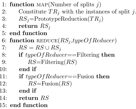
1: functionmap(Number of splitsj)
2: ConstituteT Rj with the instances of split j.
3: RSj=PrototypeReduction(T Rj)
4: returnRSj
5: end function
6: functionreduce(RSj,typeOf Reducer) ⊲ InitiallyRS=∅
7: RS=RS∪RSj
8: if typeOf Reducer==Filteringthen 9: RS=Filtering(RS)
10: end if
11: if typeOf Reducer==Fusionthen 12: RS=Fusion(RS)
[image:10.595.112.337.123.304.2]13: end if 14: returnRS 15: end function
Figure 2: Map and reduce functions
Under this scheme, if the partitioning procedure is directly applied over
T R, the class distribution of each subsetT Rj could be biased to the original
distribution of instances in its corresponding file. As we stated before, a proper stratified partitioning could not be carried out if the size of T R does not fit in the main memory. In order to develop a scheme easily scalable to any number of instances, we previously randomize the entire file. This operation is not time-consuming in comparison with the application of the PR technique and should be applied only once. It does not ensure that every
class is represented proportionally to its number of instances in T R.
How-ever, probabilistically, each chunk should include approximately a number of instances of class ω according to the probability of belonging to this class in the original T R.
When each map has formed its correspondingT Rj, a PR step is performed
using T Rj as the input training data. This step generates a reduced set
RSj. Note that PR techniques may consume different computational times
although they are applied with data sets of similar characteristics. It mainly depends on the stopping criteria of each PR model. Nevertheless, MapReduce starts the reduce phase as the first mapper has finalized. Figure 2 contains the pseudo-code of the map function. This function is basically the application of the PR technique for each training partition.
3.2.2. Reduce phase
The reduce phase will consist of the iterative aggregation of all theRSj as
a single one RS. Figure 2 shows the pseudo-code of the implemented reduce
function. Initially RS =∅. To do so, we propose different alternatives:
• Join: This simple option, based on stratification, concatenates all the
RSj sets into a final reduce set RS. Instruction 7 indicates how the
reduce function progressively joins all the RSj as the mappers finish
their processing. This type of reducer implements the same strategy used in the distributed partitioning procedure that we previously pro-posed [30]. As such, this joining process does not guarantee that the
resulting RS does not contain irrelevant or even harmful instances, but
it is included as a baseline.
• Filtering: This alternative explores the idea of a filtering stage that
removes noisy instances during the formation of RS. This is based on
those prototype selection methods belonging to the edition family of methods [19].
This kind of methods is commonly based on simple heuristics that discard points that are noisy or do not agree with their neighbors. They supply smoother decision boundaries for the NN classifier. In general, edition schemes enhance generalization capabilities by performing a slight reduction of the original training set.
These characteristics are very appropriates for the current stage of our framework. At this stage, the map phase has reduced each partition to a subset of representative instances. To aggregate them into a single
RS set, we do not pursue to reduce more theRS, we focus on
remov-ing noisy instances, if any. Therefore, the reduce function iteratively applies a filtering of the currentRS. It means that as the mappers end
their execution, the reduce function is run and the next RS is
com-puted as the filtered set obtained with its current content and the new
RSj. It is described in instructions 8-10 of Figure 2.
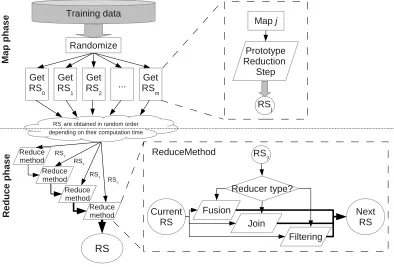
Figure 3: MRPR scheme
fuse all the RSj into a single one, these methods can be very useful to
generate a final set without redundant or very similar prototypes. As in the previous scheme, the fusion phase will be progressively applied
during the creation of RS. Instructions 11-13 of Figure 2 explain how
to apply the fusion phase in the MapReduce framework.
As we have explained, MRPR only uses one single reducer that is run every time that a mapper is completed. With the adopted strategy, the use of a single reducer is computationally less expensive than use more than one. It decreases the Mapreduce overhead (especially network overhead) [40].
As summary, Figure 3 outlines the way of working of the MRPR frame-work, differentiating between the map and reduce phases. It puts emphasis
on how the single reducer works and it forms the finalRS. The resultingRS
will be used as training set for the NN rule to classify the unseen data of the
3.3. Which PR methods are more suitable for the MRPR framework?
In this subsection we explain which kind of PR techniques fit with the proposed MRPR framework in its respective stages. In the map phase, the main prototype reduction process is carried out by a PR technique. Then, depending on the selected reduce type we should select a filtering or a fusion PR technique to combine the resulting reduced sets. In what follows, we discuss which PR techniques are more appropriate for these stages and how to combine them.
All PR algorithms utilize a training set (in our case T Rj) as input and
then return a reduced set RSj. Therefore, all of them could be implemented
in the map phase of MRPR according to the description performed above. However, depending on their characteristics (reduction, accuracy and run-time), we should take into consideration the following aspects to select a proper PR algorithm:
• A very accurate PR technique is desirable. However, in many PR
tech-niques it implies a low reduction rate. A resultingRS with an excessive number of instances can negatively influence in the time needed by the reduce phase.
• The runtime consumption of a PR algorithm will determine the
neces-sary number of mappers in which theT Rset of a given problem should
be divided. Depending on the problem tackled, a very high number
of mappers may result in a non representative subset T Rj from the
original T R.
According to [19, 20], there are six main PR families: edition [41], con-densation [42], hybrid approaches [43], positioning adjustment [25], centroids-based [44] and space splitting [45]. Although there are differences between the methods of each family, most of them perform in a similar way. With these previous notes in mind, we can state the following general recommen-dations:
• Edition-based methods are focused on cleaning the training set by
• Condensation, hybrid and space splitting approaches commonly offer a good trade-off between reduction, accuracy and runtime. Their reduc-tion rate is normally around 60-80%, so that, depending on the problem addressed, the reducer should have a moderate time consumption. For example, we recommend the use of ENN [41] or Depur [46] for filtering reducers and GMCA [44] for fusion.
• Positioning adjustment techniques may offer a very high reduction rate
or even adjustable as a user-defined parameter. These techniques can provide very accurate results in a relatively moderate runtime. To implement these techniques we suggest the inclusion of very accurate reducers, such as ICPL [47] for fusion, because the high reduction rate will allow them to be applied in a fast way.
• Centroid-based algorithms are very accurate, with a moderate
reduc-tion power but (in general) very time-consuming. Although its imple-mentation is feasible and could be useful in some problems, we assume that their use should be limited to the later stage (reduce phase).
As general suggestions to combine PR techniques in the map and reduce phases, we can establish the following rules:
• High reduction rates in the map phase permit very accurate reducers.
• Low reduction rates in the map phase need fast reducers (join, filtering
or a fast fusion).
As commented in the previous section, we propose the use of edition-based methods for the filtering reduce type and centroid-edition-based algorithms to fuse prototypes. In our experiments, we will focus on a simple but effective edition technique: the edited nearest neighbor (ENN) [41]. This algorithm removes an instance from a set of prototypes if it does not agree with the
majority of itsk nearest neighbors. As algorithms to fuse prototype, we will
4. Experimental study
In this section we present all the questions raised with the experimen-tal study and the results obtained. Section 4.1 describes the performance measures used to evaluate the MRPR model. Section 4.2 defines and de-tails the hardware and software support used in our experiments. Section 4.3 shows the parameters of the involved algorithms and the data sets cho-sen. Section 4.4 presents and discusses the results achieved. Finally, Section 4.5 includes additional experiments using different PR techniques within the MRPR model.
4.1. Performance measures
In this work we study the performance of a parallel PR system to improve the NN classifier. Hence, we need several types of measures to characterize the abilities of the proposed approach and its variants. In the following, we briefly describe the considered measures:
• Accuracy: It counts the number of correct classifications regarding the total number of instances classified [4, 48]. In our experiments we will compute training and test classification accuracy.
• Reduction rate: It measures the reduction of storage requirements achieved by a PR algorithm.
ReductionRate= 1−size(RS)/size(T R) (1)
Reducing the stored instances in theT Rset will yield a time reduction to classify a new input sample.
• Runtime: We will quantify the total time spent by MRPR to generate
the RS, including all the computations performed by the MapReduce
framework.
• Test classification time: It refers to the time needed to classify all the instances of T S regarding a givenT R. For PR, it is directly related to the reduction rate.
measures the relation between the runtime of sequential and parallel
versions. If the calculation is executed in c processing cores and it
is considered fully parallelizable, the maximum theoretical speed up would be equal to the number of used cores, according to the the Am-dahl’s Law [49]. With a MapReduce parallelization scheme, each map will correspond to a single core, so that, the number of used mappers determines the maximum attainable speed up. However, due to the magnitude of the data sets used, we cannot run the sequential version of the selected PR technique (SSMA-SFLSDE) because its execution is extremely slow. For this reason, we will take the runtime with the minimum number of mappers as reference time to calculate the speed up. Therefore, the speed up will be computed as:
Speedup= parallel time
parallel time with minimum number of mappers (2)
4.2. Hardware and software used
The experiments have been carried out on twelve nodes in a cluster: The master node and eleven compute nodes. Each one of these compute nodes has the following features:
• Processors: 2 x Intel Xeon CPU E5-2620
• Cores: 6 per processor (12 threads)
• Clock Speed: 2.00 GHz
• Cache: 15 MB
• Network: Gigabit Ethernet (1 Gbps)
• Hard drive: 2 TB
• RAM: 64 GB
HDFS block. The JobTracker is the MapReduce framework master process that manages the TaskTrackers of each compute node. Its responsibilities are maintaining the load-balance and the fault-tolerance in the system, ensuring that all nodes get their part of the input data chunk and reassigning the parts that could not be executed.
The specific details of the software used are the following:
• MapReduce implementation: Hadoop 2.0.0-cdh4.4.0. MapReduce
1 runtime(Classic). Cloudera’s open-source Apache Hadoop distribu-tion [50].
• Maximum maps tasks: 128.
• Maximum reducer tasks: 1.
• Machine learning library: Mahout 0.8.
• Operating system: Cent OS 6.4.
Note that the total number of cores of the cluster is 132. However, the maximum number of map tasks are limited to 128 and one for the reducers.
4.3. Data sets and methods
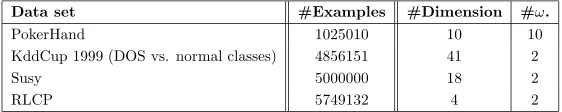
[image:17.595.165.446.546.602.2]In this experimental study we will use four big classification data sets taken from the UCI repository [51]. Table 1 summarizes the main character-istics of these data sets. For each data set, we show the number of examples (#Examples), number of attributes (#Dimension), and the number of classes (#ω).
Table 1: Summary description of the used big data classification
Data set #Examples #Dimension #ω.
PokerHand 1025010 10 10
KddCup 1999 (DOS vs. normal classes) 4856151 41 2
Susy 5000000 18 2
RLCP 5749132 4 2
Table 2: Approximate number of instances in each T Rj subset according to the number
of mappers used.
Number of mappers
Data set 64 128 256 512 1024
PokerHand 12813 6406 3203 1602 801 Kddcup (10%) 6070 3035 1518 759 379 Kddcup (50%) 30351 15175 7588 3794 1897 Kddcup (100%) 60702 30351 15175 7588 3794 Susy 62469 31234 15617 7809 3904 RLCP 71862 35931 17965 8983 4491
training partition, T R). Then, the resulting RS is tested with the current
fold using the NN rule. Test partitions are kept aside during the PR phase in order to analyze the generalization capabilities provided by the generated
RS. Because of the randomness of some operations that these algorithms
perform, they have been run three times per partition.
Aiming to investigate the effect of the number of instances in our MRPR scheme, we will create three different versions of the KDD Cup data set by selecting (randomly) 10%, 50% and 100% of the instances of the original data set. We will denote these versions as Kddcup (10%), Kddcup (50%) and Kddcup (100%). The number of instances of a data set and the number of mappers used in our scheme have a straight relation. Table 2 shows the approximate number of instances per chunk, that is, the size of each T Rj for
MRPR, attending to the number of mappers established. When the number of instances per chunk exceeds twenty thousand, the execution of the PR is not feasible in time. Therefore, we are unable to carry out these experiments. As we stated before, we will focus on the hybrid SSMA-SFLSDE algo-rithm [27] to test the MRPR model. However, in Section 4.5, we will conduct some additional experiments with other PR techniques. Concretely, we will use LVQ3 [52] and RSP3 [45] as pure prototype generation algorithms as well as DROP3 [43] and FCNN [53] as prototype selection algorithms.
Table 3: Parameter specification for all the methods involved in the experimentation
Algorithm Parameters
MRPR Number of mappers = 64/128/256/512/1024. Number of reducers=1 Type of Reduce = Join/Filtering/Fusion.
SSMA-SFLSDE PopulationSFLSDE= 40, IterationsSFLSDE = 500, iterSFGSS =8, iterSFHC=20, Fl=0.1, Fu=0.9 ICLP2 (Fusion) Filtering method = RT2
ENN (Filtering) Number of neighbors = 3, Euclidean distance. NN Number of neighbors = 1, Euclidean distance.
LVQ3 Iterations = 100,alpha= 0.1, WindowWidth=0.2,epsilon= 0.1 RSP3 Subset Choice = Diameter
DROP3 Number of neighbors = 3, Euclidean distance. FCNN Number of neighbors = 3, Euclidean distance. GMCA (Fusion) Number of neighbors = 1, Euclidean distance.
In addition, the NN classifier has been included as baseline limit of per-formance. Table 3 presents all the parameters involved in our experimental study. These parameters have been fixed according to the recommendation of the corresponding authors of each algorithm. Note that our research is not devoted to optimize the accuracy obtained with a PR method over a specific problem. We focus our experiments on the analysis of the behavior of the proposed parallel system. To do so, we will study the influence of the number mappers and type of reduce regarding to the accuracy achieved and the runtime needed. In some of the experiments we will use a higher number of mappers than the available map tasks (128). In these cases, the Hadoop system queues the remaining tasks and they are dispatched as soon as any map task has finished its processing.
A brief description of the used PR methods is:
• SSMA-SFLSDE: This algorithm is a hybridization of prototype
se-lection and generation. First, a prototype sese-lection step is performed based on the memetic algorithm SSMA [32]. This approach makes use of a local search specifically developed for prototype selection. This initial step allows us to find a promising selection of prototypes per
class. Then, its resulting RS is inserted as one of the individuals of
• LVQ3: This method combines strategies to “punish” or “reward” the positioning of a prototype in order to adjust the positioning of a set of initial prototypes (adjustable). Therefore, it is included in the posi-tioning adjustment family.
• RSP3: This technique tries to avoid drastic changes in the form of
de-cision boundaries associated with T Rby splitting it in different subsets according to the highest overlapping degree [45]. As such, it belongs to the family of space-splitting PR techniques.
• DROP3: This model combine a noise-filtering stage and a
decremen-tal approach to remove instances from the original T R set that are
considered as harmful within the nearest neighbors. It is included in the family of hybrid edition and condensation PR techniques.
• FCNN: With an incremental methodology, this algorithm starts by
introducing to the resulting RS the centroids of each class. Then,
a prototype contained in T R will be added according to the nearest
neighbor of each centroid. It belongs to the condensation-based family.
4.4. Exhaustive evaluation of the MRPR framework for the SSMA-SFLSDE method
This section presents and analyzes the results collected in the experi-mental study with the SSMA-SFLSDE method from two different points of view:
• Firstly, we study the accuracy and reduction results obtained with the
three implemented reducers of the MRPR model. We will check the performance achieved in comparison with the NN rule (Section 4.4.1).
• Secondly, we analyze the scalability of the proposed approach in terms
of runtime and speed up (Section 4.4.2).
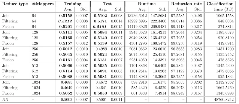
Tables 4, 5, 6 and 7 summarize all the results obtained on the consid-ered data sets. They show training/test accuracy, runtime and reduction rate obtained by the SSMA-SFLSDE algorithm, in our MRPR framework, depending on the number of mappers (#Mappers) and reduce type. For each one of these measures, average (Avg.) and standard deviation (Std.) results are presented (from the 5-fcv experiment). Moreover, the average
Table 4: Results obtained for the PokerHand problem.
Reduce type #Mappers Training Test Runtime Reduction rate Classification
Avg. Std. Avg. Std. Avg. Std. Avg. Std. time (T S)
Join 64 0.5158 0.0007 0.5102 0.0008 13236.6012 147.8684 97.5585 0.0496 1065.1558
Filtering 64 0.5212 0.0008 0.5171 0.0014 13292.8996 222.3406 98.0714 0.0386 848.0034 Fusion 64 0.5201 0.0011 0.5181 0.0015 14419.3926 209.9481 99.1413 0.0217 374.8814
Join 128 0.5111 0.0005 0.5084 0.0011 3943.3628 161.4213 97.2044 0.0234 1183.6378
Filtering 128 0.5165 0.0007 0.5140 0.0007 3949.2838 135.4213 97.7955 0.0254 920.8190 Fusion 128 0.5157 0.0012 0.5139 0.0006 4301.2796 180.5472 99.0250 0.0119 419.6914
Join 256 0.5012 0.0010 0.4989 0.0010 2081.0662 23.6610 96.5655 0.0283 1451.1200
Filtering 256 0.5045 0.0010 0.5024 0.0006 2074.0048 25.4510 97.2681 0.0155 1135.2452 Fusion 256 0.5161 0.0004 0.5151 0.0007 2231.4050 14.3391 98.8963 0.0045 478.8326
Join 512 0.5066 0.0007 0.5035 0.0009 1101.8868 16.6405 96.2849 0.0487 1545.4300
Filtering 512 0.5114 0.0010 0.5091 0.0005 1101.2614 13.0263 97.1122 0.0370 1472.6066 Fusion 512 0.5088 0.0008 0.5081 0.0009 1144.8080 18.3065 98.7355 0.0158 925.1834 Join 1024 0.4685 0.0008 0.4672 0.0008 598.2918 11.6175 95.2033 0.0202 2132.7362 Filtering 1024 0.4649 0.0009 0.4641 0.0010 585.4320 8.4529 96.2073 0.0113 1662.5460 Fusion 1024 0.5052 0.0003 0.5050 0.0009 601.0838 7.4914 98.6249 0.0157 1345.6998
NN – 0.5003 0.0007 0.5001 0.0011 – – – – 48760.8242
Table 5: Results obtained for the Kddcup (100%) problem.
Reduce type #Mappers Training Test Runtime Reduction rate Classification
Avg. Std. Avg. Std. Avg. Std. Avg. Std. time(T S)
Join 256 0.9991 0.0003 0.9993 0.0003 8536.4206 153.7057 99.9208 0.0007 1630.8426 Filtering 256 0.9991 0.0003 0.9991 0.0003 8655.6950 148.6363 99.9249 0.0009 1308.1294 Fusion 256 0.9994 0.0000 0.9994 0.0000 8655.6950 148.6363 99.9279 0.0008 1110.4478 Join 512 0.9991 0.0001 0.9992 0.0001 4614.9390 336.0808 99.8645 0.0010 5569.8084 Filtering 512 0.9989 0.0001 0.9989 0.0001 4941.7682 44.8844 99.8708 0.0013 5430.4020 Fusion 512 0.9992 0.0001 0.9993 0.0001 5018.0266 62.0603 99.8660 0.0006 2278.2806 Join 1024 0.9990 0.0002 0.9991 0.0002 2620.5402 186.5208 99.7490 0.0010 5724.4108 Filtering 1024 0.9989 0.0000 0.9989 0.0001 3103.3776 15.4037 99.7606 0.0011 4036.5422 Fusion 1024 0.9991 0.0002 0.9991 0.0002 3191.2468 75.9777 99.7492 0.0010 4247.8348
NN 0 0.9994 0.0001 0.9993 0.0001 – – – – 2354279.8650
instances of T S with the corresponding RS generated by MRPR.
Further-more, we compare these results with the accuracy and the test classification
time achieved by the NN classifier. It uses the whole T R set to classify all
the instances of T S. In these tables, average accuracies higher or equal than the obtained with the NN algorithm have been highlighted in bold. The best ones in overall, on training and test phases, are stressed in italic.
4.4.1. Analysis of accuracy and reduction capabilities
[image:21.595.117.507.351.469.2]Table 6: Results obtained for the Susy problem.
Reduce type #Mappers Training Test Runtime Reduction rate Classification
Avg. Std. Avg. Std. Avg. Std. Avg. Std. time(T S)
Join 256 0.6953 0.0005 0.7234 0.0004 69153.3210 4568.5774 97.4192 0.0604 30347.0420
Filtering 256 0.6941 0.0001 0.7282 0.0003 66370.7020 4352.1144 97.7690 0.0046 24686.3550 Fusion 256 0.6870 0.0002 0.7240 0.0002 69796.7260 4103.9986 98.9068 0.0040 11421.6820 Join 512 0.6896 0.0012 0.7217 0.0003 26011.2780 486.6898 97.2050 0.0052 35067.5140 Filtering 512 0.6898 0.0002 0.7241 0.0003 28508.2390 484.5556 97.5609 0.0036 24867.5478 Fusion 512 0.6810 0.0002 0.7230 0.0002 30344.2770 489.8877 98.8337 0.0302 12169.2180
Join 1024 0.6939 0.0198 0.7188 0.0417 13524.5692 1941.2683 97.1541 0.5367 45387.6154
Filtering 1024 0.6826 0.0005 0.7226 0.0006 14510.9125 431.5152 97.3203 0.0111 32568.3810 Fusion 1024 0.6757 0.0004 0.7208 0.0008 15562.1193 327.8043 98.7049 0.0044 12135.8233
NN 0 0.6899 0.0001 0.7157 0.0001 – – – – 1167200.3250
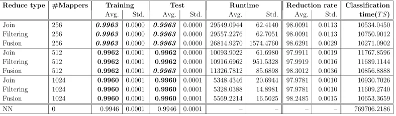
Table 7: Results obtained for the RLCP problem.
Reduce type #Mappers Training Test Runtime Reduction rate Classification
Avg. Std. Avg. Std. Avg. Std. Avg. Std. time(T S)
Join 256 0.9963 0.0000 0.9963 0.0000 29549.0944 62.4140 98.0091 0.0113 10534.0450 Filtering 256 0.9963 0.0000 0.9963 0.0000 29557.2276 62.7051 98.0091 0.0113 10750.9012 Fusion 256 0.9963 0.0000 0.9963 0.0000 26814.9270 1574.4760 98.6291 0.0029 10271.0902
Join 512 0.9962 0.0001 0.9962 0.0000 10093.9022 61.6980 97.9911 0.0019 11767.8596
Filtering 512 0.9962 0.0001 0.9962 0.0000 10916.6962 951.5328 97.9919 0.0016 11689.1144 Fusion 512 0.9962 0.0001 0.9963 0.0000 11326.7812 85.6898 98.3012 0.0036 10856.8888
Join 1024 0.9960 0.0001 0.9960 0.0001 5348.4346 20.6944 97.9781 0.0010 10930.7026
Filtering 1024 0.9960 0.0001 0.9960 0.0001 5328.0388 14.8981 97.9781 0.0010 11609.2740 Fusion 1024 0.9960 0.0001 0.9960 0.0001 5569.2214 16.5025 98.2485 0.0015 10653.3659
NN 0 0.9946 0.0001 0.9946 0.0001 – – – – 769706.2186
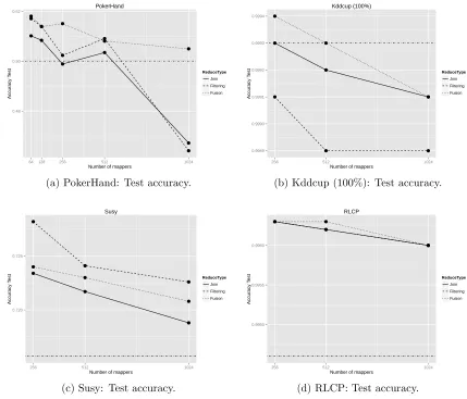
y = AverageAccuracy, to show the accuracy differences between using the
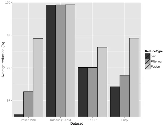
wholeT Ror a generated RS as training data set. In addition, Figure 5 plots
the reduction rates attained by each type of reduce for both problems. In each sub-figure the average reduction rate with 256 mappers has been drawn. According to these graphics and tables we can make several observations from these results:
• Since that within the MRPR framework a PR algorithm does not
[image:22.595.114.508.294.410.2]0.48 0.50 0.52
64 128 256 512 1024
Number of mappers
Accur acy T est ReduceType Join Filtering Fusion PokerHand
(a) PokerHand: Test accuracy.
0.9989 0.9990 0.9991 0.9992 0.9993 0.9994
256 512 1024
Number of mappers
Accur acy T est ReduceType Join Filtering Fusion Kddcup (100%)
(b) Kddcup (100%): Test accuracy.
0.720 0.725
256 512 1024
Number of mappers
Accur acy T est ReduceType Join Filtering Fusion Susy
(c) Susy: Test accuracy.
0.9950 0.9955 0.9960
256 512 1024
Number of mappers
Accur acy T est ReduceType Join Filtering Fusion RLCP
[image:23.595.112.541.139.506.2](d) RLCP: Test accuracy.
Figure 4: Test accuracy results
deteriorated when the problem is divided into 1024 subsets (mappers) in both training and test phases. In Susy data set, the accuracy is gradually deteriorated as the number of mapper is incremented. For the Kddcup (100%) and RCLP problems, their performance is very slightly reduced when the number of mappers is increased (the order of three or four ten-thousandths).
• Nevertheless, it is important to highlight that although the accuracy
97 98 99 100
PokerHand Kddcup (100%) RLCP Susy
Dataset
A
v
er
age reduction (%)
[image:24.595.164.437.129.337.2]ReduceType Join Filtering Fusion
Figure 5: Reduction rate achieved with 256 mappers.
the achieved with the NN rule. In fact, it could be even higher as happens in the cases of PokerHand, Susy and RLCP problems. This situation occurs because PR techniques remove noisy instances from
the T R set that damage the classification performance of the NN rule.
Moreover, PR models typically smooth the decision boundaries between classes that usually rebounds in an improvement of the generalization capabilities (test accuracy).
• When tackling large-scale problems, the reduction rate of a PR
It allows us to classify the T S in a very fast time.
• Independently to the number of mappers and type of reduce, there are
no differences between the results of training a test phases. The parti-tioning process slightly reduces accuracy and reduction rate because of the lack of the whole information. By contrast, this mechanism assists not to fall into the overfitting problem, that is, the overlearning of the training set.
• Comparing the different reduce types, we can check that in general
the fusion approach outperforms to the rest kinds of reducers in most of the data sets. The fusion scheme results in a better training and test accuracy. It is noteworthy that in the case of PokerHand data set, when the other types of reducers decrease their performance, the fusion reducer is able to preserve its accuracy with 1024 mappers. We can also observe that the filtering reducer also provides higher accuracy results than the join approach in PokerHand and Susy problems, while its results are very similar for the Kddcup (100%) and RLCP sets.
• Taking a quick glance at Figure 5, it reveals that the fusion scheme
al-ways reports the higher reduction rate, followed by the filtering scheme. Beside the fusion reducer promotes a higher reduction rate it has shown
the best accuracy. Therefore, it shows that merging the resultant RSj
sets with a fusion or a filtering process provides a better accuracy and reduction rates than a joining phase.
• Considering the results provided by the NN rule and the whole T R,
mappers). These results demonstrate and exemplify the necessity of applying PR techniques to large-scale problems.
4.4.2. Analysis of the scalability
In this part of the experimental study we concentrate on the analysis of runtime and speed up of the MRPR model. As defined in Section 4.3, we divided the Kddcup problem into three sets with different number of instances. We aim to study the influence of the number of instances in the same problem. Figure 6 draws the average runtime (obtained in the 5-fcv experiment) according to the number of mappers used in the problem considered. Moreover, Figure 7 depicts the speed up achieved by MRPR and the fusion reducer.
Note that, as we clarified in Section 4.1, the speed up has been computed
using the runtime with the minimum number of mappers (minMaps) as the
reference time. Therefore, it implies that the speed up does not represent the gain obtained regarding the number of cores. In this chart, the speed up of
MRPR with minMaps in each data set is set as 1. Since the complexity of
SSMA-SFLSDE isO((n·D)2), we cannot expect a quadratic speed up because
the proposed scheme is focused on the number of instances. Furthermore, it is very important to remember that, in the used cluster, the maximum available mappers at the same time is 128 and the rest of tasks are queued.
Figure 8 presents an average runtime comparison between the results obtained in the three versions of the Kddcup problem. It shows for each set its average runtime with 256, 512 and 1024 mappers of the MRPR approach using the reducer based on fusion.
Given these figures and previous tables, we want to outline the following comments:
• Despite the performance showed by the filtering and fusion reducers in
comparison with the joining scheme, all the reduce alternatives spend
very similar runtimes to generate a final RS. It means that although
0 5000 10000 15000
64 128 256 512 1024
Number of mappers
A v er age r untime (s) Reduce Type Join Filtering Fusion PokerHand
(a) PokerHand: Runtime.
4000 6000 8000
256 512 1024
Number of mappers
A v er age r untime (s) Reduce Type Join Filtering Fusion Kddcup (100%)
(b) Kddcup (100%): Runtime.
20000 40000 60000
256 512 1024
Number of mappers
A v er age r untime (s) Reduce Type Join Filtering Fusion Susy
(c) Susy: Runtime.
10000 20000 30000
256 512 1024
Number of mappers
A v er age r untime (s) Reduce Type Join Filtering Fusion RLCP
[image:27.595.116.542.142.500.2](d) RLCP: Runtime.
Figure 6: Average runtime obtained by MRPR
• In Figure 7, we can observe different tendencies depending on the used
0 5 10 15 20 25
256 512 1024
64 128
Number of mappers
Runtime speedup
[image:28.595.168.435.146.350.2]Dataset PokerHand Kddcup (10%) Kddcup (50%) Kddcup (100%) RLCP Susy Runtime speedup
Figure 7: Speed up achieved by MRPR with the fusion reducer
0 2500 5000 7500
256 512 1024
Number of mappers
A
v
er
age r
untime (s)
Dataset Kddcup (10%) Kddcup (50%) Kddcup (100%) Runtime comparison for Kddcup problem
[image:28.595.167.435.415.622.2]MRPR is able to accelerate the processing of PR techniques by
divid-ing in the T R set in a higher number of subsets. As we checked in the
previous section, these speed ups do not fall into a significant accuracy loss.
• Figure 8 illustrates the increment of average runtime when the size of
the same problem is increased. In problems with quadratic complexity, we could expect that with the same number of mappers this increment should be also quadratic. In this figure, we can see that the increment of runtime is much lesser than a quadratic increment. For example, for 512 mappers, MRPR spends 2571.0068 seconds in Kddcup (50%) and 8655.6950 seconds for the full problem. As we can see in Table 2,
the approximate number of instances in each T Rj subset is the double
for Kddcup 100% than Kddcup 50% with 512 mappers. Therefore, its computational cost is not incremented quadratically.
4.5. Experiments on different PR techniques
In this section we perform some additional experiments using four differ-ent PR techniques in the proposed MRPR framework. In these experimdiffer-ents, the number of mappers has been fixed to 64 and we focus on the PokerHand problem. Table 8 shows the results obtained.
Figure 9 presents a comparison across the four techniques within MRPR. Figure 9a depicts the accuracy test obtained by the four techniques using the three reduce types. Figure 9b shows the time needed to classify the test set. In both plots, the results of the NN rule have been presented as baseline. As before, those results that are better than the NN rule have been stressed in bold and the best ones in overall are highlighted in italic.
Observing these results, we can see that the MRPR model works ap-propriately with these techniques. Nevertheless, we can point out several differences in comparison with the results obtained with SSMA-SFLSDE:
• Since LVQ3 is a positioning adjustment method with a high reduction
Table 8: Results obtained for the PokerHand problem with 64 Mappers.
PR technique Reduce type Training Test Runtime Reduction rate Classification
Avg. Std. Avg. Std. Avg. Std. Avg. Std. time (T S)
LVQ3 Join 0.4686 0.0005 0.4635 0.0014 15.3526 0.8460 97.9733 0.0001 841.5352 Filtering 0.4892 0.0007 0.4861 0.0013 17.7602 0.1760 98.6244 0.0101 487.0822 Fusion 0.4932 0.0010 0.4918 0.0012 83.7830 4.8944 99.3811 0.0067 273.4192 FCNN Join 0.4883 0.0008 0.4889 0.0010 39.8196 2.1829 17.7428 0.0241 28232.4110 Filtering 0.5185 0.0006 0.5169 0.0005 5593.4358 23.1895 47.3255 0.0310 19533.5424 Fusion 0.6098 0.0002 0.4862 0.0006 3207.8540 37.2208 72.5604 0.0080 9854.8956 DROP3 Join 0.5073 0.0004 0.5044 0.0014 69.5268 2.5605 77.0352 0.0141 8529.0618 Filtering 0.5157 0.0005 0.5124 0.0013 442.9670 2.6939 81.2203 0.0169 8139.5878 Fusion 0.5390 0.0004 0.5011 0.0005 198.1450 5.2750 92.3467 0.0043 1811.0866 RSP3 Join 0.6671 0.0003 0.5145 0.0007 219.2912 2.8126 53.0566 0.0554 17668.5268 Filtering 0.6491 0.0003 0.5173 0.0008 1898.5854 10.8303 58.8459 0.0280 17181.5448 Fusion 0.5786 0.0004 0.5107 0.0010 1448.4272 60.5462 84.3655 0.0189 5741.6588
NN – 0.5003 0.0007 0.5001 0.0011 – – – – 48760.8242
0.46 0.47 0.48 0.49 0.50 0.51 0.52
DROP3 FCNN LVQ3 RSP3
Method Accur acy test ReduceType Join Filtering Fusion PokerHand
(a) PokerHand: Accuracy Test.
0 10000 20000 30000 40000 50000
DROP3 FCNN LVQ3 RSP3
Method
Classification time (s)
ReduceType Join Filtering Fusion
PokerHand
(b) PokerHand: Classification Time.
Figure 9: Results obtained by MRPR in different PR techniques
• In the previous section we observed that the filtering and fusion stages
provide a greater reduction rate than the join scheme. In this section, we can see that for FCNN, DROP3 and RSP3, their effect is even more accentuated due to the fact that these techniques have a lesser reduc-tion power than SSMA-SFLSDE and LVQ3. Therefore, the filtering and fusion algorithms become more important with these techniques in order to achieve a high reduction ratio.
• The runtime needed by filtering and fusion schemes crucially depends
so that, the runtime of filtering and fusion reducers is greater than the time needed by the join reducer. However, as commented before, the application of these reduces increases the reduction rate, resulting in a faster classification time.
• As commented previously, we have used a fusion reducer based on
GMCA when FCNN, DROP3 and RSP3 are applied. It is noteworthy that this fusion approach has resulted in a faster runtime in compari-son with the filtering scheme. Nevertheless, as we expected, the perfor-mance reached with this fusion reducer, in terms of accuracy, is lower than the obtained with ICLP2 in combination with SSMA-SFLSDE.
• Comparing the results obtained with these techniques and SSMA-SFLSDE,
we can observe that the best accuracy test results is obtained with RSP3 and the filtering scheme (0.5173) with a medium reduction ra-tio (58.8459%). However, the SSMA-SFLSDE algorithm was able to achieve a higher accuracy test (0.5181) using the fusion reducer with a very high reduction rate (99.1413%).
5. Concluding remarks
In this paper we have developed a MapReduce solution for prototype re-duction, denominated as MRPR. The proposed scheme enables to these kinds of techniques to be applied over big classification data sets with promising re-sults. Otherwise, these techniques would be limited to tackle small or medium problems that does not contain more than several thousand of examples, due to memory and runtime restrictions. The MapReduce paradigm has offered a simple, transparent and efficient environment to parallelize the prototype reduction computation. Three different reduce types have been investigated: Join, Filtering and Fusion; aiming to provide more accurate preprocessed sets. We have found that a reducer based on fusion of prototypes permits to obtain reduced sets with higher reduction rates and accuracy performance.
The experimental study carried out has shown that MRPR obtains very competitive results. We have tested its behavior with different kinds of PR techniques, analyzing the accuracy, the reduction rate and the computa-tional cost obtained. In particular, we have studied two prototype selection methods (FCNN and DROP3), two prototype generation (LVQ3 and RSP3) techniques and the hybrid SSMA-SFLSDE algorithm.
• It has allowed us to apply PR techniques in large-scale problems.
• No significant accuracy and reduction losses with very good speed up.
• Its application has resulted in a very big reduction of storage
require-ments and classification time for the NN rule, when dealing with big data sets.
As future work, we consider the study of new frameworks that enable PR techniques to deal with both large-scale and high dimensional data sets.
Acknowledgment
Supported by the Research Projects TIN2011-28488, P10-TIC-6858 and P11-TIC-7765. D.Peralta holds an FPU scholarship from the Spanish Min-istry of Education and Science (FPU12/04902).
References
[1] V. Marx, The big challenges of big data, Nature 498 (7453) (2013) 255– 260.
[2] M. Minelli, M. Chambers, A. Dhiraj, Big Data, Big Analytics: Emerging Business Intelligence and Analytic Trends for Today’s Businesses (Wiley CIO), 1st Edition, Wiley Publishing, 2013.
[3] D. Plummer, T. Bittman, T. Austin, D. Cearley, D. S. Cloud, Defin-ing and describDefin-ing an emergDefin-ing phenomenon. Technical report, Gartner (2008).
[4] E. Alpaydin, Introduction to Machine Learning, 2nd Edition, MIT Press, Cambridge, MA, 2010.
[5] M. Woniak, M. Gra˜na, E. Corchado, A survey of multiple classifier
sys-tems as hybrid syssys-tems, Information Fusion 16 (2014) 3–17.
[7] J. Bacardit, X. Llor`a, Large-scale data mining using genetics-based machine learning, Wiley Interdisciplinary Reviews: Data Mining and Knowledge Discovery 3 (1) (2013) 37–61.
[8] J. Dean, S. Ghemawat, Mapreduce: simplified data processing on large clusters, Communications of the ACM 51 (1) (2008) 107–113.
[9] J. Dean, S. Ghemawat, Map reduce: A flexible data processing tool, Communications of the ACM 53 (1) (2010) 72–77.
[10] S. Ghemawat, H. Gobioff, S.-T. Leung, The google file system, in: Pro-ceedings of the nineteenth ACM symposium on Operating systems prin-ciples, SOSP ’03, 2003, pp. 29–43.
[11] M. Snir, S. Otto, MPI-The Complete Reference: The MPI Core, MIT Press, 1998.
[12] W. Zhao, H. Ma, Q. He, Parallel k-means clustering based on mapre-duce, in: M. Jaatun, G. Zhao, C. Rong (Eds.), Cloud Computing, Vol. 5931 of Lecture Notes in Computer Science, Springer Berlin Heidelberg, 2009, pp. 674–679.
[13] A. Srinivasan, T. Faruquie, S. Joshi, Data and task parallelism in ILP using mapreduce, Machine Learning 86 (1) (2012) 141–168.
[14] Q. He, C. Du, Q. Wang, F. Zhuang, Z. Shi, A parallel incremental extreme svm classifier, Neurocomputing 74 (16) (2011) 2532 – 2540.
[15] I. Palit, C. Reddy, Scalable and parallel boosting with mapreduce, IEEE Transactions on Knowledge and Data Engineering 24 (10) (2012) 1904– 1916.
[16] G. Caruana, M. Li, Y. Liu, An ontology enhanced parallel SVM for scalable spam filter training, Neurocomputing 108 (2013) 45 – 57.
[17] D. Pyle, Data Preparation for Data Mining, The Morgan Kaufmann Series in Data Management Systems, Morgan Kaufmann, 1999.
[19] S. Garc´ıa, J. Derrac, J. Cano, F. Herrera, Prototype selection for nearest neighbor classification: Taxonomy and empirical study, IEEE Transac-tions on Pattern Analysis and Machine Intelligence 34 (3) (2012) 417– 435.
[20] I. Triguero, J. Derrac, S. Garc´ıa, F. Herrera, A taxonomy and experi-mental study on prototype generation for nearest neighbor classification, IEEE Transactions on Systems, Man, and Cybernetics–Part C: Appli-cations and Reviews 42 (1) (2012) 86–100.
[21] J. Derrac, S. Garc´ıa, F. Herrera, IFS-CoCo: Instance and feature se-lection based on cooperative coevolution with nearest neighbor rule, Pattern Recognition 43 (6) (2010) 2082–2105.
[22] J. Derrac, C. Cornelis, S. Garc´ıa, F. Herrera, Enhancing evolutionary instance selection algorithms by means of fuzzy rough set based feature selection, Information Sciences 186 (1) (2012) 73–92.
[23] N. Garc´ıa-Pedrajas, A. de Haro-Garc´ıa, J. P´erez-Rodr´ıguez, A scalable approach to simultaneous evolutionary instance and feature selection, Information Sciences 228 (2013) 150–174.
[24] T. M. Cover, P. E. Hart, Nearest neighbor pattern classification, IEEE Transactions on Information Theory 13 (1) (1967) 21–27.
[25] L. Nanni, A. Lumini, Particle swarm optimization for prototype reduc-tion, Neurocomputing 72 (4-6) (2008) 1092–1097.
[26] I. Triguero, S. Garc´ıa, F. Herrera, IPADE: Iterative prototype adjust-ment for nearest neighbor classification, IEEE Transactions on Neural Networks 21 (12) (2010) 1984–1990.
[27] I. Triguero, S. Garc´ıa, F. Herrera, Differential evolution for optimizing the positioning of prototypes in nearest neighbor classification, Pattern Recognition 44 (4) (2011) 901–916.
[29] J. Derrac, S. Garc´ıa, F. Herrera, Stratified prototype selection based on a steady-state memetic algorithm: a study of scalability, Memetic Computing 2 (3) (2010) 183–199.
[30] I. Triguero, J. Derrac, S. Garc´ıa, F. Herrera, A study of the scaling up capabilities of stratified prototype generation, in: Proceedings of the third World Congress on Nature and Biologically Inspired Computing (NABIC’11), 2011, pp. 304–309.
[31] W.-Y. Chen, Y. Song, H. Bai, C.-J. Lin, E. Chang, Parallel spectral clustering in distributed systems, Pattern Analysis and Machine Intelli-gence, IEEE Transactions on 33 (3) (2011) 568–586.
[32] S. Garc´ıa, J. R. Cano, F. Herrera, A memetic algorithm for evolutionary prototype selection: A scaling up approach, Pattern Recognition 41 (8) (2008) 2693–2709.
[33] N. Garc´ıa-Pedrajas, J. P´erez-Rodr´ıguez, Multi-selection of instances: A straightforward way to improve evolutionary instance selection, Applied Soft Computing 12 (11) (2012) 3590 – 3602.
[34] B. He, W. Fang, Q. Luo, N. K. Govindaraju, T. Wang, Mars: A mapre-duce framework on graphics processors, in: Proceedings of the 17th In-ternational Conference on Parallel Architectures and Compilation Tech-niques, PACT ’08, ACM, New York, NY, USA, 2008, pp. 260–269.
[35] J. Talbot, R. M. Yoo, C. Kozyrakis, Phoenix++: Modular mapreduce for shared-memory systems, in: Proceedings of the Second International Workshop on MapReduce and Its Applications, ACM, New York, NY, USA, 2011, pp. 9–16. doi:10.1145/1996092.1996095.
[36] T. White, Hadoop: The Definitive Guide, 3rd Edition, O’Reilly Media, Inc., 2012.
[37] A. H. Project, Apache hadoop (2013).
URL http://hadoop.apache.org/
[38] A. M. Project, Apache mahout (2013).
[39] C.-L. Chang, Finding prototypes for nearest neighbor classifiers, IEEE Transactions on Computers 23 (11) (1974) 1179–1184.
[40] C.-T. Chu, S. Kim, Y.-A. Lin, Y. Yu, G. Bradski, A. Ng, K. Olukotun, Map-reduce for machine learning on multicore, in: Advances in Neural Information Processing Systems, 2007, pp. 281–288.
[41] D. L. Wilson, Asymptotic properties of nearest neighbor rules using edited data, IEEE Transactions on System, Man and Cybernetics 2 (3) (1972) 408–421.
[42] P. E. Hart, The condensed nearest neighbor rule, IEEE Transactions on Information Theory 18 (1968) 515–516.
[43] D. R. Wilson, T. R. Martinez, Reduction techniques for instance-based learning algorithms, Machine Learning 38 (3) (2000) 257–286.
[44] R. Mollineda, F. Ferri, E. Vidal, A merge-based condensing strategy for multiple prototype classifiers, IEEE Transactions on Systems, Man and Cybernetics B 32 (5) (2002) 662–668.
[45] J. S. S´anchez, High training set size reduction by space partitioning and prototype abstraction, Pattern Recognition 37 (7) (2004) 1561–1564.
[46] J. S. S´anchez, R. Barandela, A. I. Marqu´es, R. Alejo, J. Badenas, Analy-sis of new techniques to obtain quality training sets, Pattern Recognition Letters 24 (7) (2003) 1015–1022.
[47] W. Lam, C. K. Keung, D. Liu, Discovering useful concept prototypes for classification based on filtering and abstraction., IEEE Transactions on Pattern Analysis and Machine Intelligence 14 (8) (2002) 1075–1090.
[48] I. H. Witten, E. Frank, Data Mining: Practical machine learning tools and techniques, 2nd Edition, Morgan Kaufmann, San Francisco, 2005.
[49] G. M. Amdahl, Validity of the single processor approach to achieving large scale computing capabilities, in: Proc. Spring Joint Comput. Conf., ACM, 1967, pp. 483–485.
[50] Cloudera, Cloudera distribution including apache hadoop (2013).
[51] A. Frank, A. Asuncion, UCI machine learning repository (2010).
URL http://archive.ics.uci.edu/ml
[52] T. Kohonen, The self organizing map, Proceedings of the IEEE 78 (9) (1990) 1464–1480.
[53] F. Angiulli, Fast nearest neighbor condensation for large data sets classi-fication, IEEE Transactions on Knowledge and Data Engineering 19 (11) (2007) 1450–1464.
[54] K. V. Price, R. M. Storn, J. A. Lampinen, Differential Evolution A Practical Approach to Global Optimization, Natural Computing Series, 2005.