PROBLEMS
MARCO A. IGLESIAS∗, KUI LIN†, SHUAI LU‡, AND ANDREW M. STUART§
Abstract. Ill-posed inverse problems are ubiquitous in applications. Understanding of algorithms for their solution has been greatly enhanced by a deep understanding of the linear inverse problem. In the applied communities ensemble-based filtering methods have recently been used to solve inverse problems by introducing an artificial dynamical system. This opens up the possibility of using a range of other filtering methods, such as 3DVAR and Kalman based methods, to solve inverse problems, again by introducing an artificial dynamical system. The aim of this paper is to analyze such methods in the context of the linear inverse problem.
Statistical linear inverse problems are studied in the sense that the observational noise is assumed to be derived via realization of a Gaussian random variable. We investigate the asymptotic behavior of filter based methods for these inverse problems. Rigorous convergence rates are established for 3DVAR and for the Kalman filters, including minimax rates in some instances. Blowup of 3DVAR and a variant of its basic form is also presented, and optimality of the Kalman filter is discussed. These analyses reveal a close connection between (iterated) regularization schemes in deterministic inverse problems and filter based methods in data assimilation. Numerical experiments are presented to illustrate the theory.
Key words. Kalman filter, 3DVAR, Statistical inverse problems, Artificial dynamics
AMS subject classifications. 93E11, 65J22, 47A52
1. Introduction In many geophysical applications, in particular in the petroleum industry and in hydrology, distributed parameter estimation problems are often solved by means of ensemble Kalman filters [19]. The basic methodology is to introduce an artificial dynamical system, to supplement this with observations, and to apply the en-semble Kalman filter. The methodology is described in a basic, abstract form, applicable to a general, possibly nonlinear, inverse problem in [11]. In this basic form of the algo-rithm regularization is present due to dynamical preservation of a subspace spanned by the ensemble during the iteration. The paper [12] gives further insight into the develop-ment of regularization for these ensemble Kalman inversion methods, drawing on links with the Levenberg-Marquardt scheme [8]. In this paper our aim is to further the study of filters for the solution of inverse problems, going beyond the ensemble Kalman filter to encompass the study of other filters such as 3DVAR and the Kalman filter itself – see [15] for an overview of these filtering methods. A key issue will be the implementation of regularization with the aim of deriving optimal error estimates.
We focus on the linear inverse problem
y=Au†+η, (1.1)
where A is a compact operator acting between Hilbert spaces X and Y. The exact solution is denoted byu†∈Xandηis a noise polluting the observations. We will consider two situations: Data Model1 where multiple observations are made in the form (1.1); and Data Model 2 where a single observation is made. For modelling purposes we ∗School of Mathematical Sciences, University of Nottingham, UK
†School of Mathematical Sciences, Fudan University, China ([email protected])
‡Corresponding author, School of Mathematical Sciences, Fudan University, China
§Computing and Mathematical Sciences, California Institute of Technology, USA
will assume that the noise η is generated by the GaussianN(0,γ2I), independently in the case of multiple observations. In each case we create a sequence{yn}n≥0; for Data Model 1 the elements of this sequence are i.i.d. N(Au†,γ2I) whilst for Data Model 2 they are yn≡y, with y a single draw from N(Au†,γ2I). The case where multiple
independent observations are made is not uncommon in applications (for example in electrical impedance tomography (EIT, [4]) and, although we do not pursue it here, our methodology also opens up the possibility of considering multiple instances with correlated observational noise, by means of similar filtering-based techniques.
The artificial, partially observed linear dynamical system that underlies our method-ology is as follows:
un=un−1,
yn=Aun+ηn.
(1.2)
Inderivingthe filters we apply to this dynamical system, it is assumed that the{ηn}n≥0 are i.i.d. fromN(0,γ2I). Note, however, that whilst the data sequence{yn}n
≥0we use in Data Model 1 is of this form, the assumption is not compatible with Data Model 2; thus for Data Model 2 we have a form of model errorormodel mis-specification [15].
By studying the application of filtering methods to the solution of the linear inverse problem our aim is to open up the possibility of employing the filtering methodology to (static) inverse problems of the form (1.1), and nonlinear generalizations. We confine our analysis to the linear setting as experience has shown that a deep understanding of this case is helpful both because there are many linear inverse problems which arise in applications, and because knowledge of the linear case guide methodologies for the more general nonlinear problem [6]. The last few decades have seen a comprehensive development of the theory of linear inverse problems, both classically and statistically – see [2, 6] and the references therein. Consider the Tikhonov-Phillips regularization method
argminu 1
2γ2ky−Auk 2
Y+
α
2ku−u0k 2
E
.
This can be reformulated from a probabilistic perspective as the MAP estimator for Bayesian inversion given a Gaussian smoothness prior, with mean u0 and Cameron-Martin space E compactly embedded into X, and a Gaussian noise model as defined above; this connection is eludicated in [13, 5]. We note that from the point of view of Tikhonov-Phillips regularization only the parameter αγ2 is relevant, but that each ofαand γ have separate interpretations in the overarching Bayesian picture, the first as a scaling of the prior precision and the second as observational noise variance. In this paper we deepen the connection between the Bayesian methodology and classical methods.
The recent paper [11] opens up the prospect for a statistical explanation of iterated regularization methods in the form of
un=un−1+Kn(y−Aun−1)
with a general Kalman gain operator Kn. In this paper, we establish the connection
between iterated regularization methods (c.f. [6, 9]) and filter based methods [15] with respect to an artificial dynamic system. More precisely, for a linear inverse problem, we verify that the iterated Tikhonov regularization method
is closely related to filtering methods such as 3DVAR and the Kalman filter when applied to the partially observed linear dynamical system (1.2). The similarity between both schemes provides a probabilistic interpretation of iterated regularization methods, and allows the possibility of quantifying uncertainty via the variance. On the other hand, we will employ techniques from the convergence analysis arising in regularization theories [6] to shed light on the convergence of filter based methods, especially when the linear observation operator is ill-posed. We do not employ Hilbert scales [7, 10, 17, 18] in our analysis as this would lead to a different focus, but their study in this problem would also be of interest.
The paper is organized as follows. We first introduce filter based methods for the artificial dynamics (1.2) in Section 2. Section 3 describes some general useful formulae which are relevant to all the filters we study, and lists our main assumptions on the in-verse problem of interest. In Sections 4 and 5 respectively, detailed asymptotic analyses are given for the Kalman filter method and 3DVAR, for both data models. The final Section 6 presents numerical illustrations confirming the theoretical predictions.
2. Filters For The Artificial Dynamics 2.1. Filter Definitions
Recall the artificial dynamics (1.2), where the observation operatorA also defines the inverse problem (1.1), and{ηn}n≥0 is an i.i.d. sequence withη1∼ N(0,γ2I). The aim of filters is to estimateun given the data {yj}nj=1. In particular, probabilistic fil-tering aims to estimate the probability distribution of the conditional random variable
un|{yj}nj=1.
If we assume that u0∼ N(m0,C0) then the desired conditional random variable is Gaussian, because of the linearity inherent in (1.2), together with the assumed Gaussian structure of the noise sequence{ηn}n≥0. Furthermore the independence of the elements of the noise sequence means that the Gaussian can be updated sequentially in a Marko-vian fashion. If we denote by mn the mean, and byCn the covariance, then we obtain
the Kalman filter updates for these two quantities:
Kn=Cn−1A∗ ACn−1A∗+γ
2I−1
(2.1a)
mn=mn−1+Kn(yn−Amn−1) (2.1b)
Cn= (I−KnA)Cn−1. (2.1c)
The operator Kn is known as the Kalman gainand the inverse of the covariance, the
precision operator C−1
n , may be shown to satisfy
Cn−1=C−
1
n−1+ 1
γ2A
∗A. (2.2)
All of these facts concerning the Kalman filter may be found in Chapter 4 of [15]. Expression (2.2) requires careful justification in infinite dimensions, and this is provided in [1] in certain settings. However we will only use (2.2) as a quick method for deriving useful formulae, not expressed in terms of precision operators, which can be justified directly under the assumptions we make.
A simplification of the Kalman filter method is the 3DVAR algorithm [15] which is not, strictly speaking, a probabilistic filter because it does not attempt to accurately track covariance information. Instead the covariance is fixed in time at
Cn−1=
γ2
for some fixed positive and self-adjoint operator Σ0.The parameterαis a scaling con-stant the inverse of which measures the relative size of the fixed covariance of the filter relative to that of the data. Imposing this simplification on equations (2.1a), (2.1b) gives
Kn≡ K:= Σ0A∗(AΣ0A∗+αI)
−1
(2.4a)
ζn=ζn−1+K(yn−Aζn−1). (2.4b)
It is also helpful to define, from (2.1c),
C ≡γ
2
α(I− KA)Σ0. (2.5)
Notice [6, 16] that the update form (2.4b) looks like a stationary iterated Tikhonov
method (1.3) withAreplaced byAΣ12
0.
Throughout the paper (Kn,mn,Cn) stands for Kalman gain, updated mean and
updated covariance for the Kalman filter method and (K,ζn,C) is the related sequence
of quantities for 3DVAR.
2.2. Asymptotic Behaviour of Filters
We will view the filters as methods for reconstructing the truthu†; in particular we will study the proximity ofmn (for the Kalman filter) and ζn (for 3DVAR) to u† for
various largenasymptotics. Although the assumption in thederivation of the filters is thatyn is an i.i.d. sequence of the form N(Au†,γ2I), we will not always assume that
the data available is of this form; to be precise Data Model 1 is compatible with this assumption whilst Data Model 2 is not.
Recall that Data Model 1 refers to the situation where the data used in the Kalman and 3DVAR filters has the formyn=Au†+ηn, where theηn are i.i.d. N(0,γ2I).Given
such a data sequence we can generate an auxiliary element
¯
y=1
n
n
X
j=1
yj=Au†+
1
n
n
X
j=1
ηj
with ¯η=1nPn
j=1ηj and ¯η∼ N(0,
γ2
nI). The law of large numbers and central limit
theorem thus allows us to consider an inverse problem of the form (1.1) with noise level reduced by a factor of√n.In particular, whennincreases to infinity, the noise and uncertainty in the auxiliary element are removed and one can thus obtain a (generalized) Moore-Penrose inversion by application of a least squares method. We will study, in the sequel, whether the Kalman or 3DVAR filters are able to automatically exploit the decreased uncertainty inherent in an i.i.d. data set of this form.
For Data Model 2 we simply assume that the data used in the filters is of the form yn≡y where y is given by (1.1) with η∼ N(0,γ2I). From the discussion in the
preceding paragraph, we clearly expect less accurate reconstruction in this case. For this data model we may view 3DVAR as a stationary iterated Tikhonov regularization, whilst the Kalman filter is an alternative iterated non-stationary regularization scheme, sinceKnis updated in each step. In addition, the statistical perspective not only allows
In this paper our primary focus is the asymptotic largenbehavior of the Kalman filter method and 3DVAR. More precisely, we are interested in the accurate recovery of the true stateu† when the noise variance vanishes, i.e. γ2→0 for Data Models 1 and 2, or as n→ ∞ for Data Model 1 (by the law of large numbers/central limit theorem discussion above).
To highlight the difficulties inherent in ill-posed inverse problems in this regard, we note the following which is a straightforward consequence of Theorem 4.10 in [15] when specialized to linear problems. Here, and in what follows,k · k denotes both the norm onX and the operator norm fromX into itself.
Proposition 2.1. Consider the 3DVAR algorithm with {yn}n≥1. Assume that there exists a constantLsuch thatkI− KAk ≤L <1and thatkKk<∞.Then, for Data Model 2, it yields
limsup
n→∞
kζn−u†k ≤
kKkkηk
1−L .
Note however, that if the observation operator A is compact or the inversion is ill-posed, the assumption L <1 in the preceding proposition cannot hold. More precisely, the operator I− KA is no longer contractive since the spectrum of the operator KA
clusters at the origin. Our focus in the remainder of the paper will be on such ill-posed inverse problems.
3. Main Assumptions and General Properties of Filters 3.1. Assumptions
Recall that k · k denotes both the norm on X and the operator norm fromX into itself. Throughout C will denote a generic constant, independent of the key limiting quantitiesγ andn. Our main assumption is:
Assumption 1. For both the Kalman filter and the 3DVAR filter, we assume
(i) the variance C0=γ
2
αΣ0 and R(Σ 1/2
0 )⊂ D(A), where α is a positive constant and Σ0 is positive self-adjoint, andΣ−01 is a densely defined unbounded self-adjoint strictly positive operator;
(ii) the forward operatorA satisfies
C−1kΣ
a 2
0xk ≤ kAxk ≤CkΣ
a 2
0xk (3.1)
onX for some constants a >0 and1≤C <∞;
(iii) the initial mean satisfies m0−u†∈ D
Σ−
s 2
0
(or ζ0−u†∈ D
Σ−
s 2
0
) with 0≤s≤
a+ 2;
(iv) the operator Σ0 in item (i) is trace class onX.
We briefly comment on these items. Item (i) allows a well defined operator
B0:=AΣ
1/2
0 (3.2)
which is essential in carrying out our analysis. Item (ii) is often called thelink condition and it connects both operators A and Σ0 (or C0). The third item (iii) is the source condition(regularity) of the true solution [6]. The final item (iv) makesC0a well-defined covariance operator on X [3].
employ the following specific form of items (ii), (iii). Comparison of Assumptions 1 and 2 we see that they are identical ifa=1+22p ands=1+22β.
Assumption 2. Let the varianceC0=γ
2
αΣ0. The operatorsΣ0 andA
∗Ahave the same
eigenfunctions{ei} with their eigenvalues {λi} and{κ2
i}satisfying
λi=i−1−2, C−1i−p≤κi≤Ci−p
for some >0,p >0 andC≥1. Furthermore, by choosing the initial meanm0= 0, the true solution u† with its coordinates {u†,i} in the basis {ei} obeys P∞
i=1(u†
,i)2i2β<∞
and0< β≤1 + 2+ 2p.
3.2. Filter Properties
We start by deriving properties of the Kalman filter method under Data Model 1. Other cases can be simply derived from minor variants of this setting. Recall from (2.1b)
mn= (I−KnA)mn−1+Knyn
and note that
u†= (I−KnA)u†+KnAu†.
Under Data Model 1 we have yn=Au†+ηn and hence the total error en:=mn−u†
satisfies
en= (I−KnA)en−1+Knηn
=
n
Y
j=1
(I−KjA)e0+
n−1
X
j=1
n−1
Y
i=n−j
(I−Ki+1A)
Kn−jηn−j+Knηn (3.3)
:=J1+J2.
Here
J1=
n
Y
j=1
(I−KjA)e0 and
J2=
n−1
X
j=1
n−1
Y
i=n−j
(I−Ki+1A)
Kn−jηn−j+Knηn.
To establish a rigorous convergence analysis, the mean squared error (MSE)Ekmn−
u†k2is of particular interest. Since u† is deterministic and eachη
n is i.i.d Gaussian we
obtain a bias-variance decomposition of the MSE:
Ekmn−u†k2=kJ1k2+EkJ2k2. (3.4)
To proceed further, both termsJ1 andJ2 need to be calibrated more carefully.
We consider the operator I−KnA which appears in both terms. By (2.1c), we
obtain
Cn= (I−KnA)Cn−1=
n
Y
j=1
which is equivalent to
n
Y
j=1
(I−KjA) =CnC0−1. (3.5)
Notice that (2.2) yields
Cn−1=Cn−−11+ 1
γ2A
∗A=C−1
0 +
n
γ2A
∗A. (3.6)
By (3.5) and (3.6) we obtain
n
Y
j=1
(I−KjA) =CnC0−1= (C −1
0 +nA∗A/γ
2)−1C−1 0
=C
1 2
0γ
2(γ2I+nC12
0A ∗AC12
0) −1C−12
0 . (3.7)
We will use this expression (which is well-defined in view of Assumption 1 (i)) and the labelled equations preceding it in this subsection, frequently in what follows.
4. Asymptotic Analysis of the Kalman Filter
In this section we investigate the asymptotic behaviour of the Kalman filter (2.1a)-(2.1c), under Assumption 1. In particular, we are interested in whether we can reproduce the minimax convergence rate. This minimax rate is achieved by adopting Assumption 1 in the diagonal form of Assumption 2.
4.1. Kalman Filter and Data Model1 We present the main results in current subsection.
Theorem 4.1. Let Assumption 1 hold. Then the Kalman filter method (2.1a)-(2.1c)
yields a bias-variance decomposition of the MSE
Ekmn−u†k2≤C
α
n
a+1s +γ
2
αtr(Σ0)
for the Data Model1. Setting α=Ns+as+1 and stopping the dynamic iteration at n=N then gives
EkmN−u†k2≤ C+γ2tr(Σ0)
N−s+sa+1. (4.1)
Theorem 4.2. Let Assumption 2 hold. Then the Kalman filter method (2.1a)-(2.1c)
yields a bias-variance decomposition of the MSE
Ekmn−u†k2≤C
α
n
1+22β+2p
+γ2n−1+22+2pα− 1+2p 1+2+2p
for the Data Model1. Settingα=N1+22(ββ−+2)p and stopping the dynamic iteration atn=N
then gives the following minimax convergence rate:
EkmN−u†k2≤CN−
2β 1+2β+2p.
• (1) Under the Assumption 2 we prove unconditional convergence of the Kalman filter method for any fixed α >0 andγ >0, noticing that both the bias and vari-ance vanish when n goes to infinity. The key ingredient which leads to this unconditional convergence, in comparison with Assumption 1, is that the rate of decay of the eigenvalues of the variance operator Σ0 is made explicit under Assumption 2; this is to be contrasted with the weaker assumption tr(Σ0)<∞ made in Assumption 1 (iv).
• (2) By choosing α depending on the update step N, again with fixed γ, both Theorems 4.1 and 4.2 yield convergence rates in the MSE sense. Indeed in the second case, where we use Assumption 2, the minimax rate of N−1+22ββ+2p is
achieved. This minimax rate may also be achieved from the Bayesian posterior distribution with appropriate tuning of the prior in terms of the (effective) noise size √N [14]; the tuning of the prior is identical to the tuning of the initial condition for the covarianceC0, via choice ofα. ♦ Proof of Theorems 4.1 and 4.2 is straightforward by means of a bias-variance de-composition. Let Assumption 1 (i) hold, noting that thenB0:=AΣ
1/2
0 is well-defined. We thus obtain, by (3.7),
n
Y
i=1
(I−KiA) = Σ
1 2
0α(αI+nB0∗B0)−1Σ −1
2
0 = Σ
1 2
0r1,α n(B
∗ 0B0)Σ
−1 2
0 , (4.2)
where
r1,α n(λ) :=
α n α n+λ
= α
α+nλ. (4.3)
The operator-valued functionr1,α
n (4.3) has been verified to be powerful in the
conver-gence analysis of deterministic regularization schemes – see [16, Ch.2]. In that context the following inequality is useful:
|λtr1,α n(λ)| ≤
α
n
t
, λ∈(0,kB∗0B0k], 0≤t≤1. (4.4)
Following these ideas we obtain the next two lemmas describing the bias and vari-ance error bounds. We leave the proofs of both lemmas to the Appendix. Theorems 4.1 and 4.2 are consequences, by choosing the parameterαappropriately.
Lemma 4.4 (Bias for Kalman filter). Let Assumption 1 (i)-(iii) hold. Then the Kalman filter method (2.1a)-(2.1c) yields
kJ1k2≤C
α
n
a+1s
.
Furthermore, if Assumption 2 is valid, the bias obeys
kJ1k2≤C
α
n
1+22β+2p
.
Lemma 4.5 (Variance for Kalman filter – Data Model 1). Let Assumption 1 (i),
(iv) hold and{ηn} in (1.2) be an i.i.d sequence with η1∼ N(0,γ2I). Then the Kalman filter method (2.1a)-(2.1c) yields
EkJ2k2≤
γ2
Furthermore, if Assumption 2 is valid, the variance obeys
EkJ2k2≤γ2n−
2 1+2+2pα−
1+2p 1+2+2p.
4.2. Kalman Filter and Data Model 2
The key difference between Data Model 2 and Data Model 1 is that, in the case 2, the noisesηnappearing in the expression for the termJ2are identical, rather than i.i.d. mean zero as in case 1. This results in a reduced rate of convergence in case 2 over case 1, as seen in the following two theorems:
Theorem 4.6. Let Assumption 1 hold. Then the Kalman filter method (2.1a)-(2.1c) yields a bias-variance decomposition of the MSE
Ekmn−u†k2≤C
α
n
a+1s +nγ
2
α tr(Σ0)
for the Data Model 2. Fix α= 1 and assume that the noise variance γ2=N−a+s+1 a+1 . If
the dynamic iteration is stopped atn=N then the following convergence rate is valid:
EkmN−u†k2≤(C+ tr(Σ0))N−
s
a+1. (4.5)
Theorem 4.7. Let Assumption 2 hold. Then the Kalman filter method (2.1a)-(2.1c)
yields a bias-variance decomposition of the MSE
Ekmn−u†k2≤C
α
n
1+22β+2p
+γ2n α
1+21+2+2pp
for the Data Model2. Fixα= 1 and assume that the noise varianceγ2=N−1+2β+2p 1+2+2p.If
the dynamic iteration is stopped at n=N then the following convergence rate is valid:
EkmN−u†k2≤CN−
2β 1+2+2p.
Both convergence rates in Theorems 4.6 and 4.7 are of the same order since the variance has been tuned to scale in the same way as the bias by choosing to stop the dynamic iteration at N, depending on γ1, appropriately. In comparison with the convergence rates in Theorems 4.1 and 4.2, the ones in this section under Data Model 2 require small noiseγ; those in the preceding subsection do not because multiple obser-vations, with additive independent noise, are made of Au†.Proof of the two preceding theorems is straightforward: the J1 terms is analyzed as in the preceding subsection and theJ2 term must be carefully analyzed under the assumptions of Data Model 2. The key new result is stated in the following lemma, whose proof may be found in the Appendix.
Lemma 4.8 (Variance for Kalman filter method – Data Model 2). Let Assumption 1 hold and each observationyn≡ybe fixed. Then the Kalman filter method (2.1a)-(2.1c)
yields
EkJ2k2≤
nγ2
α tr(Σ0).
Furthermore, if Assumption 2 is valid, the variance obeys
EkJ2k2≤γ2
n
α
1+21+2+2pp
5. Asymptotic Analysis of 3DVAR 5.1. Classical 3DVAR
The mean of the 3DVAR algorithm is given by (2.4b) and has the form
ζn= (I− KA)ζn−1+Kyn.
Furthermore
u†= (I− KA)u†+KAu†.
If we defineεn=ζn−u† then we obtain, sinceyn=Au†+ηn,
εn= (I− KA)εn−1+Kηn
= (I− KA)nε0+
n−1
X
j=0
(I− KA)jKηn−j
withε0:=ζ0−u†. We further derive
(I− KA)n= Σ 1 2
0(α(αI+B ∗
0B0)−1)nΣ −1
2
0 = Σ
1 2
0rn,α(B∗0B0)Σ −1
2
0 ,
by inserting the definition of the Kalman gain (2.4a), and by assuming Assumption 1 (i). The operator-valued functionrn,α(·) is defined
rn,α(λ) :=
α
α+λ
n
.
Similarly to the analysis of the Kalman filter, we derive
εn= (I− KA)nε0+
n−1
X
j=0
(I− KA)jKηn−j (5.1)
= Σ12
0rn,α(B0∗B0)Σ −1
2
0 ε0+
n−1
X
j=0
(I− KA)jKηn−j
:=I1+I2.
Thus, the MSE takes the bias-variance decomposition form
Ekζn−u†k2=Ekεnk2=kI1k2+EkI2k2.
This leads to the following two theorems:
Theorem 5.1. Let Assumption 1 hold. Then 3DVAR filter (2.4a)-(2.4b) yields a
bias-variance decomposition of the MSE
Ekζn−u†k2≤C
α
n
a+1s +Cγ
2lnn
α tr(Σ0)
for the Data Model1. Setting α=Ns+as+1 and stopping the dynamic iteration at n=N then gives
Ekζn−u†k2≤C 1 +γ2tr(Σ0)N−
s
Theorem 5.2. Let Assumption 2 hold. Then 3DVAR filter (2.4a)-(2.4b) yields a bias-variance decomposition of the MSE
Ekζn−u†k2≤C
α
n
1+22β+2p
+Cγ2α−1+21+2+2pp
for the Data Model 1. Setting α=N1+2+22ββ+2p and stopping the dynamic iteration at
n=N then gives
EkζN−u†k2≤C 1 +γ2
N−1+2+22ββ+2plnN.
Remark 5.3. The decay rate at the end of the preceding Theorem is the same as that
in Theorem 5.1 if a=1+22p and s=1+22β. This is the setting in which Assumptions 1 and 2 are identical.
The preceding two theorems show that, under Data Model 1 and for any fixed α, the (bound on the) MSE of the 3DVAR filter blows up logarithmically as n→ ∞under Assumption 1, and is asymptotically bounded for Assumption 2. In contrast, for the Kalman filter method the MSE is asymptotically bounded or unconditionally converges in nunder the same assumptions – see Theorems 4.1 and 4.2.
With optimal choice ofαin terms of the stopping time of the dynamic iteration at
n=N, comparison of the convergence rates in Theorems 4.1 and 5.1 (or Theorems 4.2 and 5.2) shows that the Kalman filter outperforms 3DVAR, but only by a logarithmic factor (or a H¨older factor). For simplicity we only analyze and discuss Data Model1for 3DVAR filter under the additional Assumption 2; as for Data Model 2 one can derive consequences similar to those in the preceding section in an analogous manner.
We emphasize that in the case of deterministic iterated Tikhonov regularization it is possible to use infinite dynamic observations to overcome the restriction s≤a+ 2 in Assumption 1, for 3DVAR in the case of a constant regularization parameterα= 1; this
is related to the Lardy’s method [9]. ♦
We now study Data Model 2 and 3DVAR. We consider only Assumption 1; however the reader may readily extend the analysis to include Assumption 2. In the case of Data Model 2, both the Kalman and 3DVAR filters have the same error bounds:
Theorem 5.4. Let Assumption 1 hold. Then the 3DVAR algorithm (2.4a)-(2.4b) yields
a bias-variance decomposition of the MSE
Ekζn−u†k2≤C
α
n
a+1s +nγ
2
α tr(Σ0)
for the Data Model 2. Fix α= 1 and assume that the noise variance γ2=N−a+a+1s+1. If the dynamic iteration is stopped atn=N then the following convergence rate is valid:
Ekζn−u†k2≤(C+ tr(Σ0))N−
s
a+1. (5.3)
Lemma 5.5 (Bias for 3DVAR).Let Assumption 1(i)-(iii)hold. Then 3DVAR (2.4)
yields
kI1k2≤C
α
n
a+1s
.
Furthermore, if Assumption 2 is valid, the bias obeys
kI1k2≤C
α
n
1+22β+2p
.
Lemma 5.6 (Variance for 3DVAR - Data Model 1). Let Assumption 1(i),(iv)hold
and each noise ηn in (1.2) i.i.d. generated byN(0,γ2I). Then 3DVAR (2.4) yields
EkI2k2≤C
γ2lnn
α tr(Σ0)
for Data Model1. Furthermore, if Assumption 2 is valid, the variance obeys
EkI2k2≤Cγ2α−
1+2p 1+2+2p
and simultaneously
EkI2k2≤C
γ2lnn
α .
Lemma 5.7 (Variance for 3DVAR - Data Model 2). Let Assumption 1 hold and each observationyn≡y be fixed. Then 3DVAR (2.4) yields
EkI2k2≤
nγ2
α tr(Σ0)
for Data Model2.
5.2. Variant of 3DVAR for Data Model 1 Recall that the 3DVAR update form (2.4b) looks like a stationary iterated Tikhonov method (1.3) [6, 16], withA
re-placed byAΣ 1 2
0 and with a fixed parameter α. The non-stationary iterated Tikhonov regularization, with varying α, has been proven to be powerful in deterministic in-verse problems [9]. We generalize this method to the 3DVAR setting. Furthermore we demonstrate that, for Data Model 1, it is possible to see blow-up phenomena with this algorithm.
Starting from the classical form of the 3DVAR filter as given in (2.4a), (2.4b), (2.5) we propose a variant method in whichαvaries withn. We obtain
Kn:= Σ0A∗(AΣ0A∗+αnI)−1 (5.4a)
vn:=vn−1+Kn(yn−Avn−1) (5.4b)
Cn:=
γ2
αn
(I− KnA)Σ0. (5.4c)
If we definen=vn−u† then we obtain, analogously to the derivation of (3.3) and
(5.1), the bias-variance decomposition as follows:
n= (I− KnA)n−1+Knηn
=
n
Y
j=1
(I− KjA)0+
n−1
X
j=1
n−1
Y
i=n−j
(I− Ki+1A)
Kn−jηn−j+Knηn
with
0=v0−u†;
I1=
n
Y
j=1
(I− KjA)0;
I2=
n−1
X
j=1
n−1
Y
i=n−j
(I− Ki+1A)
Kn−jηn−j+Knηn.
By calibrating both termsI1, I2 carefully, we obtain the following blow-up result, proved in the Appendix. Although the result only provides an upper bound, numerical evidence does indeed show blow-up in this regime.
Theorem 5.8. Let Assumption 1 hold and letαn be a sequence satisfying α1
n≤cσ˜ n−1,
with constant˜c, forσn:=P n j=1
1
αj.Then the variant EnKF method (5.4a)-(5.4c) yields
a bias-variance decomposition of the MSE
Ekvn−u†k2≤C
σ−
s a+1
n +γ2tr(Σ0)σn
for Data Model 1. In particular, the geometric sequence αn:=αqn−1 with α >0 and
0< q <1 yields
Ekvn−u†k2≤C q
s
a+1n+γ2tr(Σ0)q−n.
6. Numerical Illustrations
In this section we provide numerical results which display the capabilities of 3DVAR and Kalman filter for solving linear inverse problems of the type described in Section 1. In addition, we verify numerically some of the theoretical results from Section 4 and Section 5.
6.1. Set-Up
We consider the two-dimensional domain Ω = [0,1]2 and define the operators
A= (−4)−1, Σ0=A2 (6.1)
with
D(4) =nv∈H2(Ω)| ∇v·n= 0 on∂Ω,
Z
Ω
v= 0o.
With this domain −4 is positive, self-adjoint and invertible. Note that (3.1) from Assumption 1 is satisfied witha= 1 andC= 1. In the following subsections we produce synthetic data from a true functionu† that we generate as a two-dimensional random field drawn from the Gaussian measureN(0,Σ) with covariance
Σ =−4+ 1 10I
−(2s+1)
(6.2)
u† yields u†∈ Ht for all 0< t <2s. Therefore, for discussion of the present experiments
we simply assume that u†−m0∈ D(Σ−
s/2
0 ) =H2s. Consequently, in order to satisfy Assumption 1 (iii) we needssuch that 0< s≤a+ 2 = 3. Note that operator Σ0in (6.1) satisfies Assumption 1 (iv).
The numerical generation of u† is carried out by means of the Karhunen-Loeve decomposition of u† in terms of the eigenfunctions of Σ which, from the definition of
D(Σ), are cosine functions. We recall that for the application of the Kalman Filter and 3DVAR with Data Model 1 we need to generateN instances of synthetic data{yn}N
n=1 where N is the maximum number of iterations of the scheme. Below we discuss the selection of such N. The aforementioned synthetic data are generated by means of
yn≡Au†+ηn withηn∼N(0,γ2I) andγspecified below. For Data Model 2 we produce
synthetic data simply by settingyn≡y=Au†+η withη∼N(0,γ2I). In order to avoid
inverse crimes [13], all synthetic data used in our experiments are generated on a finer grid (120×120 cells) than the one (of 60×60 cells) used for the inversion. We use splines to interpolate synthetic data on the coarser grid that we use for the application of the filters.
For both 3DVAR and Kalman filter with Data Model 1, we fix the number of iterationsN for the scheme and consider the selectionα=Ns+1+s a stated in Theorem
4.1 and Theorem 5.1. Provided that the filters are stopped according ton=N, these theorems ensure the convergence rates in (4.1) and (5.2) that we verify numerically in the following subsection. For Data Model 2, Theorem 4.6 and Theorem 5.4 suggest that convergence rates (4.5) and (5.3) are satisfied forα= 1 and provided thatγ2=N−a+s+1
a+1 .
The latter equality provides an expression for the number of iterationsN=N(γ) that we may view as a stopping criterion, extended from the deterministic setting for these filtering algorithms applied to Data Model 2. In Algorithm 1 we summarize the Kalman filter and 3DVAR schemes applied to both data models.
Algorithm 1. Kalman Filter/3DVAR (Data Model1/Data Model 2)
Let
N=
(
fix integer selected a priori for Data Model1
round(γ−2(a+as+1)+1) for Data Model 2
and
α=
Ns+1+s a for Data Model 1
1 for Data Model 2
Forn= 1,...,N, update mn−1 andCn−1 as follows
mn=mn−1+Kn(yn−Amn−1)
Cn=
(I−KnA)Cn−1,for Kalman Filter
Cn−1, for 3DVAR where
Kn=Cn−1A∗ ACn−1A∗+γ
2I−1
.
and where we recall that
yn=
Au†+ηn for Data Model1
y for Data Model2
6.2. Using Kalman Filter and 3DVAR for solving linear inverse problems
In this subsection we demonstrate how the filters under consideration in the iterated framework described in Algorithm 1 can be used, with Data Model 1 and Data Model 2, to solve the linear inverse problem presented in Section 1. Let us consider the truthu†
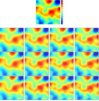
displayed in Figure 6.1 (top) generated, as described in subsection 6.1, from a Gaussian measure with covariance (6.2) and s= 1. Synthetic data are generated as described above with three different choices of γ that yield noise levels of approximately 1%, 2.5%, and 5% of the norm of the noise free data (i.e. Au†).
We apply Algorithm 1 to this synthetic data generated both for the application of Data Model 1 and Data Model 2. For Data Model 1 we consider a selection of
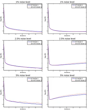
N= 25. Algorithm 1 states that the these schemes should be stopped at the leveln=N. However, in order to observe the performance of these schemes, in these experiments we allowed for a few more iterations. In the left column of Figure 6.2 we display the plots of the error w.r.t the truth of the estimatormn as a function of the iterations, i.e.
E(mn)≡ kmn− Pu†k
wherePu†denotes the interpolation ofu†on the coarse grid used for the inversion. Note that the error w.r.t. the truth of the estimates produced by both schemes decreases monotonically. Interestingly, the value at the final iteration displayed in these figures is approximately the same for all these experiments independently of the noise level. Moreover, the stability of the scheme does not seem to depend on the early termination of the scheme. In addition, we note that both Kalman filter and 3DVAR exhibit very similar performance in terms of reducing the error w.r.t the truth. However, for larger noise levels we observe small fluctuations in the error obtained with 3DVAR.
In Figure 6.1 we display the estimatesmnobtained with 3DVAR with Data Model 1
at iterationsn= 1,10,20,30 for noise levels (determined by the choice ofγ) of 1% (top-middle), 2.5% (middle-bottom) and 5% (bottom). We can visually appreciate from Figure 6.1 that the estimates obtained at the final iteration n= 30 are indeed similar one to another even though the one in the bottom row was computed by inverting data five times noisier than the one in the first row. Similar estimates (not shown) were obtained with the Kalman filter for Data Model 1.
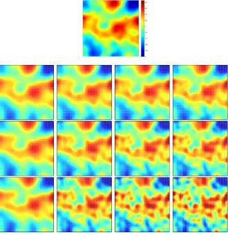
For Data Model 2, the selection ofγ corresponding to noise levels of 1%, 2.5%, and 5% yields a maximum number of iterationsN= 20,6,3 respectively. Clearly, for Data Model 2, smaller observational noise results in schemes that can be iterated longer, presumably achieving more accurate estimates. Similarly to Data Model 1, we are required to stop the algorithm atn=N. However, for the purpose of this study we iterate untiln= 30. In the right column of Figure 6.2 we display the plots of the error w.r.t the truth of mn. In contrast to Data Model 1, we observe that the error w.r.t
the truth increases for n > N. In other words, the Kalman filter and 3DVAR, when applied to Data Model 2, need to be stopped at n=N in order to stabilize the scheme and obtain accurate estimates of the truth. Moreover, stopping the scheme at n=N
results in estimates whose accuracy increases with smaller noise levels. Clearly, in the small noise limit, both data models tend to exhibit similar behaviour. In Figure 6.3 we displaymnobtained from 3DVAR applied to Data Model 2 at iterationsn= 1,10,20,30
is not sufficiently small. The results from this subsection show that the reduction in the variance of the noise due to the law of large numbers and central limit theorem effect in Data Model 1 produces more accurate algorithms. Although Data Model 1 requires multiple instances of the data, in some applications such as in EIT [4], the data collection can be repeated multiple times in order to obtain these data.
Fig. 6.1.Top: truthu†. Top-middle, bottom-middle and bottom: Estimates obtained with 3DVAR and Data Model 1 at iterations (from left to right) 1, 10, 20, 30) for noise levels of1%(top-middle),
2.5%(bottom-middle) and5%(bottom) .
6.3. Numerical verification of convergence rates
In this subsection we test the convergence rates from Theorems 4.1, 5.1, 4.6, and 5.4. For the verification of each of these rates we let Σ := Σsdenote the covariance from
(6.2), and we consider 20 experiments corresponding to different truthsu† generated from N(0,Σs) with the four selections of s= 1,2,3,4. Note that Assumption 1 (iii) is
satisfied only fors≤3. Again, for Data Model 1 we generate synthetic data for each of the truths and for as many iterations used for the application of both schemes. Inverse crimes are avoided as described in subsection 6.1.
5 10 15 20 25 30 0.5
1 1.5 2 2.5 3 3.5
iterations
log (E)
1% noise level
KF Model 1 3DVAR Model 1
5 10 15 20 25 30
0.5 1 1.5 2 2.5 3 3.5
iterations
log (E)
1% noise level
KF Model 2 3DVAR Model 2
5 10 15 20 25 30
0.5 1 1.5 2 2.5 3 3.5
iterations
log (E)
2.5% noise level
KF Model 1 3DVAR Model 1
5 10 15 20 25 30
0.5 1 1.5 2 2.5 3 3.5
iterations
log (E)
2.5% noise level
KF Model 2 3DVAR Model 2
5 10 15 20 25 30
0.5 1 1.5 2 2.5 3 3.5
iterations
log (E)
5% noise level
KF Model 1 3DVAR Model 1
5 10 15 20 25 30
0.5 1 1.5 2 2.5 3 3.5
iterations
log (E)
5% noise level
[image:17.504.105.403.62.439.2]KF Model 2 3DVAR Model 2
Fig. 6.2. log Error with respect to the truth vs iterations of 3DVAR and Kalman filter applied to Data Model 1 (left) and Data Model 2 (right) for different noise levels
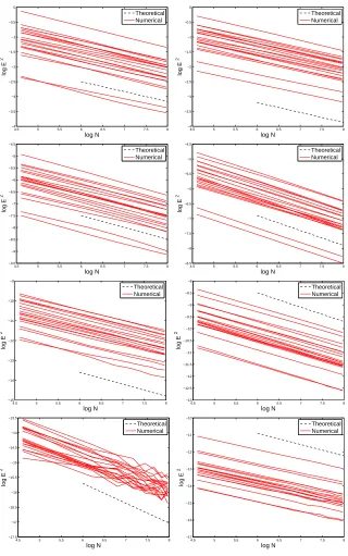
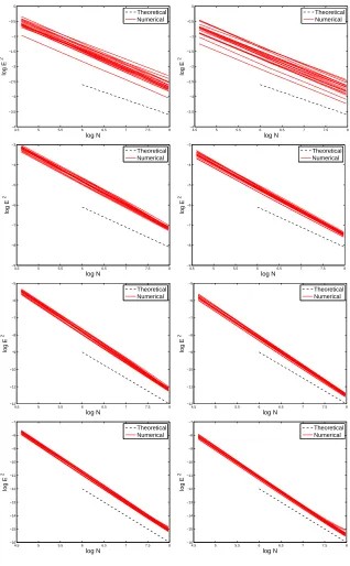
case of Data Model 1 is straightforward. For each of the set of synthetic data associated to each of the 20 truthsu† previously mentioned, we fixγ= 5×10⁻⁴. For eachN (with
N={100,...,3000}) we run Algorithm 1, stop the schemes at n=N and record the
value ofkζN−u†k2. In the right (resp. left) Figure 6.4 we display a plot ofkζN−u†k2
vs logN for the Kalman filter (resp. 3DVAR) for each of the set of 20 experiments associated to different truths (red solid lines) generated as described above with (from top to bottom)s= 1,2,3,4. From Theorem 4.1 we note that the corresponding slopes of the convergence rates should be approximately given by− s
s+1+a. For Theorem 5.1
there is an additional term of logN, but this is of course negligible compared to the algebraic decay and we ignore it for the purposes of this discussion. For comparison, a line (black dotted) with slope − s
s+1+a is displayed in Figure 6.4.
Fig. 6.3.Top: truthu†. Top-middle, bottom-middle and bottom: Estimates obtained with 3DVAR and Data Model 2 at iterations (from left to right) 1, 10, 20, 30) for noise levels of1%(top-middle),
2.5%(bottom-middle) and5%(bottom)
.
γ, in order to obtain convergence. However, for the purpose of the verification of the aforementioned convergence rates we defineγ in terms ofN by means of the same expressions. In other words, for eachN (N={100,...,3000}) we produce synthetic data
(or each of the 20 truths) withη∼N(0,γ2) andγ=N−2(a+as+1)+1. We then run Algorithm 1 and stop the schemes at n=N. In the right (resp. left) Figure 6.5 we display a plot ofkζN−u†k2 vs logN for the Kalman filter (resp. 3DVAR) for each of the set of
20 experiments associated to different truths (red solid lines) generated as before with (from top to bottom)s= 1,2,3,4. We again include a line (black dotted) with slope of
− s
a+1 which is the asymptotic behavior predicted by Theorems 4.6 and 5.4.
rates are slightly smaller than the theoretical ones. In this case (s= 4) there are also fluctuations of the error w.r.t. the truth obtained with 3DVAR. These fluctuations may be associated with the fact that since for the error w.r.t. the truth is very small for sufficiently large iterations and for Data Model 1 the noise level is fixed a priori (recall
γ= 5×10⁻⁴). However, for the Kalman filter these fluctuations are not so evident; presumably updating the covariance has a stabilizing effect. For Data Model 2, asN
increases, the correspondingγ decreases and so these fluctuations in the error are non existent.
7. Conclusions
• We have presented filter based algorithms for the linear inverse problem, based on introduction of an artificial dynamic. This results in methods which are closely related to iterated Tikhonov-type regularization. Two data scenarios are considered, one (Data Model 1) involving multiple realizations of the data, with independent noise; the other (Data Model 2) involving a single realization of the data; both are relevant in applications.
• We present theoretical results demonstrating convergence of the algorithms in the two data scenarios. For multiple realizations of the noisy the convergence is induced by the inherent averaging present in the iterated method, and the link to the law of large numbers and central limit theorem. For the single instance of data the small observational noise limit must be considered.
• For both Data Model 1 and Data Model 2 the Kalman Filter and 3DVAR produced very similar results for relatively small N (N <100). In practice it is clear that 3DVAR is preferable as the Kalman filter requires covariance updates which may be impractical for large scale models. However, updating the covariance in the Kalman filter seems to have an stabilizing effect in the error w.r.t the truth.
• For Data Model 1 the level of accuracy of the estimator is independent of the noise level. Moreover, the stability of the scheme is not conditioned to the early termination of the scheme. In contrast, for Data Model 2 we need to stop at
n=N to avoid an increase in the error w.r.t the truth. Again, this illustrates that, whenever multiple instances of the data are available, Data Model 1 offers a more stable and accurate framework for solving the inverse problems under consideration.
• The theoretical results from this work are verified numerically whenever the assumptions of the theory are satisfied.
Acknowledgements. Shuai Lu is supported by NSFC No.11522108, Shanghai Municipal Education Commission No.16SG01 and Special Funds for Major State Basic Research Projects of China (2015CB856003). Andrew M. Stuart is funded by EPSRC (under the Programme Grant EQUIP), DARPA (under EQUiPS) and The Office of Naval Research under Award Number N000141712079.
REFERENCES
[1] Agapiou S.; Larsson S. and Stuart A. M.: Posterior contraction rates for the Bayesian approach to linear ill-posed inverse problems, Stochastic Process. Appl. 123 (2013), no. 10, 3828–3860. [2] Bissantz N.; Hohage T.; Munk A. and Ruymgaart F.:Convergence rates of general regularization
methods for statistical inverse problems and applications, SIAM J. Numer. Anal., 45 (2007), 2610–2636.
4.5 5 5.5 6 6.5 7 7.5 8 −4 −3.5 −3 −2.5 −2 −1.5 −1 −0.5 0 log N log E 2 Theoretical Numerical
4.5 5 5.5 6 6.5 7 7.5 8 −4 −3.5 −3 −2.5 −2 −1.5 −1 −0.5 0 log N log E 2 Theoretical Numerical
4.5 5 5.5 6 6.5 7 7.5 8 −9.5 −9 −8.5 −8 −7.5 −7 −6.5 −6 −5.5 −5 −4.5 log N log E 2 Theoretical Numerical
4.5 5 5.5 6 6.5 7 7.5 8 −8.5 −8 −7.5 −7 −6.5 −6 −5.5 −5 −4.5 log N log E 2 Theoretical Numerical
4.5 5 5.5 6 6.5 7 7.5 8 −15 −14 −13 −12 −11 −10 −9 log N log E 2 Theoretical Numerical
4.5 5 5.5 6 6.5 7 7.5 8 −13 −12.5 −12 −11.5 −11 −10.5 −10 −9.5 −9 −8.5 −8 log N log E 2 Theoretical Numerical
4.5 5 5.5 6 6.5 7 7.5 8 −17.5 −17 −16.5 −16 −15.5 −15 −14.5 −14 −13.5 log N log E 2 Theoretical Numerical
[image:20.504.94.414.81.592.2]4.5 5 5.5 6 6.5 7 7.5 8 −17 −16 −15 −14 −13 −12 −11 −10 log N log E 2 Theoretical Numerical
Fig. 6.4.Convergence rates for 3DVAR (Left) and Kalman Filter (Right) with Data Model 1 and synthetic data generated from 20 different truths with regularityH2swiths(from top to bottom) 1,2,3
4.5 5 5.5 6 6.5 7 7.5 8 −4 −3.5 −3 −2.5 −2 −1.5 −1 −0.5 0 log N log E 2 Theoretical Numerical
4.5 5 5.5 6 6.5 7 7.5 8 −4 −3.5 −3 −2.5 −2 −1.5 −1 −0.5 0 log N log E 2 Theoretical Numerical
4.5 5 5.5 6 6.5 7 7.5 8 −9 −8 −7 −6 −5 −4 −3 log N log E 2 Theoretical Numerical
4.5 5 5.5 6 6.5 7 7.5 8 −9 −8 −7 −6 −5 −4 −3 log N log E 2 Theoretical Numerical
4.5 5 5.5 6 6.5 7 7.5 8 −12 −11 −10 −9 −8 −7 −6 −5 log N log E 2 Theoretical Numerical
4.5 5 5.5 6 6.5 7 7.5 8 −12 −11 −10 −9 −8 −7 −6 −5 log N log E 2 Theoretical Numerical
4.5 5 5.5 6 6.5 7 7.5 8 −16 −15 −14 −13 −12 −11 −10 −9 −8 −7 log N log E 2 Theoretical Numerical
[image:21.504.94.412.82.596.2]4.5 5 5.5 6 6.5 7 7.5 8 −16 −15 −14 −13 −12 −11 −10 −9 −8 −7 log N log E 2 Theoretical Numerical
Fig. 6.5.Convergence rates for 3DVAR (left) and Kalman Filter (right) with Data Model 2 and synthetic data generated from 20 different truths with regularityH2swiths(from top to bottom) 1,2,3
[4] Borcea L.,Electrical impedance tomography., Inverse Problems Series 18(6), 2002.
[5] Dashti M.; and Stuart A. M.: The Bayesian approach to inverse problems. To appear in The Handbook of Uncertainty Quantification, Editors R. Ghanem, D. Higdon and H. Owhadi, Springer, 2016. arXiv:1302.6989
[6] Engl H. W.; Hanke M. and Neubauer A.: Regularization of inverse problems, Mathematics and its Applications, vol. 375, Kluwer Academic Publishers Group, Dordrecht, 1996.
[7] Goldenshluger A. and Pereverzev S. V.: On adaptive inverse estimation of linear functionals in Hilbert scales, Bernoulli, 9 (2003), 783–807.
[8] Hanke M.: A regularizing Levenberg-Marquardt scheme, with applications to inverse groundwater filtration problems.Inverse Problems, 13 (1997), 79–95.
[9] Hanke M. and Groetsch C. W.: Nonstationary iterated Tikhonov regularization, Journal of Opti-mization Theory and Applications 98 (1998), no. 1, 37–53.
[10] Hohage T. and Pricop M.:Nonlinear Tikhonov regularization in Hilbert scales for inverse bound-ary value problems with random noise, Inv. Probl. Imag., 2 (2008), 271–290.
[11] Iglesias M. A.; Law K. J. and Stuart A. M.: Ensemble Kalman methods for inverse problems, Inverse Problems 29 (2013), no. 4, 045001.
[12] Iglesias M. A.: A regularizing iterative ensemble Kalman method for PDE-constrained inverse problems. To apper in Inverse Problems. arXiv:1505.03876.
[13] Kaipio J. and Somersalo E.:Statistical and computational inverse problems. Applied Mathematical Sciences, 160. Springer-Verlag, New York, 2005.
[14] Knapik B. T.; Van Der Vaart A. W. and Van Zanten J. H.: Bayesian inverse problems with Gaussian priors, The Annals of Statistics 39 (2011), no. 5, 2626–2657.
[15] Law K. J.; Stuart A. M. and Zygalakis K.C.: Data assimilation: a mathematical introduction, Springer, 2015.
[16] Lu S. and Pereverzev S. V.:Regularization theory for ill-posed problems. Selected topics., Inverse and Ill-posed Problems Series, vol. 58, Walter De Gruyter, Berlin, 2013.
[17] Mair B. A. and Ruymgaart F.: Statistical inverse estimation in Hilbert scales, SIAM J. Appl. Math., 56 (1996), 1424–1444.
[18] Math´e P. and Pereverzev S. V.: Optimal discretization of inverse problems in Hilbert scales. Regularization and self-regularization of projection methods., SIAM J. Numer. Anal., 38 (2001), 1999–2021.
[19] Oliver D.; Reynolds A. and Liu N.: Inverse theory for petroleum reservoir characterization and history matching. Cambridge Univ Pr, 2008.
Appendix A.
Proof of Lemma 4.4. The proof follows the classic arguments on Tikhonov regu-larization with Hilbert scales, c.f. [6, Ch8.4]. We recall (3.1) in Assumption 1 (ii) and rewrite it in the form
c1kΣ
a+1 2
0 xk ≤ kAΣ
1 2
0xk ≤c2kΣ
a+1 2
0 xk.
Notice that the definition of B0 in (3.2) gives, since X is a Hilbert space, and using Assumption 1 (i) to ensure thatB0 andB0∗ are well-defined bounded linear operators,
kAΣ 1 2
0xk=kB0xk=k(B0∗B0)
1 2xk.
Combining the two preceding displays we obtain
c1kΣ
a+1 2
0 xk ≤ k(B ∗ 0B0)
1
2xk ≤c2kΣ a+1
2
0 xk
and a duality argument yield
c−21kΣ−
a+1 2
0 xk ≤ k(B0∗B0)−
1
2xk ≤c−1
1 kΣ −a+1
2
0 xk
for any x∈ R(Σ
a+1 2
0 ). Let θ∈[−1,1]. Then the inequality of Heinz [6, Ch.8.4, pp. 213] and an additional duality argument gives
c1kΣ
θ(a+1) 2
0 xk ≤ k(B ∗ 0B0)
θ
2xk ≤c2kΣ θ(a+1)
2
which yieldsR(B0∗B0) θ 2 =D Σ−
θ(a+1) 2
0
.
Let Assumption 1 (iii) be valid withm0−u†∈ D
Σ− s 2 0
, and definez†:= Σ− 1 2
0 (m0−
u†)∈ DΣ−
s−1 2
0
. Sinces−1∈[−1,a+ 1], and consequentlyθ=as−+11∈(−1,1],we obtain
from (A.1) thatz†∈R((B0∗B0)
s−1
2(a+1)).Furthermore there exists aυ∈X such that
z†= (B0∗B0)
s−1 2(a+1)υ.
Noting that a+11 ∈(0,1), and employing (A.1) with θ=a+11 , together with (4.2) and (4.4), we have
kJ1k2=kΣ
1 2
0r1,α n(B
∗ 0B0)Σ
−1 2
0 (m0−u†)k2
=k(B0∗B0)
1 2(a+1)r1,α
n(B
∗
0B0)z†k2
=k(B0∗B0)
1 2(a+1)r
1,α n(B
∗
0B0)(B∗0B0)
s−1 2(a+1)υk2
=k(B0∗B0)
s 2(a+1)r1,α
n(B
∗ 0B0)υk2
≤α
n
a+1s
kυk2.
In case of Assumption 2 we inserta=1+22p ands=1+22β.
Proof of Lemma 4.5. Notice that
Kn=Cn−1A∗(ACn−1A∗+γ2I)−1
=C12
n−1C
1 2
n−1A∗(AC
1 2
n−1C
1 2
n−1A∗+γ 2I)−1
=C12
n−1(C
1 2
n−1A ∗AC12
n−1+γ
2I)−1C12
n−1A ∗
and
Cn= (I−KnA)Cn−1=γ2C
1 2
n−1(C
1 2
n−1A∗AC
1 2
n−1+γ
2I)−1C12
n−1. Thus we obtain
CnA∗=γ2Kn. (A.2)
By virtue of (3.5) and (A.2) we derive
J2=
n−1
X
j=1
n−1
Y
i=n−j
(I−Ki+1A)
Kn−jηn−j+Knηn
=
n−1
X
j=0
CnCn−−1jKn−jηn−j
=
n−1
X
j=0
CnA∗/γ2ηn−j
=
n−1
X
j=0
C0−1+nA
∗A
γ2
−1
A∗/γ2
!
We denoteF:=C0−1+nA∗A γ2
−1
A∗/γ2and obtain
EkJ2k2=
n−1
X
j=0
EkF ηn−jk2=nγ2tr(F F∗).
By the definition ofF and Assumption 1 (i), (iv) we obtain
F=
C0−1+nA
∗A
γ2
−1
A∗/γ2
= Σ12
0(αI+nB0∗B0)−1B0∗
and consequently derive
tr(F F∗) = trΣ 1 2
0(αI+nB ∗
0B0)−1B0∗ B0(αI+nB∗0B0)−1Σ
1 2
0
= tr((αI+nB0∗B0)−2B0∗B0Σ0)
≤ k(αI+nB0∗B0)−2B0∗B0ktr(Σ0)
= 1
α2kr2,αn(B
∗
0B0)B0∗B0ktr(Σ0)
≤ 1
α2
α
ntr(Σ0) =
1
αntr(Σ0).
with the operator-valued function r2,α n(λ) :=
α
n α n+λ
2
=α+αnλ 2
. Such an observation
then yields
EkJ2k2=nγ2tr(F F∗)≤
γ2
αtr(Σ0).
Concerning Assumption 2, we further estimate, by exploiting [14, Lemma 8.2],
tr(F F∗) = 1
α2
∞
X
i=1
i−(1+2+2p)−(1+2)
1 +nαi−(1+2+2p)2
=1
n
∞
X
i=1
n α2i−
4−2p−2
1 +nαi−2−2p−12
1
nα
n
α
−1+22+2p
and
EkJ2k2γ2n−
2 1+2+2pα−
1+2p 1+2+2p.
Proof of Lemma 4.8. Notice that for Data Model 2, we derive
J2=
n−1
X
j=1
n−1
Y
i=n−j
(I−Ki+1A)
Kn−jηn−j+Knηn
=
n−1
X
j=0
C0−1+nA
∗A
γ2
−1
A∗/γ2
!
ηn−j
=nF η
which yields
EkJ2k2=n2γ2tr(F F∗).
The remainder of the proof follows Lemma 4.5.
Proof of Theorem 5.2. As for the other theorems, the proof rests, of course, on the bias variance decomposition, and then use of Lemmas 5.5 and 5.6. This yields
Ekζn−u†k2≤C
α
n
1+22β+2p
+Cγ2α−1+21+2+2pp
and simultaneously
Ekζn−u†k2≤C
α
n
1+22β+2p
+Cγ
2lnn
α .
Choosing α=N1+22ββ+2p for the former inequality and α=N 2β
1+2+2β+2p for the latter
inequality, we conclude that, by stopping the iteration whenn=N,
EkζN−u†k2≤CN−
2p
1+2+2β+2plnN.
Proof of Lemma 5.5. Analogously to the proof of Lemma 4.4, it may be shown that
kI1k2=kΣ
1 2
0rn,α(B0∗B0)Σ −1
2
0 (u†−m0)k2
≤ k(B∗0B0)
1 2(a+1)r
n,α(B∗0B0)z†k2 =k(B∗0B0)
1 2(a+1)r
n,α(B∗0B0)(B0∗B0)
s−1 2(a+1)υk2
=k(B∗0B0)
s 2(a+1)r
n,α(B∗0B0)υk2
≤α
n
a+1s
kυk2.
The final inequality follows from the asymptotic behavior of rn,α(λ), established, for
example. in [16, Ch.2, pp. 63]. In the case of Assumption 2 we insert a=1+22p and
s=1+22β.
Proof of Lemma 5.6. We denoteFj= (I− KA)jK and obtain
I2=
n−1
X
j=0
Fjηn−j.
Furthermore, we derive
EkI2k2=
n−1
X
j=0
EkFjηn−jk2=γ2
n−1
X
j=0
tr(FjFj∗)
and
n−1
X
j=0
tr FjFj∗
=
n−1
X
j=0
tr(I− KA)jKK∗ (I− KA)∗j
= 1
α2
n−1
X
j=0 trΣ
1 2
0r2j+2,α(B0∗B0)B0∗B0Σ
1 2
0
≤ 1
α2
n−1
X
j=0
kr2j+2,α(B0∗B0)B∗0B0ktr(Σ0)
≤tr(Σ0)
α2
n−1
X
j=0
α
2j+ 2
Cln(n)tr(Σ0)
α .
Thus,
EkI2k2≤C ln(n)γ2
α tr(Σ0).
For Assumption 2 we need to estimate tr(FjFj∗) carefully. We substitute the given decay
rate of the different eigenvalues, to obtain
tr(FjFj∗) =
1
α2tr
Σ 1 2
0r2j+2,α(B0∗B0)B0∗B0Σ
1 2
0
= 1
α2
∞
X
i=1
i−2−4−2p
1 +1αi−1−2−2p2j+2
≤ 1
α2
∞
X
i=1
i−2−4−2p
1 +j+1α i−1−2−2p2.
By arguments similar to those used in the proof of Lemma 4.5 (or [14, Lemma 8.2]), we further estimate
1
α2
∞
X
i=1
i−2−4−2p
1 +j+1α i−1−2−2p2
1
j+ 1
1+1+22+2p
α−1+21+2+2pp
and
EkI2k ≤Cγ2α−
1+2p 1+2+2p
n−1
X
j=0
1
j+ 1
where the summation term in the right-hand side is bounded. On the other hand, we can also estimate
tr(FjFj∗) =
1
α2tr
Σ 1 2
0r2j+2,α(B0∗B0)B0∗B0Σ
1 2
0
= 1
α2
∞
X
i=1
i−2−4−2p
1 +1αi−1−2−2p2j+2
≤ 1
α2
∞
X
i=1
i−2−4−2p
1 +2(jα+1)i−1−2−2p
< 1
2(j+ 1)α
∞
X
i=1
i−1−2
≤C 1
(j+ 1)α
and
EkI2k ≤C
γ2lnn
α .
Proof of Lemma 5.7. Sinceηn=ηin this case, we derive
I2=
n−1
X
j=0
(I− KA)jKη
and by operator-valued calculation we obtain
n−1
X
j=0
(I− KA)jK=1
αΣ
1 2
0
n−1
X
j=0
α(αI+B0∗B0)−1
j+1
B0∗
= Σ12
0qn,α(B0∗B0)B0∗
whereqn,α(λ) :=λ1
1− αn
(α+λ)n
. Thus we obtain, by the asymptotic behavior ofqn,α(λ)
derived in [16, Ch.2, pp. 64],
EkI2k2=γ2tr Σ
1 2
0qn,α(B0∗B0)B0∗B0qn,α(B∗0B0)Σ
1 2
0
≤γ2kqn,α(B0∗B0)(B0∗B0)
1
2k2tr(Σ0)
≤nγ
2
α tr(Σ0).
Proof of Theorem 5.8. Similar to the Kalman filter method and 3DVAR, by As-sumption 1 (i)-(iii), we obtain the bias error estimate
kI1k ≤
Σ10/2
n
Y
j=1
αjI
B0∗B0+αjI
Σ10/20
2 ≤ n Y j=1 α jI
B0∗B0+αjI
(B0∗B0)
s 2(a+1)υ
2 .
Now we need upper bounds of the following operator-valued function
fn,v(λ) =λv
n
Y
j=1
αj
λ+αj
, λ∈(0,∞), n > v >0. (A.3)
Defineσn:=P n j=1
1
αj and assume the sequence{αj}
n
j=1 satisfying
1
αn
≤cσ˜ n−1 (A.4)
with a constant ˜c. Then the results in [9] yield
kI1k ≤Cσ − s
a+1
n , n >1.
It remains to estimate theI2 term. Define
Fj: =
n−1
Y
i=n−j
(I− Ki+1A)Kn−j
= Σ10/2
n−1
Y
i=n−j
α
i+1I
B∗
0B0+αi+1I
1
B∗
0B0+αn−jI
B0∗.
Then we obtain
I2=
n−1
X
j=1
Fjηn−j+Knηn
which yields
EkI2k2=γ2
n−1
X
j=1
tr(FjFj∗) +γ
2tr(K
nKn∗).
Notice that for anyj≥1
FjFj∗= 1
α2
n−j
Σ10/2
n−1
Y
i=n−j
α
i+1
B∗
0B0+αi+1I
2 α
n−j
B∗
0B0+αn−jI
2
B0∗B0Σ
we derive,
tr(FjFj∗)≤
tr(Σ0)
α2
n−j
n−1
Y
i=n−j
αi+1
B0∗B0+αi+1I
2
αn−j
B0∗B0+αn−jI
2
B0∗B0
≤tr(Σ0)
α2
n−j
α
n−j
B∗
0B0+αn−jI
2
B0∗B0
≤ 1
2αn−j
tr(Σ0)
and
tr(KnKn∗)≤
1 2αn
tr(Σ0).
A rough variance estimate for the variant method is
Ekvn−u†k2=kI1k2+EkI2k2
≤Cσ−
s a+1
n +γ2tr(Σ0)σn
.
The first term vanishes but the second term blows up whenn→ ∞andσn→ ∞.
To further investigate the blow up, we consider a special geometric sequence αn=
αqn−1 with 0< q <1. Thus, we have
σn=α−1q1−n
1−qn
1−q ≥α
−1q1−n=q/α n+1
and (A.4) is satisfied with ˜c= 1/q. Actually, we derive
1
αn−j
+σn−σn−j=
1
αn−j
+ 1
αn−j+1
+...+ 1
αn
=α−1q1−n1−q
j+1 1−q ≥α
−1q1−n=q/α n+1.
Thus the results in [9] refine, by the asymptotic behavior of (A.3),
tr(FjFj∗)≤tr(Σ0)
α2
n−j
n−1
Y
i=n−j
α
i+1
B∗
0B0+αi+1I
2 α
n−j
B∗
0B0+αn−jI
2
B0∗B0
≤ 1 α2
n−j
1
αn−j
+σn−σn−j
−1
tr(Σ0)
=α−1q1+j−n
1 +q−j1−q
j
1−q
−1
tr(Σ0)
≤α−1q1+2j−ntr(Σ0) and we derive
EkI2k2≤
qγ2tr(Σ0)
α q
−n
n−1
X
j=1
q2j+ 1
.
Summing up, for the geometric sequence, we obtain
Ekvn−u†k2≤C q
s
a+1n+γ2tr(Σ0)q−n. The second term blows up exponentially whenngoes to infinity.