A multi-objective genetic algorithm for optimisation of energy
consumption and shop
fl
oor production performance
Ying Liu
a, Haibo Dong
b, Niels Lohse
c, Sanja Petrovic
d,n aWolfson School of Mechanical, Manufacturing and Electrical Engineering, Loughborough University, Loughborough, LE11 3QZ, United Kingdom
bDivision of Engineering, University of Nottingham Ningbo China, Ningbo 315100, China c
Wolfson School of Mechanical and Manufacturing Engineering, Loughborough University, Loughborough LE11 3QZ, United Kingdom
d
Nottingham University Business School, Nottingham NG8 1BB, United Kingdom
a r t i c l e i n f o
Article history:
Received 3 October 2014 Received in revised form 11 April 2016
Accepted 14 June 2016 Available online 15 June 2016
Keywords:
Energy efficient production planning Sustainable manufacturing Job shop scheduling Multi-objective optimisation Genetic algorithms
a b s t r a c t
Increasing energy price and requirements to reduce emission are new challenges faced by manufacturing enterprises. A considerable amount of energy is wasted by machines due to their underutilisation. Consequently, energy saving can be achieved by turning off the machines when they lay idle for a comparatively long period. Otherwise, turning the machine off and back on will consume more energy than leave it stay idle. Thus, an effective way to reduce energy consumption at the system level is by employing intelligent scheduling techniques which are capable of integrating fragmented short idle periods on the machines into large ones. Such scheduling will create opportunities for switching off underutilised resources while at the same time maintaining the production performance. This paper introduces a model for the bi-objective optimisation problem that minimises the total non-processing electricity consumption and total weighted tardiness in a job shop. The Turn off/Turn on is applied as one of the electricity saving approaches. A novel multi-objective genetic algorithm based on NSGA-II is de-veloped. Two new steps are introduced for the purpose of expanding the solution pool and then selecting the elite solutions. The research presented in this paper is focused on the classical job shop environment, which is widely used in the manufacturing industry and provides considerable opportunities for energy saving. The algorithm is validated on job shop problem instances to show its effectiveness.
&2016 The Authors. Published by Elsevier B.V. This is an open access article under the CC BY license (http://creativecommons.org/licenses/by/4.0/).
1. Introduction
The increasing price of energy and the current trend of sus-tainability have exerted new pressure on manufacturing en-terprises (Kilian, 2008). Thus, the aim of many modern manu-facturing companies is to reduce the energy consumption both to save cost and to become more environmentally friendly (Mouzon et al., 2007). Based on the previous research (Fang et al., 2011; Mouzon and Yildirim, 2008), the operational methods have been proved to be feasible and effective to reduce the energy con-sumption of manufacturing companies. This especially applies to the mass production environment where more than 85% of energy is consumed by functions that are not directly related to the pro-duction of components (Gutowski et al., 2005).
Our research has been focused on the multi-objective scheduling approaches to a typical job shop because they have not been well in-vestigated from the perspective of energy consumption reduction. In addition, from the practical perspective, a large majority of companies
have characteristics of the job shop production environment. In the authors’previous research, a job shop scheduling problem that con-sidered minimisation of the total weighted tardiness (TWT) and total non-processing electricity consumption (Electricity Consumption and Tardiness-ECT) has been introduced (Liu et al., 2014). At that stage, the non-processing electricity consumption (NPE) only included the elec-tricity consumption of machine tools when they stay idle. The multi-objective optimisation algorithm NSGA-II has been proved to be effec-tive in reducing NPE by searching for the optimal processing sequence of jobs on each machine. However, the ECT problem can be better solved if the Turn off/Turn on is also applied (Mouzon, 2008). Then, the electricity consumed by switching the machine off and on should also be included in the NPE. This required a development of a new multi-objective optimisation algorithm and its corresponding scheduling techniques to optimally use both the Turn off/Turn on and Scheduling methods. In this paper, the electricity consumption model of the ECT problem is extended to integrate the electricity consumed by Turn off/ Turn on. A new Multi-objectiveGeneticAlgorithm forElectricity Saving inJob ShopProduction (GAEJP) is proposed. This algorithm is designed based on the NSGA-II algorithm which we extended with two new steps that are devised for solving the new ECT problem. The goal of the new step in the algorithm entitled “1 to n scheduling building” is Contents lists available atScienceDirect
journal homepage:www.elsevier.com/locate/ijpe
Int. J. Production Economics
http://dx.doi.org/10.1016/j.ijpe.2016.06.019
0925-5273/&2016 The Authors. Published by Elsevier B.V. This is an open access article under the CC BY license (http://creativecommons.org/licenses/by/4.0/). nCorresponding author.
twofold. First it creates idle periods which are long enough to justify machine turning off, thereby creating the opportunities for switching off underutilised resources. Second it expands the pool of feasible solutions by producing multi scheduling plans for each individual in the popu-lation. A semi-active schedule building procedure is developed and used as the decoding tool together with rules to improve the generated schedules. The additional new step entitled“Family creation and in-dividual rejection”is designed to reserve the elitist solutions within the enlarged pool of feasible schedules. The optimisation framework pro-posed in this paper outperforms NSGA-II in reducing electricity con-sumption and at the same time it keeps good values of classical sche-duling objectives.
In the remaining of the paper, background and motivation for the presented research given in Section 2 are followed by the description of the research problem and the model inSection 3. In Section 4, the GAEJP developed to solve the aforementioned bi-objective scheduling problem is described. Experiment results which demonstrate the effectiveness of the algorithm are de-scribed inSection 5.Section 6presents conclusions and discussion about the future research work.
2. Background and motivation
Mouzon et al. (2007)indicated that in many manufacturing com-panies, the non-bottleneck machines are always left running idle. The authors collected the time and electricity consumption data of a four CNC machines workshop of an aircraft supplier of small parts. Based on the data, on average, the machine stays idle 16% of the time during an eight hours shift. This part of electricity belongs to the non-processing electricity consumption, and it can be reduced by adjustment of the scheduling plan. Based on an industrial case of energy bill saving of foundry,Artigues et al. (2013)generalised a parallel machines model considering energy and its cost saving. Scheduling which used a branching scheme via tree search has been used as the energy saving approach.Tang et al. (2000)andTang and Wang (2008)investigated scheduling, production planning and batching approaches to improve the energy and cost efficiency in the iron and steel production. How-ever, the amount of research on scheduling with environmentally-or-iented objectives is still in its infancy, but shows an increasing trend. For example,Fang et al. (2011)considered reducing peak power load in a
flow shop.Bruzzone et al. (2012)developed a method to modify the schedule of jobs inflexibleflow shops in order to adjust to the max-imum peak power constraint.Du et al. (2011)developed a preference vector ant colony system to minimise the make-span and energy con-sumption in a hybridflow shop. Another work focused on theflow shop was developed byMansouri et al. (2016). The authors modelled a sequence dependent two machine permutationflow shop with energy saving concern. A constructive heuristic was proposed to trade-off the makespan and energy consumption.Dai et al. (2014)proposed a new solution which combines genetic algorithm and simulated annealing algorithm to improve the energy efficiency within a job shop.Subaï et al. (2006) considered energy and waste reduction in the hoist scheduling problem of the surface treatment processes without chan-ging the original productivity. Zhang et al. (2012)developed a goal programming mathematical model for the dynamic scheduling in the
flexible manufacturing system, which considered the reduction of en-ergy consumption and improvement of scheduling efficiency simulta-neously.Wang et al. (2011)proposed an optimal scheduling procedure to select appropriate batch and sequence policies to improve the paint quality and decrease repaints, thereby reducing energy and material consumption in an automotive paint shop.Zanoni et al. (2014) mod-elled and investigated a system composed of two machines in series and three stocks. Optimal batch sizes were derived for different sce-narios which resulted in the minimisation of the producing, storing and energy cost of the system. Luo et al. (2013) and Liu et al. (2015)
proposed new meta-heuristics to reduce the electricity cost with the presence of time-of-use electricity prices in the hybridflow shop and job shop environment, respectively. A comprehensive review on the development of the energy-efficient scheduling has been recently provided byGahm et al. (2016).
Kordonowy (2003) developed an approach to break the total electricity use of machining processes. Following this work and re-search byMouzon (2008)andHe et al. (2012), we divided the elec-tricity consumption for a machine tool into two components: the non-processing electricity consumption (NPE) and processing elec-tricity consumption (PE) (Liu et al., 2014). NPE is associated with the machine start-up, shut-down and idling. It can also be identified from previous works that on the system level, typical electricity saving methods include: Scheduling, Turn off/Turn on and Process Route Selection. By changing the order of jobs on machines, Scheduling method can reduce the total idle electricity consumption in a man-ufacturing system. The Turn off/Turn on (Mouzon, 2008) allows a machine tool to be turned off when it becomes idle for electricity saving purpose. The Scheduling and Turn off/Turn on can be applied to any type of manufacturing system to reduce the NPE. However, the Process Route Selection has a limitation that it is not applicable to workshops without alternative routes, or to workshops which have identical alternative routes for jobs. Optimisation approaches are re-quired to enable the aforementioned three methods to be optimally used to achieve electricity consumption reduction. Dispatching rules, a genetic algorithm and a greedy randomised adaptive search pro-cedure have been proposed byMouzon et al. (2007)andMouzon (2008)to optimally use the three methods to reduce both total NPE and PE for single machine and parallel machine environments.He et al. (2012)used PRS to decrease both total PE and total NPE for a
flexible job shop environment.
Reading the relevant literature one can conclude that employing operational research methods to reduce the total energy consumption in a typical job shop environment which do not have parallel ma-chines has not been explored very well yet. A general model of the job shop scheduling problem that considered minimisation of TWT and the total idle electricity consumption was proposed by the authors (Liu et al., 2014). This previous work proved that in a basic job shop, the total NPE can be reduced by adjusting scheduling plans, and NSGA-II was effective in achieving this aim. However, by observing the solutions delivered by NSGA-II, it can be found that the NPE can be further reduced if the Scheduling and Turn off/Turn on are applied together in an optimal way. This led to a substantial modification of NSGA-II whose description will follow the new mathematical model for the ECT problem presented in the next section.
3. Notation and problem statement
The notation used in the problem statement, algorithm de-scription and throughout the paper is as follows:
Job shop problem
i, k, l indices for jobs, machines and operations of jobs,
respectively
J afinite set ofnjobs, =
{ }
=
J J
i i n
1
M afinite set ofmmachines, =
{
}
=
M Mk km
1
Oi afinite list ofu
iordered operations of Ji, =⎡⎣ ⎤⎦ =
Oi Oikl l u
1 i
Oikl thel-th operation of job Jiprocessed on machineMk
pikl processing time of operationO ikl ri release time of job Ji into the system
di due date of job Ji
s a feasible schedule
( )
C si completion time of job Jiin schedule s(i.e. the completion time of the last operation of Ji,Oiui)
( )
T si tardiness of job Ji, defined asT si( ) =max{0,C si( ) −di}
γikl a decision variable that denotes the predefined
allo-cation of operations on machines;γikl=1if the l-th
operation of job Ji is processed on Mk, 0otherwise
′
Mk afinite list of operations processed on machine Mk, ⎡⎣ ⎤⎦
′ = γ
= ∑= ∑=
Mk mk
r r 1 i n l ui ikl 1 1 mk
r r-th operation processed on machineM
kin a feasible schedule s
Skr starting time of operation mkron machine Mk Ck
r
completion time of operationmk r
on machine Mk
Energy consumption
t time
( )
P tk input power of machineMk
Pk
idle idle power of machine M
k
tkOFF time required to turn off machine Mk and turn it on again
Ekturn electricity consumed to turn off machineMkand turn it on again
Bk break-even time period on machine Mkfor which Turn off/Turn on is economically justifiable instead of running the machine idle
Zkr a decision variable Zkr=1if a Turn off/Turn on is ap-plied to the idle period between mk
r
andm+ kr 1,0 otherwise
Genetic algorithm
N population size
Ipt individual pin generationt
Spt afinite set of solutions assigned to individual Ipt,
{ }
=
=
Spt sptv v h
1 pt
hpt number of solutions assigned toIptafter 1 to n decoding
spt
v v-th feasible solution of individual I
ptwhich
corres-ponds to Iptv v=1,…,hpt
upt number of members in family I
pt, =
{ }
=Ipt Iptv v u
1 pt
Ipt
v v-th family member in I
pt
N' population size after creation of families, ′ = ∑
=
N pN 1upt N'' population size after applying‘Individual rejection
based on non-dominated sorting’toN'individuals in population Pt
BSFmini boundary solution in Pareto front Fiwith the mini-mum value in the selected objective function
BSF max
i boundary solution in Pareto front Fiwith the max-imum value in the selected objective function Ns1,Ns2
ptv ptv first and second group of neighbours for spt v,
respectively
The bi-objective ECT problem has been formally defined byLiu et al. (2014). However, in that research, NPE included only the electricity consumption of machines when they stay idle. In the research presented in this paper, the Turn off/Turn on is applied for electricity saving and the electricity consumed by it is included in the calculation of NPE. Thefirst part of the model describes the
classical job shop scheduling problem where afinite set ofnjobs
{ }
= = J J i i n1 are to be processed on a finite set of m machines
{
}
=
=
M Mk km
1following a predefined order. Each job is defined as a finite set ofuiordered operations =
{ }
=
Oi Oik l
l u
1 i
whereOik l
is thel-th operation of job Jiprocessed on machine Mkand requires a pro-cessing time pikl. Each job Ji has a release time into the system ri and a due date diby which it has to be processed. Different jobs can be prioritised using the importance factorwi. Given a feasible schedule s, letC si( )denote the completion time of job Jiin sche-dules. The tardiness of job Jiis defined asT si( )=max{0,C si( ) −di}.
Thefirst optimisation objective is to minimise the total weighted tardiness of all jobs:
⎛ ⎝
⎜⎜
∑
× ( )⎞⎠⎟⎟( ) =
minimise w T s
1
i n
i i
1
The reader can refer toPinedo (2012)for more details about the job shop model.
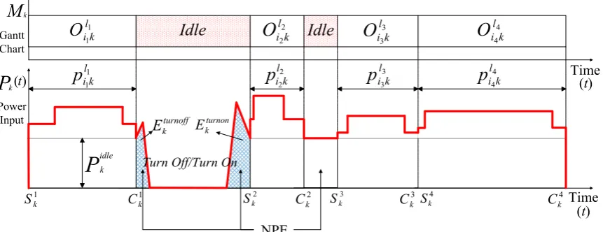
The second part of the ECT model describes the electricity con-sumption. It includes the electricity consumed by the Turn off/Turn on. A power input model for a machine Mkwhen it processes op-eration Oikl assumes that each machine has three constant levels of power consumption: during idle time, when switched into run-time mode and when carrying out the actual cutting operation ( Kor-donowy, 2003). The input power, P tk
( )
, which a machine requires over time is defined as a stepped function represented by the red line inFig. 1. The idle power level of a machine is defined by Pkidle . The overall processing time pikl is defined as the time interval between coolant switching on and off. The objective to reduce the total elec-tricity consumption in the ECT problem can be realised by reducing the total non-processing electricity consumption (NPE). Hence, the objective to minimise the total NPE in a job shop to carry out a given schedule can be expressed as:
⎛ ⎝ ⎜⎜ ⎞ ⎠ ⎟⎟
∑
( ) ( ) =minimise TEM s
2 k m k np 1
whereTEMknp( )s is the NPE of machineMkfor schedules. The NPE is a function of the scheduling plan which needs to be expressed by the sequence of different operations which have been scheduled to be
processed on a machine. Let M′ = {m }∑==∑= γ
k kr ri1 n
l ui
ikl
1 1 denotes thefinite
set of operations to be processed onMk;γik
l is a decision variable such
thatγikl=1if thel-th operation of job Ji is processed on Mk,0 other-wise; Sk
r andCk
r
indicate the start and completion time of operation mk
r
on Mk in schedule s,respectively. In addition to our previous model, here the Turn off/Turn on is applied to idle periods which are long enough. The idle electricity consumption by these periods are replaced by the electricity consumed by turning the machine off and then turning it back on.Ek
turn
is the electricity consumed by Turn off/ Turn on;tkOFFis the time required to turn off machineMkand turn it back on; Bkis the break-even time period of machine Mk for which Turn off/Turn on is economically justifiable instead of running the machine idle,Bk=max(Ek /P ,t )
turn k idle
k OFF
(Mouzon and Yildirim, 2008; Mouzon, 2008).Zk
r
is a decision variable such thatZk=1
r
if a Turn off/ Turn on is applied to the idle period following Ck
r
, 0 otherwise. Consequently, the calculation of the NPE of machine Mk can be ex-pressed as: ⎡ ⎣ ⎢ ⎢ ⎤ ⎦ ⎥ ⎥
( )
( )
∑(
)
∑(
)
∑ ( ) ( ) = × − − − − − × + × + 3TEM s P max C min S C S S C Z E Z
k np
kidle kr kr r k
r kr
r k r
kr kr
k turn
r k r
1
Fig. 1. Let us assume thatOi kl
1 1,O
i k l
2 2,O
i k l
3 3, and O
i k l
4
4 are processed on
machineMk. Expression (3) is used to calculate NPE of machineMk, which is represented by the blue grid area. Firstly the total idle time of Mk is calculated, which equals
(
Ck −Sk)
− ∑r=(
Ck−S)
r k r
4 1
1 4
.
Suppose thatSk2−Ck1>max B t
(
k, kOFF)
, which means it is justifiable to execute a Turn off/Turn on during the idle period betweenOi kl1 1 and
Oi k l
2
2, then Z=1
k1 . Thus, this part of idle time should be
subt-racted from the total idle time, which implies
(
Ck −Sk)
− ∑r=(
Ckr−Skr)
−(
Sk −Ck)
4 1
1
4 2 1
. Then, the aforementioned value is multiplied by the idle power level of machineMkto obtain the total idle electricity consumption. Finally, the electricity con-sumed by the Turn off/Turn on should be summed with the idle electricity consumption to get the value of NPE. In this case, the machine has only been turned off then started again once, so the NPE is calculated as Pkidle×⎣⎡
(
Ck4−Sk1)
− ∑r=1(
Ckr−Skr)
−(
Sk−4 2
⎤ ⎦
)
+Ck Ek turn
1
.
In summary, the multi-objective optimisation problem con-siders minimisation of both TWT (f s1( )) and NPE (f s2( )) which is expressed by Expression (4):
(
)
( ) = ( ) ( ) ∈ ( )
minimiseF s f s f s s1 , 2 S 4
4. A novel multi-objective genetic algorithm for optimisation of energy consumption
The goal of developed GAEJP is to create more opportunities for switching off underutilised resources while maintaining the pro-duction performance. The method for reducing the total non-processing electricity consumption is to integrate fragmented short idle periods into longer idle periods in the operation se-quence on each machine, since this can create opportunities to execute the Turn off/Turn on. The schedule builder used at thefirst step is the semi-active one. The reason for building a semi-active schedule at the initial stage instead of the active one is that in a semi-active schedule normally some operations can be shifted to the left without delaying other operations (Pinedo, 2009;Yamada, 2003). This can create some idle periods which are long enough for executing Turn off/Turn on. The encoding schema and decod-ing procedure of the semi-active schedule builder is explained in the next sub-section.
4.1. Encoding schema and semi-active schedule builder
We adopt the operation-based encoding schema, which is known as“permutation with repetition”(Dahal et al., 2007). Each job’s index number is repeated uitimes (uiis the number of op-erations of Ji). By scanning the permutation from left to right, the l-th occurrence of a job’s index number refers to thel-th operation in the technological sequence of this job. As an illustration, let us follow an example of 33 job shop problem provided byLiu and Wu (2008), whose data are given inTable 1. For example, job J1
requires processing on machinesM1,M2andM3and it takes 2, 2, and 3 time units, respectively.
One of the feasible individuals is[222333111]. Decoded by the active schedule builder (Dahal et al., 2007), the individual is transformed into a feasible schedule as depicted in Fig. 2(a). Comparatively, by employing the semi-active schedule builder (Yamada, 2003), the individual is transformed into a feasible schedule as depicted inFig. 2(b). Normally, the initial semi-active schedule has larger TWT than the active one, but it provides more opportunity for improving the objective values.Fig. 2shows how the improved semi-active schedule outperforms the active one in terms of TWT and the total NPE. The bottom schedule (Fig. 2(c)) is generated based on the middle schedule (Fig. 2(b), semi-active) in the following way: O11
1
is shifted to the left of O21 3
; then O12 2
is moved left to followO32
1
;finallyO13 3
is shifted to the left ofO33 3
. Let us assume that the due date for every job is the 10thtime unit, and
[image:4.595.80.511.62.228.2]that it is justifiable to execute Turn off/Turn on for each machine when the idle period is longer than 3 time units. Thus, it can be seen that the bottom schedule outperforms the other two sche-dules in both the total NPE and TWT. Therefore, the proposed optimisation strategy is to build a semi-active schedule at the in-itial stage, then to improve the schedule by performing left shift and left moving of appropriate operations. The algorithm is de-scribed in detail in the following sub-section.
[image:4.595.300.555.665.745.2]Fig. 1.An example of the Gantt chart for a schedule for machineMkand its corresponding power profile. (For interpretation of the references to colour in thisfigure, the reader is referred to the web version of this article.)
Table 1
An example of a3×3job shop problem.
J1 Oikl
Oik1 Oik2 Oik3 ri di(time unit) wi
4.2. Components of GAEJP
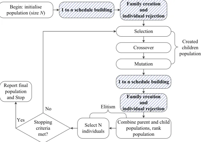
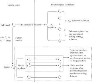
The flowchart of the developed GAEJP is shown in Fig. 3. The structure of the NSGA-II, our algorithm is based on is described by Deb et al. (2002). Two new steps are introduced to address the pre-sented ECT problem which integrates Scheduling and Turn off/Turn on. Thefirst one is labelled“1 to n schedule building”. In this step, each individual in the coding space is decoded into several feasible scheduling plans (solutions) in the solution space, which have dif-ferent idle periods to create opportunities for applying Turn off/Turn on. This expands the solutions pool of a chromosome. The goal of the second step“Family creation and individual rejection”is to select non-dominated solutions from the solutions pool of each individual chromosome and then to further select an elitist solution among them. The operation-based order crossover operator and swap mu-tation operator are adopted fromLiu (2013). The two new steps are explained in detail in the following sub-sections.
4.2.1. One to n schedule building
[image:5.595.139.465.57.288.2]The 1 to n schedule building firstly transforms an individual into a semi-active schedule. All the idle periods within the sche-dule are evaluated tofind those which are sufficiently long to al-low a machine to be turned off and switched back on. Then, the shutdown action is applied to those idle periods, and this gen-erates thefirst feasible solution corresponding to the individual. To improve the schedule’s performance on the TWT objective, two changes to the schedule are introduced: left shift of an operation to the earliest valid time period left to its current position and left move from its current position in the schedule. First, all the op-erations which are allowed to be shifted left in the schedule are ranked according to defined rules. The operation with the highest rank is shifted left to the earliest idle period available for it. After the left shifting, it might be found that some operations can be moved left to further improve the performance on the TWT objective. Then all these permissible left move operations are Fig. 2.Examples of active and semi-active schedules for the ECT problem.
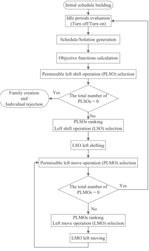
[image:5.595.143.468.503.730.2]selected and ranked. The operation with the highest rank is moved left to its earliest possible starting time. After completing all the aforementioned steps, the algorithm performs iteratively the steps for collecting permissible left move operations, ranking, and left moving until there are no further operations which can be moved left. Then all the idle periods in the generated schedule are eval-uated tofind out those which are justifiable for the Turn off/Turn on. The values of the objective functions are calculated after the Turn off/Turn on is applied. In this way, the second feasible solu-tion corresponding to the considered individual is obtained. The algorithm performs the described steps iteratively until there is no permissible left shift operation in the schedule. The flowchart of 1 tonschedule building step is given inFig. 4, while the details of each step of the algorithm are given in the remainder of the sub-section.
Initial schedule building Employ the semi-active schedule
builder to decode the individual Iptto a semi-active schedule.
Idle periods evaluationEvaluate all the idle periods within the
produced schedule tofind out those for which it is justifiable to apply the Turn off/Turn on and apply it to all of them. After the Turn off/Turn on, thefirst feasible solution which corresponds to individual Iptis obtained, denoted byspt1.
Objective functions calculationCalculate the values of the
ob-jective functions of schedulespt
1.
Permissible left shift operations (PLSO) selection collect all the
operations which are allowed to be shifted left withinspt1. Opera-tion Oik
l
can be defined as a PLSO if there exists at least one idle period before it on machineMk, and the length of the idle period is longer than the required processing time of Oikl.
Permissible left shift operations ranking Rank the selected
PLSOs within schedule spt1. The ranking rules, when applied to operations from different jobs, prioritise the one with a higher ratio of its importance to its due date ( w di/ i). If the values of w di/ i for the two operations are the same, the one with larger weight is prioritised. If wiand diof the two operations are the same, the ranking order is random. For operations from the same job, the one positioned earlier in the technology path is prioritised.
Left shiftingThe operation Oikl which is rankedfirst among all
permissible left shift operations is selected and is shifted to the earliest left-shifting idle period available for it. After the left shift, a new schedule for Iptis obtained, denoted byspt1LS.
Permissible left move operations selectionAfter the left shifting
step has been performed, some operations can be moved left. OperationOikl can be defined as permissible left move operation if there is an idle period just left to it and the completion time ofOikl’s preceding operation is before the starting time of Oikl. All the op-erations which are allowed to be moved left within schedule
spt LS
1
are selected.
Permissible left move operations (LMO) rankingAll the
permis-sible left move operations collected in schedule spt1LS are ranked. The ranking rules are the same as the rules described in permis-sible left shift operations ranking step.
Left movingOperationOikl which is rankedfirst is moved left on
machine Mk to its earliest possible starting time. After the left move, a new schedule for Iptis obtained, denoted byspt
LM
1 . The algorithm goes back to the permissible left move operation selection step and iterates until there is no permissible left moving operation. Once the schedule without any permissible left moving operation has been generated, the idle periods within it are eval-uated tofind out those for which it is justifiable to apply the Turn off/Turn on. Thus, the second feasible solution corresponding to individual Ipt is obtained, denoted by spt
2
. Then the algorithm performs iteratively the steps described above on schedulespt2 until
there is no permissible left shift operation in the schedule. Let us assume that in totalhptfeasible solutions (schedules) which cor-respond to individual Iptare obtained. The solutions assigned to
individualIptare denoted by =
{ }
=Spt spt v
v h
1 pt
.
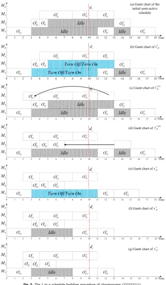
A previously introduced example of 3×3job shop is used to demonstrate the 1 tonschedule building procedure. Suppose the idle power of all machines is 1 power unit and it is justifiable to turn off then turn on a machine if the idle period is longer than 5 time units. To simplify the calculation, supposeEkturn=0,Ekturnis the electricity consumed by Turn Off/Turn On.
Let us consider the individual Ipt=[222333111]. Initially, Ipt is decoded by the semi-active schedule builder to the schedule shown inFig. 5(a). After the Turn Off/Turn On has been applied, the resulting Gantt chart of spt
1
is shown inFig. 5(b). The values of objective functions of spt
1
are
(
27,2)
; the total weighted tardiness is 27 time units, while the non-processing elec-tricity consumption is 2 energy units. There are two permissible left shift operations in spt1, O111 and O321. We select O111 as the left shift operation since J1has larger ratio w d1/ 1(3/10)than J3(1/10). The next step is to perform left shifting step on O111 to obtain
spt;
LS
1 the
[image:6.595.305.552.57.473.2]permissible left move operation in schedulespt LS
1
and that isO12 2
. Left move ofO122 to its earliest possible starting time results in schedule
spt LM
1
. The corresponding Gantt chart is shown inFig. 5(d).
There is just one permissible left move operation in schedulespt1LM, which is O13
3
. It is moved left to its earliest possible starting time. After this move, there is no more available permissible left move operation within the schedule. Since the idle time on machine M3 betweenO13
3
andO13 3
is longer than 5 time units, the Turn Off/Turn On is applied to get the schedule presented inFig. 5(e). This is the second feasible solution for the considered individual, denoted byspt2.
The values of objective functions of spt
2
are
(
21,0)
.Next, the left shift and move continue until no available per-missible left shift operation can be identified. Thus, the 1 to n schedule building process for the given 3×3job shop is com-pleted. Following the above process, Ipt=[222333111]is assigned
four feasible solutions. The Gantt chart ofspt3 andspt4 are shown in Fig. 5(f) and (g), respectively. The values of the four solutions’
[image:7.595.139.468.54.618.2]objective functions are
(
27,2)
,(
21,0)
,(
6,5)
and(
6,5)
. Although spt3 and spt4 have the same values of objective functions, they have different schedules.4.2.2. Family creation and individuals rejection
On the completion of the 1 tonschedule building step, each individual is assigned hpt solutions, hpt≥1. The aim of the step Family creation and individual rejection isfirst to select the non-dominated ones among the hpt solutions corresponding to each individual, and then to preserve one elitist among the selected non-dominated ones. The two steps are described in more details below. The relationship between the coding and solutions space is shown inFig. 6.
4.2.2.1. Family creation. In this step, all solutions in the set Sptin
the solution space associated with individual Ipt in the coding space are compared with each other by using the non-dominated sorting method (Deb et al., 2002), which sorts the solutions into different dominance levels. Only those solutions located in the best level are preserved. The number of solutions corresponding to
Iptis reduced fromhpttoupt, =
{ }
=Spt sptv v u
1 pt
.
EachIptis copiedupt−1times in the population, creating a new
set denoted by =
{ }
=
Ipt Iptv v u
1 pt
.Iptv is decoded into schedulesptv. Hence,
Iptrepresents not a single individual, but a set of individuals, called family. All of the upt individuals in family Ipt are referred to as
“family members”. The members in a family have the same geno-type, i.e. coding but correspond to different phenogeno-type, i.e. sche-dules, and they do non-dominate each other. Before the family creation, there areNindividuals in the populationPtand∑p= h
N pt
1
solutions associated with all individuals, N≤ ∑pN=1hpt.
4.2.2.2. Individual rejections. After the family creation, the
popu-lation size increases from N to N′, where ′ = ∑
=
N pN 1upt. Thus, the aim of the individuals rejection is to preserve the elitist in each family, keep the diversity of the population, and reduce the po-pulation size fromN′back toN. Two types of individual rejections
are defined to decide on which family members to keep for the next generation: individual rejections based on non-dominated sorting of the whole population which is followed by individual rejections in a family based on crowding distance.
Individuals rejection in the population based on non-dominated
sorting. The non-dominated sorting is performed on all N′
solu-tions in populationPt. As a result, the solutions which correspond to family members are sorted into different levels. Thus, within a family Ipt, only members whose corresponding solutions are lo-cated in the lowest level are preserved, others are abandoned. For example, let us assume that there are three members in the family
Ipt, Ipt1, Ipt2 and Ipt3, and that their corresponding solutions
(sche-dules) arespt1,spt2 and spt3. Let us further assume that based on the
non-dominated sorting,spt
1
is located in level 2,spt
2
in level 3 andspt
3
in level 4. In that case, onlyIpt1 is preserved, while bothIpt2 and Ipt3 are abandoned. By completing this process, all the solutions of the members in a specific family are located in the same level, and the population size ofPtis now equal to N′′, N′ ≥N′′≥N. Some mem-bers still need to be rejected from each family to reduce the po-pulation size back toN.
[image:8.595.132.456.447.734.2]Individuals rejection in a family based on crowding distance. According toDeb et al. (2002), the crowding distance is an im-portant indicator which evaluates the ability of an individual to contribute to the diversity of the population. In this step, the preserved family members whose corresponding solutions are located in the same non-dominated front are ranked by their crowding distance value. The one with the largest crowding dis-tance is made elitist.Hence, the boundary solutions of each non-dominated front are kept since they have an infinite value of crowding distance (Deb et al., 2002). In order to address the pre-sence of families in our algorithm we propose a modified defi ni-tion of boundary soluni-tions and a modified neighbours search to choose solutions to be used in the crowding distance calculation.
The boundary solutions have to belong to different families. They are defined in the following way. In each front Fi, two boundary solutions are found with minimum and maximum value of each objective (see Fig. 7, where different shapes represent solutions from different families, the x-axis representsNPE, while y-axis represents TWT). The solutions with minimum and max-imum value ofNPEare boundary solutions which are denoted by BSFmini andBSFmaxi , respectively. There are two possible relationships between two boundary solutions, which determine which one among two of them will be kept.
(1) The individuals that correspond toBSFmini andBSFmaxi belong to different families. Then both of them are preserved.
(2) The individuals which correspond toBSF min
i andBSF max
i belong to the same family. Then one of them is randomly chosen and preserved. Thus, another boundary solution needs to be found such that the individual corresponding to it belongs to a fa-mily different from the preserved one. Let us suppose that BSFmini is preserved, then the newBSFmaxi needs to be found. The
first solution in the list sorted by NPE in descending order whose corresponding individual belongs to a different family thanBSFmini one is defined as the newBSFmaxi . An example of the search process is depicted in Fig. 7. Analogue procedure applies if BSFmaxi is preserved and newBSF
min
i has to be found.
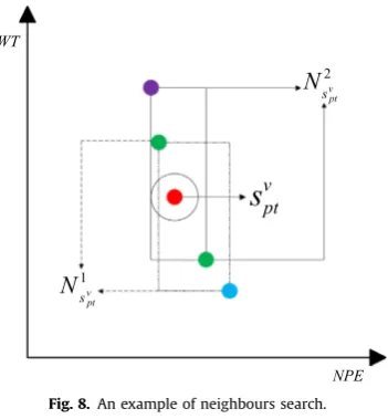
The solutions to be used in the calculation of crowding distance of each solution are chosen in the following way. The neighbours of solutionsptv are the“closest”solutions in terms of the values of TWT or NPE whose corresponding individuals belong to different families. Their families have also to be different from the family of the corre-sponding individualIptv. Normally, there are two groups of neighbours for each solution. Thefirst group, denoted by N
s
1
ptv is obtained by
takingfirst the left and then the right neighbour ofsptv, which satisfy the family conditions, while the second group, denoted by N
s
2 ptv is obtained takingfirst the right neighbour and then the left. This is illustrated inFig. 8. The crowding distance of a solution is the max-imum between the crowding distance calculated by using N
s
1 ptv and
Ns2
ptv. Each solution has at least one group of neighbours due to the existence of the preserved boundary solutions.
Based on above, the two individuals from different families corresponding to the boundary solutions are preserved. In each of the remaining families, the individual with the largest crowding distance is preserved, while others are rejected. Completing this step, the population size is decreased toN.
A simplified example with the population size of 2 (N=2) is shown inFig. 9to show the family creation and individual rejec-tion process.
5. Experimental results
The effectiveness of the developed GAEJP is validated based on comparison experiments. The solutions of GAEJP are compared with the solutions obtained by the traditional single objective scheduling methods and NSGA-II. Three job shop instances based on the F&T 10×10 (Fisher and Thompson, 1963), Lawrence
×
15 10and 20×10(Lawrence, 1984) instances are modified to incorporate electrical consumption profiles for the machine tools. The due date for each job is defined by the TWK due
date assignment method (Sabuncuoglu and Bayiz, 1999),
= × ∑= ∑= = ⋯
di f k p ,i 1, 2, ,n
m l u
ik l
1 i1 where f is the tardiness factor.
The following values of f are set:1.5,1.6,1.7,1.8and 1.9. These values have the trend of less tight due date. For instance, f=1.5, represents a tight due date case which corresponds to 50% of tardy jobs. The weight of each job is randomly allocated. The time unit is a minute. Assuming that all the machine tools are automated ones, the idle power level and electricity consumed by Turn off/Turn on of each machine are generated based on the research works fo-cused on the characterisation of machine tools’ electricity con-sumption, such asDahmus (2007),Drake et al. (2006), andLv et al. (2016). They provided us with reasonably defined ranges within which required values are generated randomly. A complete list of electrical characteristics data of machines used in the experiments can be found in Appendix I inLiu (2013).
To demonstrate the effectiveness of GAEJP in solving the ECT problem, the following comparison experiment is carried out. The classical job shop scheduling problem with the single objective to minimise TWT serves as the benchmark to represent the tra-ditional approach to machine scheduling without the electricity saving consideration. Shifting Bottleneck Heuristic (SBH) and Local Search Heuristic (LSH) provided by the software LEKIN (Pinedo, 2009) are used to produce solutions. The solutions with minimum TWT are adopted. In each generated schedule, the total NPE value is calculated without using it as the objective function. Perfor-mance of SBH and LSH under different due date conditions are shown inTables 2–4. In the next experiments, the goal is to prove superiority of GAEJP to NSGA-II in solving the ECT problem.
[image:9.595.77.258.55.217.2]The parameter values used in the GAEJP obtained by tuning, are as follows: population size N=150; crossover probability pc=1.0; mutation probabilitypm=0.4; generationt=8000. The algorithm is Fig. 7.An example of boundary solutions.
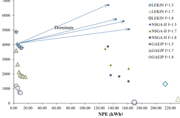
[image:9.595.352.528.56.246.2]run 5 times. Considering the possibility of accelerating machine wear by frequent turn off and turn on actions, they are applied only when the idle time on the machine is longer than30minutes. Part of the comparison among solutions of GAEJP, NSGA-II and LEKIN are shown inFigs. 10–12. The trend of results for remaining values of f is similar.
In Figs. 10–12, the hollow points represent the solutions ob-tained by LEKIN which had been shown inTables 2–4, the solid
points and the points with a pattern are produced by NSGA-II, and GAEJP, respectively. GAEJP achieves a considerable total NPE re-duction. The NPE improvements are shown inTables 5and6. Take the F&T 10×10job shop as an example, when f=1.5and the machines are turned off when the idle time is longer than30min, the minimum and maximum values of total NPE obtained by GAEJP are 3.5 kWh and 6.0 kWh respectively, which means that it achieved from 96.7% to 98.1% improvement in the total NPE con-sumption compared to the values obtained by LEKIN. With the same f value, the improvement in the total NPE compared to NSGA-II is from 90.3% to 98.0%. The TWT deterioration of GAEJP results (compared to the LEKIN results) in weighted minute for each job shop instance under different tardiness conditions are shown inTables 7and8. By considering the performance in both the total NPE and TWT objectives, it can be noticed that scheduling plans delivered by GAEJP always have much smaller NPE con-sumption than scheduling plans delivered by NSGA-II if they have similar values of TWT. For instance, in the F&T10×10job shop instance, whenf=1.6, one of the boundary solutions delivered by GAEJP is
(
1118minutes,12.2kWh)
; comparatively, the solutionob-tained by NSGA-II with the closest value of TWT is
(
1136minutes,170kWh)
, which means the most of the solutionsgenerated by NSGA-II are dominated by solutions delivered by GAEJP. This can also be observed in the givenfigures.
[image:10.595.76.507.59.325.2]Additional experiments have been carried out to investigate the effectiveness of GAEJP in reducing the NPE when different values of the minimum idle period allowing machine to be turn off are applied, namely using 20, 40, 50 and 60min. We present the minimum improvement in NPE achieved across all runs of the algorithm (Tables 5 and 6). These solutions belonging to Pareto fronts, have the minimum compromise in TWT, i.e. they achieve at the same time minimum increase in TWT (Tables 7and8). Based on the experiment results, it can be concluded that GAEJP is ef-fective in reducing the NPE at different levels of idle times on the machines allowing them to be turned off. Although in many cases smaller values of the minimum idle period allowing a machine to be turned off lead to larger improvements in NPE, one cannot Fig 9.An example of the family creation and individuals rejection.
Table 2
The performance of SBH and LSH on the F&T10×10job shop by LEKIN.
Tardiness factor (f) TWT (weighted min) Total NPE (kW h) Heuristic
1.5 309 181 SBH
1.6 127 181 SBH
1.7 25 169.7 LSH
[image:10.595.33.285.378.438.2]1.8 0 169.7 LSH
Table 3
The performance of SBH and LSH on the Lawrence15×10job shop by LEKIN.
Tardiness factor (f) TWT (weighted min) Total NPE (kW h) Heuristic
1.5 1321 212.8 LSH
1.6 694 207.7 LSH
1.7 293 230.7 LSH
1.8 53 169.3 LSH
1.9 0 200.0 LSH
Table 4
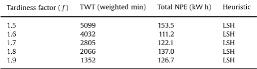
The performance of SBH and LSH on the Lawrence20×10job shop by LEKIN.
Tardiness factor (f) TWT (weighted min) Total NPE (kW h) Heuristic
1.5 5099 153.5 LSH
1.6 4032 111.2 LSH
1.7 2805 122.1 LSH
1.8 2066 137.0 LSH
[image:10.595.32.285.476.544.2] [image:10.595.32.284.582.650.2]Fig. 10.Performance comparison of GAEJP, NSGA-II and LEKIN (F&T10×10job shop).
Fig. 11.Performance comparison of GAEJP, NSGA-II and LEKIN (Lawrence15×10job shop).
[image:11.595.143.463.542.732.2]conclude that it holds all the time. For instance, the largest mini-mum NPE improvement compared to the LEKIN results for E-Lawrence20×10,f=1. 7, was achieved when the minimum idle period for turning of the machine was 30 min. On the other hand, the compromise of TWT varies considerably when different values of the minimum idle period allowing machine to be turned off are applied. For instance, in the E-Lawrence15×10job shop, f=1. 9, the increase in TWT is only10when40min is used as the lower boundary to turn off the machines, compared to the LEKIN result, while the improvement in NPE is 75.5%. This is the best value of TWT across all five evaluated lower boundaries of idle periods. Thus, it can be concluded that for a specific job shop, it is worthy
investigating which value of the minimum idle period allowing the machines to be turned off will result in the good trade-off between TWT and NPE. From the application perspective, this can provide more options for the decision maker. For example, for the E-Lawrence 15×10 job shop, f=1. 9, when 40min is used to apply the turn off, the solution with 75.5% improvement in NPE and only10increase in TWT might be more preferable than the solution with 98.3% improvement in NPE and647increase in TWT (obtained by using30min idle period to apply the turn off).
It can be observed that GAEJP combined with Turn off/Turn on is more effective in reducing the total NPE than NSGA-II, without compromising TWT too much. For Lawrence15×10and20×10
[image:12.595.33.558.79.258.2]job shop, all solutions obtained by NSGA-II are dominated by at least one solution obtained by GAEJP, as shown inFigs. 11and12. For the F&T 10×10instance, some of the NSGA-II solutions are not dominated by any GAEJP solutions. For this instance, Pareto fronts generated by two algorithms are combined together to form new Pareto fronts, and only non-dominated solutions are pre-served. It can be noticed fromFig. 10that solutions obtained by the GAEJP take a larger proportion of the total number of solutions in Table 5
The total NPE improvement in percentage for F&T10×10and Lawrence15×10instance.
Comparison of GAEJP and LEKIN E-F&T10×10 E-Lawrence15×10
f¼1.5 f¼1.6 f¼1.7 f¼1.8 f¼1.5 f¼1.6 f¼1.7 f¼1.8 f¼1.9
NPE Improvement 20 min 95.6% 96.8% 97.2% 96.9% 96.1% 88.9% 97.3% 95.7% 96.3%
NPE Improvement 30 min 96.7% 93.2% 93.9% 95.0% 94.8% 94.5% 93.0% 94.3% 96.0%
max 98.1% 98.1% 97.4% 98.6% 98.4% 98.0% 98.6% 98.0% 98.3%
NPE Improvement 40 min 93.5% 92.1% 96.3% 90.7% 91.9% 93.1% 92.5% 92.3% 95.1%
NPE Improvement 50 min 94.9% 91.1% 90.8% 89.9% 94.1% 88.2% 94.5% 91.7% 96.3%
NPE Improvement 60 min 89.2% 94.5% 88.3% 91.9% 89.2% 88.4% 91.7% 82.8% 90.3%
Comparison of GAEJP and NSGA-II E-F&T10×10 E-Lawrence15×10
f¼1.5 f¼1.6 f¼1.7 f¼1.8 f¼1.5 f¼1.6 f¼1.7 f¼1.8 f¼1.9
NPE Improvement 20 min 87.2% 90.4% 92.6% 91.4% 93.7% 80.7% 95.2% 94.5% 94.1%
NPE Improvement 30 min 90.3% 80.1% 83.9% 86.3% 91.7% 90.4% 87.4% 92.8% 93.7%
max 98.0% 98.0% 97.1% 98.3% 97.8% 97.4% 97.9% 97.9% 98.1%
NPE Improvement 40 min 80.9% 76.7% 90.3% 74.4% 87.0% 88.0% 86.6% 90.2% 92.3%
NPE Improvement 50 min 85.0% 73.8% 75.7% 72.2% 90.5% 79.4% 90.1% 89.4% 94.2%
[image:12.595.34.283.294.472.2]NPE Improvement 60 min 68.2% 83.8% 69.1% 77.6% 82.7% 79.8% 85.2% 77.9% 84.8%
Table 6
The total NPE improvement in percentage for Lawrence20×10instance.
Comparison of GAEJP and LEKIN E-Lawrence20×10
f¼1.5 f¼1.6 f¼1.7 f¼1.8 f¼1.9
NPE Improvement 20 min 92.4% 86.5% 93.8% 94.5% 94.0% NPE Improvement 30 min 90.1% 93.3% 94.1% 91.5% 90.1% max 97.1% 96.9% 97.1% 96.7% 96.5% NPE Improvement 40 min 87.3% 81.5% 90.3% 85.8% 87.2% NPE Improvement 50 min 80.3% 69.0% 77.4% 87.7% 81.8% NPE Improvement 60 min 77.8% 76.8% 79.9% 75.7% 81.7%
Comparison of GAEJP and NSGA-II E-Lawrence20×10
f¼1.5 f¼1.6 f¼1.7 f¼1.8 f¼1.9 NPE Improvement 20 min 81.5% 74.0% 87.6% 88.2% 88.5% NPE Improvement 30 min 75.9% 87.0% 88.3% 81.9% 81.1% max 95.0% 95.9% 95.6% 94.1% 95.5% NPE Improvement 40 min 69.1% 64.3% 80.7% 69.8% 75.5% NPE Improvement 50 min 52.1% 40.2% 55.2% 73.9% 65.0% NPE Improvement 60 min 46.2% 55.4% 60.1% 48.2% 64.9%
Table 7
The TWT increase in weighted minutes for F&T10×10and Lawrence15×10.
Comparison of GAEJP and LEKIN E-F&T10×10 E-Lawrence15×10
f¼1.5 f¼1.6 f¼1.7 f¼1.8 f¼1.5 f¼1.6 f¼1.7 f¼1.8 f¼1.9
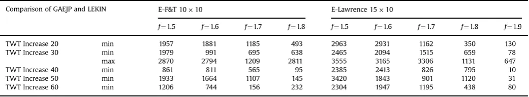
TWT Increase 20 min 1957 1881 1185 493 2963 2931 1162 350 130
TWT Increase 30 min 1979 991 695 638 2465 2094 1515 659 78
max 2870 2794 1209 2811 3555 3165 3306 1131 647
TWT Increase 40 min 861 811 565 95 2385 2413 826 795 10
TWT Increase 50 min 1933 1664 1107 145 3420 1843 901 1120 31
[image:12.595.303.554.296.390.2]TWT Increase 60 min 1206 744 156 232 2304 1947 1195 438 80
Table 8
The TWT increase in weighted minutes for Lawrence20×10.
Comparison of GAEJP and LEKIN E-Lawrence20×10
f¼1.5 f¼1.6 f¼1.7 f¼1.8 f¼1.9
[image:12.595.33.554.650.746.2]the new Pareto fronts, which means GAEJP can provide more op-tions to the production manager.
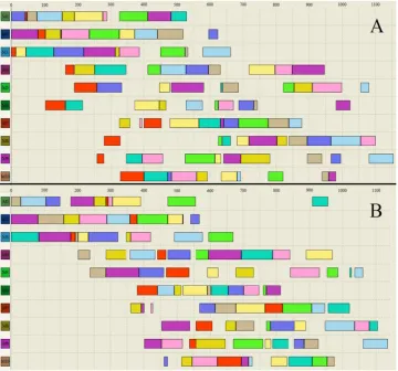
The upper part A and bottom part B ofFig. 13show the Gantt charts of optimal schedules produced by GAEJP and NSGA-II re-spectively for E-F&T10×10job shop instance when f=1.5. It can be observed that the schedule produced by GAEJP has a smaller total amount of idle periods on all machines (31 idles periods on the GAEJP schedule versus 37 idle periods on the NSGA-II sche-dule), and in general the lengths of those idle periods are longer. This means when the varieties of jobs’ components and their amounts are increasing, it is easier to place the new operations in the existing idle periods in scheduling plans produced by GAEJP. From above, the scheduling plans produced by GAEJP might be more preferable for managers when considering the real life job shop manufacturing system. An interesting question is whether the Turn off/Turn on applied to the optimisation result of NSGA-II may lead to a better result than that produced by GAEJP. However, in the case presented in Fig. 13, the original objective function values of scheduling plans produced by GAEJP and NSGA-II are
(
2288 min,6.0 kW h)
and(
3595 min,170 kW h)
, respectively. When the Turn off/Turn on is applied to the bottom scheduling plan, the objective function values become(
3595 min,14.5 kW h)
. Therefore, the solution delivered by GAEJP is still preferable for the produc-tion manager. A more thorough investigaproduc-tion of the effects of applying Turn off/Turn on to the optimisation results of NSGA-II will be investigated in the future research work.6. Conclusions and future work
Reducing electricity consumption as well as keeping good performance in classical scheduling objectives gains more and
[image:13.595.123.484.58.394.2]investigated how to set a favourable value of the minimum idle period allowing the machines to be turned off for a specific job shop.
Acknowledgement
The authors acknowledge the support from the EPSRC Centre for Innovative Manufacturing in Intelligent Automation in under-taking this research work under grant reference number EP/ IO33467/1.
References
Artigues, C., Lopez, P., Haït, A., 2013. The energy scheduling problem: Industrial case-study and constraint propagation techniques. Int. J. Prod. Econ. 143 (1), 13–23.
Bruzzone, A.A.G., Anghinolfi, D., Paolucci, M., Tonelli, F., 2012. Energy-aware sche-duling for improving manufacturing process sustainability: a mathematical model forflexibleflow shops. CIRP Ann. Manuf. Technol. 61, 459–462. Dahal, K.P., Tan, K.c., Cowling, P., 2007. Evolutionary Scheduling,Series: Studies in
Computational Intelligence. Vol. 49. Springer.
Dahmus, J.B., 2007. Applications of Industrial Ecology Manufacturing, Recycling, and Efficiency. Massachusetts Institute of Technology.
Dai, M., Tang, D.B., Xu, Y.C., Li, W.D., 2014. Energy-aware integrated process plan-ning and scheduling for job shops. Proc. Inst. Mech. Eng. Part B: J. Eng. Manuf. 0954405414553069
Deb, K., Pratap, A., Agarwal, S., Meyarivan, T., 2002. A Fast and Elitist Multiobjective Genetic Algorithm NSGA-II. IEEE Trans. Evolut. Comput.6, 182–197. Drake, R., Yildirim, M. B., Twomey, J., Whitman, L., Ahmad, J., & Lodhia, P., 2006.
Data collection framework on energy consumption in manufacturing. In: Pro-ceedings of the Industrial Engineering Research Conference, Institute of In-dustrial Engineers Annual Meeting. Orlando, FL.
Du, B., Chen, H.P., Huang, G.Q., Yang, H.D., 2011. Preference vector ant colony system for minimising make-span and energy consumption in a hybridflow shop. In: Wang, L., Ng, A.H.C, Deb, K. (Eds.), Multi-objective Evolutionary Optimisation for Product Design and Manufacturing. Springer, pp. 279–304.
Fang, K., Uhan, N., Zhao, F., Sutherl, J.W., 2011. A new shop scheduling approach in support of sustainable manufacturing. In: Hesselbach, J., Herrmann, C. (Eds.), Glocalised Solutions for Sustainability in Manufacturing. Springer, pp. 305–310. Fisher, H., Thompson, G.L., 1963. Probabilistic learning combinations of local
job-shop scheduling rules. In: Thompson, J.F.M. a G.L. (Ed.), Industrial Scheduling. Prentice-Hall, NJ, Englewood Cliffs, pp. 225–251.
Gahm, C., Denz, F., Dirr, M., Tuma, A., 2016. Energy-efficient scheduling in manu-facturing companies: a review and research framework. Eur. J. Oper. Res. 248 (3), 744–757.
Gutowski, T., Murphy, C., Allen, D., Bauer, D., Bras, B., Piwonka, T., Sheng, P., Su-therland, J., Thurston, D., Wolff, E., 2005. Environmentally benign manu-facturing: observations from Japan, Europe and the United States. J. Clean. Prod.
13, 1–17.
He, Y., Liu, B., Zhang, X., Gao, H., Liu, X., 2012. A modeling method of task-oriented energy consumption for machining manufacturing system. J. Clean. Prod.23, 167–174.
Kilian, L., 2008. The economic effects of energy price shocks. J. Econ. Lit.46,
871–909.
Kordonowy, D., 2003. A power assessment of machining tools. Bachelor thesis. Massachusetts Institute of Technology.
Lawrence, S., Resource Constrained Project Scheduling: An Experimental In-vestigation of Heuristic Scheduling Techniques (Supplement), 1984, Pittsburgh: Graduate School of Industrial Administration, Carnegie Mellon University. Liu, M., Wu, C., 2008. Intelligent Optimization Scheduling Algorithms for
Manu-facturing Process and Their Applications. National Defense Industry Press. Liu, Y., 2013. Multi-objective Optimisation Methods for Minimising Total Weighted
Tardiness, Electricity Consumption and Electricity Cost in Job shops Trough Scheduling. PhD thesis, University of Nottingham, United Kingdom. Liu, Y., Dong, H.B., Lohse, N., Petrovic, S., 2015. Reducing environmental impact of
production during a rolling blackout policy–a multi-objective schedule opti-misation approach. J. Clean. Prod. 102, 418–427.
Liu, Y., Dong, H., Lohse, N., Petrovic, S., Gindy, N., 2014. An investigation into minimising total energy consumption and total weighted tardiness in job shops. J. Clean. Prod.65, 87–96.
Luo, H., Du, B., Huang, G.Q., Chen, H., Li, X., 2013. Hybridflow shop scheduling considering machine electricity consumption cost. Int. J. Prod. Econ. 146 (2), 423–439.
Lv, J.X., Tang, R.Z., Jia, S., Liu, Y., 2016. Experimental study on energy consumption of computer numerical control machine tools. J. Clean. Prod. 112, 3864–3874. Mansouri, S.A., Aktas, E., Besikci, U., 2016. Green scheduling of a two-machine
flowshop: trade-off between makespan and energy consumption. Eur. J. Oper. Res. 248 (3), 772–788.
Mouzon, G., 2008. Operational methods and models for minimisation of energy consumption in a manufacturing environment. Wichita State University. Mouzon, G., Yildirim, M.B., 2008. A framework to minimize total energy
con-sumption and total tardiness on a single machine. Int. J. Sustain. Eng. 1 (2), 105–116.
Mouzon, G., Yildirim, M.B., Twomey, J., 2007. Operational methods for minimiza-tion of energy consumpminimiza-tion of manufacturing equipment. Int. J. Prod. Res.45, 4247–4271.
Pinedo, M.L., 2009. Planning and Scheduling in Manufacturing and Services. Springer.
Pinedo, M.L., 2012. Scheduling: Theory, Algorithms, and Systems. Springer. Sabuncuoglu, I., Bayiz, M., 1999. Job shop scheduling with beam search. Eur. J. Oper.
Res.118, 390–412.
Subaï, C., Baptiste, P., Niel, E., 2006. Scheduling issues for environmentally re-sponsible manufacturing: the case of hoist scheduling in an electroplating line. Int. J. Prod. Econ.99, 74–87.
Tang, L.X., Wang, G.S., 2008. Decision support system for the batching problems of steelmaking and continuous-casting production. Omega36(6), 976–991. Tang, L.X., Liu, J.Y., Rong, A.Y., Yang, Z.H., 2000. A multiple traveling salesman
problem model for hot rolling scheduling in Shanghai Baoshan Iron & Steel Complex. Eur. J. Oper. Res.124(2), 267–282.
Wang, J., Li, J., Huang, N., 2011. Optimal vehicle batching and sequencing to reduce energy consumption and atmospheric emissions in automotive paint shops. Int. J. Sustain. Manuf.2, 141–160.
Yamada, T., 2003. Studies on Metaheuristics for Job Shop and Flow Shop Scheduling Problems. Kyoto University.
Zanoni, S., Bettoni, L., Glock, C.H., 2014. Energy implications in a two-stage pro-duction system with controllable propro-duction rates. Int. J. Prod. Econ. 149, 164–171.