LOCAL MINIMUM PROBLEM
Jonathan Peter Lewis
A Thesis Submitted for the Degree of PhD
at the
University of St Andrews
2002
Full metadata for this item is available in
St Andrews Research Repository
at:
http://research-repository.st-andrews.ac.uk/
Please use this identifier to cite or link to this item:
http://hdl.handle.net/10023/14985
Using Subgoal Chaining to Address
The Local Minimum Problem
A thesis submitted to the
UNIVERSITY OF ST ANDREWS
for the degree of
DOCTOR OF PHILOSOPHY
by
Jonathan Peter Lewis
School of Computer Sciences
University of St Andrews
All rights reserved
INFORMATION TO ALL USERS
The quality of this reproduction is dependent upon the quality of the copy submitted.
In the unlikely event that the author did not send a com plete manuscript and there are missing pages, these will be noted. Also, if material had to be removed,
a note will indicate the deletion.
uest
ProQuest 10170993
Published by ProQuest LLO (2017). Copyright of the Dissertation is held by the Author.
All rights reserved.
This work is protected against unauthorized copying under Title 17, United States C ode Microform Edition © ProQuest LLO.
ProQuest LLO.
789 East Eisenhower Parkway P.Q. Box 1346
I, Jonathan Peter Lewis, hereby certify that this thesis, which is approximately 44,000
words in length, has been written by me, that it is the record of work carried out by me, and
that it has not been submitted in any previous application for a higher degree.
date a__^ ^ __________ signature o f candidate
I was admitted as a research student in November 1997 and as a candidate for the degree
of Doctor of Philosophy in November 1998; the higher study for which this is a record was
carried out in the University of St Andrews between 1997 and 2001.
date Aé—ï A i ^ signature of candidate
I hereby certify that the candidate has fulfilled the conditions of the Resolution and Regu
lations appropriate for the degree of Doctor of Philosophy in the University of St Andrews
and that the candidate is qualified to submit this thesis in application for that degree.
In submitting this thesis to the University of St Andrews I understand that I am giving
permission for it to be made available for use in accordance with the regulations of the
University Library for the time being in force, subject to any copyright vested in the work
not being affected thereby. I also understand that the title and abstract will be published,
and that a copy of the work may be made and supplied to any bona fide library or research
worker.
-A common problem in the area of non-linear function optimisation is that of not being able
to guarantee finding the global optimum of the function in a feasible time especially when
local optima exist. This problem applies to various areas of heuristic search. One of these
areas concerns standard training techniques for feedforward neural networks. The element
of heuristic search consists of attempting to find a neural weight state coiTesponding to the
lowest training error. This problem may be termed the local minimum problem.
The local minimum problem is addressed for feedforward neural networks. This is done by
first establishing the conditions under which local minimum interference for the training
process is to be expected. A target based approach to subgoal chaining in supervised leain-
ing is then investigated. This is a method to improve travel for neural networks by directing
it more precisely through local subgoals than may be achieved through a more distant goal.
It is shown however that linear subgoal chains aie not sufficient to overcome the local min
imum problem. Two novel training techniques are presented which use non-linear subgoal
chains and are examined for their capability to address the local minimum problem.
It is found that attempting to target a neural network to do something it cannot may lead to
suboptimal training. It is also found that targeting a network to do something it is capable
of generally leads to successful training. A novel system is presented which is designed to
create optimal realisable targets for unrealisable goals. This allows neural networks to sub
sequently achieve the optimal weight state through a sufficiently powerful training method
such as subgoal chaining. The results are shown to be consistent with the theoretical ex
Acknowledgements
The most sincere thanks to Mike Weir, without whose constant encouragement and tireless
supervisory commitment this thesis and the work it entailed would not have been possible.
My deepest gratitude goes to my parents, whose moral and financial support over the years
has enabled me to complete my work.
I would also like to thank Brian, Helen and Joy, from the School of Computer Science.
Last, but certainly not least, I would like to thank all my friends for their unwaivering
support.
1 Goal Directed Learning for Neural Networks
1.1 Neural Networks
1.1.1 The Brain as a Neural C om puter... 1
1.1.2 Feedforward Neural N etw orks... 4
1.1.3 Learning for Neural N etw orks... 6
1.2 The Local Minimum Problem ... 8
1.3 Goal Directed T rain in g ... 11
1.4 Thesis Structure... 14
1.5 N otation... 16
1.5.1 Mathematical N otation... 16
2 Common Neural Training Techniques 20
2.1 Back-propagation... 21
2.2 Conjugate Gradient D e s c e n t...29
2.3 Levenberg-Marquardt... 35
2.4 Simulated A n n ealin g ... 38
2.5 C o n clu sio n ...41
3 Goal Directed Behaviour and Symbolic AI 43 3.1 Common Seai'ch Techniques in Symbolic A I ... 43
3.2 The Use and Selection of Subgoals in Symbolic A I ... 63
3.3 Conclusions... 68
4 Linear Subgoal Chaining for Neural Networks 69 4.1 Tangent H yperplanes...69
4.2 Extending TH’s Subgoal Acceptance C rite ria ... 81
4.3 Linear Subgoal Chaining Issues ... 88
4.4 Expanded Range Approxim ation...92
5 Local Minima and Unrealisable Regions 100
ii
5.2 Unrealisable R eg io n s...113
5.3 Experiments with E R A ...127
6 Non-linear Subgoal Chaining 135 6.1 Non-linear Subgoal Chaining with Cheat C hains...137
6.1.1 Experimental Results with Cheat Chains...139
6.2 The Z IP -m o d e l...142
6.3 Realisable and Progressive D ire c tio n s...147
6.4 Experimental R e su lts... 150
6.5 S u m m a ry ...152
7 Hyperspherical TH 153 7.1 The Need for B etter Directi on ... 153
7.2 Hyperspherical TH: The M eth o d ...155
7.2.1 Direction Angle Hyperplanes ...156
7.2.2 Hyperplanes in Delta Weight S p a c e ... 160
7.3 Good Direction Not E n o u g h ...163
8 The Global Positioning System 167
8.1 Realisable Manifolds in Excitation S p a c e...170
8.2 Realisable Curved Manifolds in Output S p a c e ...174
8.3 A Semi-linear Approximation ... 177
8.4 Realisable Hyper-surfaces in Output Space...183
8.5 Finding Minimum Output S ta te s ... 188
8.6 The GPS A lgorithm ...193
8.6.1 Stage 1 ... 193
8.6.2 Stage 2 ... 194
8.6.3 Complexity I s s u e s ...195
8.7 Experiments and Discussion of R esults...196
8.7.1 Artificial Examples in 3 - D ... 196
8.7.2 Neural Training Problem 1 ... 199
8.7.3 Neural Training Problem 2 ...205
9 Overall Conclusions and Further Work 210 9.1 Overall Conclusions...210
9.2.1 Extending G P S ...214
9.2.2 GPS Applied to Function M inim isation... 216
9.2.3 The Use of GPS with regard to Generalisation... 217
List of Figures 219
List of Tables 222
Chapter 1
Goal Directed Learning for Neural
Networks
1.1 Neural Networks
1.1.1 The Brain as a Neural Computer
When looking at the brain as a computing unit we can see that in many areas it is more
powerful than some of today’s most sophisticated computer systems, especially in areas
concerning vision, speech, motor control and facial recognition, i.e. tasks which would be
considered to be easy for humans to perform. The brain has the ability to form generalisa
tions and characterise objects or circumstances that it has not been subjected to before, to a
in the sense that if parts of it are slightly damaged it can still function and in some cases will
adapt. Flexibility, fault tolerance and generalisation ability coupled with a highly parallel
design may be seen as features which are desirable when a system is required to function
in the real world. This realisation can be seen as the main motivation to investigate ways
of making the architecture of computers more similar to that of our brain.
A neural network can be seen as a group of interconnected simple units in which the struc
ture and type of connections between the units define the computational capability of the
network.
One of the early models which is a basis for most neural networks was suggested by neuro
physiologist Warren McCulloch and logician Walter Pitts in 1943 and described the brain
as consisting of many interconnected neurons. Their model has these neurons sending sim
ple messages to each other which are excitatory or inhibitory pulses and has the neurons
updating their excitations on the basis of these messages. They subsequently proposed a
model for a neural network consisting of an array of variable resistors on connection lines
between summing amplifiers to mimic the way in which neurons operate in the brain.
In 1949 Donald Hebb suggested that a group of neurons could reverberate in different pat
terns which could correspond to the brain remembering different experiences. Hebb also
speculated about synaptic modification by which learning could possibly be achieved. In
1962 Frank Rosenblatt coined the expression perceptron with which he refeired to a learn
ing image recognising unit based on McCulloch and Pitts’ model combined with some
Ch a pter 1. Goal Dir ec ted Le a r n in g fo r Neu ra l Netw o r k s 3
ferent context, i.e. omitting the feature detectors. With this adjustment the term perceptron
has survived and denotes a simple unit which is capable of learning and may be a part of
an arrangement of many such units, i.e. a neural network. He also produced a convergence
theorem for perceptrons that guarantees them converging to a solution in finite time if one
exists, by using a learning rule which can either increase or reduce the connective strengths.
In their book Perceptrons Minsky and Papert describe the class of problems which may be
solved by perceptrons as very restricted, i.e. to those only involving linear mappings. This
limitation on the use of perceptrons may be seen as a reason for a decline in research taking
place in that area.
A way to overcome the limitation of the perceptron was found by extending its aichitecture
to allow multiple layers of neurons and finding a learning rule to train them. Today this
type of network is generally called a multi-layer feedforwairi network and the learning rule
used to train it is now called eiTor propagation, back-propagation or generalised delta rule
and was popularised in 1986 by Rummelhart, Hinton and Williams in [RM86].
The mapping ability of multi-layer feedforward networks was shown to be superior to that
of the perceptron. In paiticular, the class of solvable problems broadens to include non
linear as well as linear mappings and the availability of back-propagation as a learning rule
1.1.2 Feedforward Neural Networks
There are many different types of artificial neural network (ANN), but I will be merely
concentrating my studies on so-called feedforward neural networks. This type of network
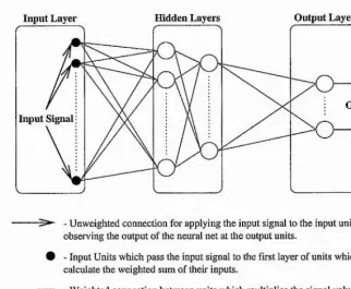
can be seen to describe an arrangement of units in different layers such as input layer, output layer and intermediate hidden layers. Figure 1.1 is a stylised view of a feedforward neural
network. In a fully connected network each unit in one layer is connected to all units in
adjacent layers via weighted connections. If the network is strictly layered then connections
are only between units in adjacent layers. The weight on a connection modifies the strength
of a signal value being passed along the connection by multiplying the signal value by the
numerical value of the weight.
In general an input signal consisting of a numerical value for each unit in the input layer
is applied. Each unit in the adjacent layer of units calculates the weighted sum of the
incoming signal values which is termed its excitation. The units’ excitation values, which
may range between negative and positive infinity, are squashed down to output values which
range between 0 and 1 using a squashing function which is called the activation function for neural networks. A commonly used activation function is the sigmoid for which the
output of a unit can be calculated as a function of its excitation as
(11) !
I
where out denotes the output value and ex denotes the excitation value. j
1
I
Each output from these units is in turn fed forward along weighted connections to units I
Ch a pt er 1. Goal Dir e c te d Le a r n in g fo r Ne u r a l Netw o rk s
Input Layer Hidden Layers Output Layer
Output Signai Input Signal
- Unweighted connection for applying the input signal to the input units and observing the output of the neural net at the output units.
# - Input Units which pass the input signal to the first layer of units which calculate the weighted sum of their inputs.
- Weighted connection between units which multiplies the signal value passed along the connection. Signals always pass from left to right along these connections. (^2) - Unit in Hidden or Output Layer which calculates the weighted sum of its
inputs and produces a corresponding output to pass to units in subsequent layers.
Figure 1.1: Stylised view of a fully connected and strictly layered feedforward neural net work. The input signal is applied to the input units in the input layer and passed along weighted connections to units in subsequent layers until the output signal is emitted by the output units. Although 2 layers of units have been depicted as the hidden layers, any number of hidden layers may constitute such a neural network.
weighted sum of inputs. In this way the input signal is fed forward through the entire
network such that a signal is eventually emitted from the output units in the output layer.
The only units which do not calculate the weighted sum of inputs are the input units in the
input layer which have an input signal applied to them directly and pass this signal to the
adjacent layer. The input layer is consequently treated as a special layer in this work and
is disregarded when referring to the number of layers in the network. In the following a
single layer network for example refers to a network with an output layer and its inputs in
[image:18.614.102.425.67.333.2]hidden layer and the network inputs in the input layer.
The output emitted from the neural network for an input presented to the network is a
function of the neural weight settings. These settings comprise the internal state of the
network and as a collection are commonly refeiTed to as the weight state. The weight state can be seen as a vector containing the value of the weight setting for every weighted
connection in the network.
1.1.3 Learning for Neural Networks
Learning for neural networks can be divided into two parts, the first being training. For
feedforward networks the training phase typically consists of starting the network at some
randomly generated initial weight state and attempting to adjust this weight state via a
learning rule such that for an aiTay of input signals, the corresponding output responses
match the desired responses, otherwise known as targets, as closely as possible. Because
each training input has an associated target response this form of neural training falls
into the category of supervised learning. Each training input is an ^-dimensional vec
tor, where N is the number of input units in the network. Similarly the target output is an
M-dimensional vector where M is the number of output units in the net. A training pattern consists of a training input and its desired or target response. The set of all training patterns
the neural network is required to learn is called the training set.
Ch a pt er 1. Goal Dir ec ted Le a r n in g fo r Neu r a l Netw o r k s 7
their targets reasonably well, for inputs it was not trained on as well as for the trained inputs.
One example is to train a neural network to recognise a specific hand written character “A”
and in so doing to get the network to generalise in terms of recognising a number of ‘ A”s
in different shapes and sizes. The capability of neural networks to generalise in this way
may be seen as a very important feature but within the scope of this thesis I will only be
dealing with the training aspect to learning.
To recap, the objective of training a feedforward network in supervised learning is to find a
weight state for which the neural network produces an input to output (I/O) relation which
is as close as possible to the desired I/O relation. A space called input space can be defined
such that each training pattern’s input vector corresponds to a point in that space. The
neural network will produce an output for each of the points in input space depending on
its weight state. The output produced for each training point can be used to effectively
colour the point in input space. This extension of input space is commonly called I/O space
because the neural network’s I/O relation can be represented in it.
When training within the context of supervised learning an error measure can be defined
which reflects how well the neural outputs match their target values over all patterns in
the training set. This en*or measure is either greater than zero or a zero valued quantity if
all outputs match their targets exactly. The aim of training is then to find a weight state
that minimises this enor measure for the training set. A space called weight space can be
defined in which a weight state coiTesponds to a point. The dimensionality of weight space
is the number of weights in the neural network. The en or is a function of the neural outputs
can be extended by 1 dimension to include the enor measure, a function of the weight state,
as an additional height in which case the space is called error-weight space and contains error-weight states. The error as a function of the weight state defines an error-weight
surface in error-weight space. Training the neural network is then equivalent to finding the
lowest point on the enor-weight surface.
Some people working with neural networks may argue that weight states producing good
generalisation are seldom very close to those which minimise training error. Hence they
may argue that there is no reason to find the lowest point on the error-weight surface for
the training set when the ultimate aim is to get the neural network to generalise well. By
the end of the thesis this will have been addressed such that various responses to this point
may be made.
1.2 The Local Minimum Problem
Many techniques for optimising functions in multiple dimensions, that is finding the lowest
or highest extreme point on them, have been developed within the framework of standard
numerical analysis in mathematics. It is maybe not surprising then that in general the
development of training techniques for feedforward neural networks can be seen to have
followed the development of optimisation techniques in numerical analysis. The domi
nant training techniques in particular follow those in a major book on numerical methods
[Pre94], While the individual training techniques undoubtedly differ in various ways it is a
similarity shared by most of them that is of some concern.
Ch a pter 1. Goal Dir ec ted Le a r n in g fo r Neu ra l Netw o r k s 9
This similarity is that most of the techniques are based on some form of eiTor reduction
by a technique which is commonly refeired to as gradient descent. Gradient descent or hill-descent is an iterative approach to minimising a function. The process is initialised
at a randomly generated starting state and effectively takes a sequence of steps down the
hill until it reaches the bottom of a valley. The concern being raised with this is that such
techniques have a well known limitation.
Minsky makes a strong point to this effect with regard to a neural training technique called
Error Back-propagation in the expanded edition of Perceptrons [MP88]. He also makes a
stab at connectionists, that is people involved with neural networks, for possibly not having
recognised the limitation of the technique.
“We have the impression that many people in the connectionist community do
not understand that this [Back-propagation] is merely a particular way to com
pute a gradient and have assumed instead that Back-propagation is a new learn
ing scheme that somehow gets around the basic limitation of hill-climbing.”
Minsky
The basic intuition of performing hill-climbing is the same as for hill-descent, only the
objective is to find the maximum of the function rather than the minimum. Hill-climbing
will ensure finding the highest peak on a hill in the local vicinity of where it was started.
The basic limitation is that this peak may not be the highest peak on the highest hill. This
same limitation also applies to the opposite of hill-climbing, namely gradient descent. Gra
minimum, but is unable to find the global minimum in a single attempt.
Undoubtedly, many connectionists do understand the limitation, the issue is what should
be done about it. Minsky’s point is echoed and extended by Bianchini et al in [BFGM98],
“Because simple gradient descent algorithms get stuck in local minima, in prin
ciple, one has no guarantee of learning the assigned task ... Hence it turns out
to be very interesting to investigate the presence of local minima and particu
larly to look for conditions that guarantee their absence.” Bianchini
The lack of being able to find the global minimum in a single attempt is mostly approached
by allowing multiple random initialisations. The problem with this is that the number of
initialisations needed for success is a quantity which is unknown a priori as it depends on
the relative sizes of local and global minimum attractor basins, which cannot be established
without knowing where the global minimum is. A basin of attraction for a minimum in
weight space defines the set of weight states that will produce convergence to the minimum
when used as initial weight states for gradient descent.
Ch a p t e r 1. Go a l Dir e c t e d Le a r n in g f o r Ne u r a l Ne t w o r k s 11
In practice the number of runs is specified a priori and the run with the lowest final error is taken in the knowledge that it may not be the global minimum state if its associated error is non-zero. The problem with attempting to establish the global minimum state in the presence of local minima will in future be refeiTed to as the local minimum problem. The main area of concern for the thesis is to find a way to address the local minimum
problem when training feedforward neural networks. In order to address the local minimum
problem a fundamentally novel way of directing neural training is desired.
1.3 Goal Directed Training
Behaviour which is directed by trying to achieve goals is a very familiar concept for us
because the animate world, including ourselves, exhibits such behaviour in everyday life.
Quite often the goal may be broken down into a set of subgoals, a subset of which may need to be achieved in series and/or possibly in parallel in order to reach the goal. Examples of
human activities in which the use of subgoals is readily apparent are route planning and
problem solving.
The use of subgoals may have come about in animate behaviour because subdividing the
goal into a sequence of subgoals allows the behaviour to be directed towards the goal more
successfully in stages than by going straight for the goal. This is in essence because of the
unpredictable nature of the constantly changing environment in the real world in which, as
an added difficulty, the quantitative relation between cause and effect is mostly excessively
complex.
The benefit of using subgoals is that the behaviour may constantly adapt to the subgoals as
they are placed on the agent’s agenda. In addition the agent’s behaviour may be directed
more precisely at each stage by the nearby subgoal in comparison to being directed by
the more distant long term or overall goal. The improved precision is because simplified
approximations to the complex relation between cause and effect used to guide the agent’s
behaviour are more precise for small changes in desired effect, i.e. for nearby subgoals.
Although the use of subgoals can be seen as beneficial in terms of aiding human activities
the use of subgoals is not commonly seen to be represented within the realm of neural train
ing. The overall goal can be thought of as a desired I/O relation. However, the term “goal”
as used in the thesis will normally be target based. The way in which goal directedness will
be incorporated into the context of neural networks in this thesis will involve investigating
how output targets including subgoal targets may be set in order to aid the neural training
process.
In order to do this it is helpful to be able to form a graphical representation of goal and
subgoal targets that will be used in the training process. For this purpose it is necessary
to introduce two more spaces in addition to the commonly used input space, I/O space,
weight space and enor-weight space. Both spaces are only defined for output units here.
For simplicity the spaces will be defined for a network containing a single output unit
although the concept may be generalised to larger numbers of output units.
Ch a pt er 1. Goal Dir ec ted Le a r n in g fo r Ne u r a l Ne tw o r k s 13
of the weight state. A vector containing the network outputs for every input vector in the
training set is the output state of the network. For a single output unit and P training
patterns, output states are f-dimensional. The first space to be defined is output space in which any output state can be represented as a point. Consequently output space is
P-dimensional.
The target output state, i.e. the target outputs for all the training patterns as defined in the
training set, may be seen as the goal state for the training process. This goal can, like any
other output state, be represented as a point in output space. Consequently setting a subgoal
for the neural training process corresponds to temporarily substituting the goal targets for
a subgoal output state which again can be represented by a point in output space.
The second space to introduce at this point is one closely related to output space and is
called excitation space. Like output space excitation space is only defined for output units
and has the same dimensionality as output space. The relation between excitation space
and output space is that every state in excitation space, i.e. excitation state, corresponds to
a unique output state which can be calculated by applying the neural activation function.
An excitation state is merely a vector containing the excitation values of the output unit for
every training pattern’s input vector. Neural output states, the goal and subgoals may now
1.4 Thesis Structure
In chapter 2 I will present standard neural training techniques, most of which are based
on some form of gradient descent, do not make use of subgoals and suffer from the local
minimum problem.
In chapter 3 it is explained how symbolic AI attempts to overcome the local minimum prob
lem using various search techniques. The use of subgoals in symbolic AI to break down
large seai'ch spaces in order to facilitate complex problem solving will also be described.
Chapter 4 presents some neural training techniques which set subgoals in a straight line
along a so called subgoal chain in output space. Two of the new linear subgoal techniques
are further developments of the Tangent Hyperplanes (TH) technique originally developed
by Antonio Fernandes during his PhD [Fer97]. The further developments to this technique
were conceptualised and implemented by the St Andrews neural group from 1998 until
2001. Some issues with using linear subgoal chaining are presented. Another technique
called ERA is examined with respect to the claims that were made for it by its creators,
namely that it overcomes the local minimum problem. The reasons why ERA must in
theory fail to avoid convergence to local minima are developed.
Techniques for creating local minima on a neural network’s error-weight surface by manip
ulating the neural training set are developed in the first part of chapter 5. Specific training
set examples are given which were created using these techniques. A conceptual reason
for the existence of local minima and when local minima are to be expected, and when
Ch a p t e r 1. Go a l Dir e c t e d Le a r n in g f o r Ne u r a l Ne t w o r k s 15 regions in output space as regions of output space containing output states which are not
producible, i.e. realisable, by the neural network for any weight state. Third, the training
examples created in the first part of the chapter are used to test the claims made for the
ERA technique empirically and the results are presented which show ERA failing to over
come the local minimum problem. Making use of the concepts regarding local minima and
unrealisable regions from earlier parts of this chapter allows the reasons and conditions for
e r a ’s failure to be re-examined.
Chapter 6 presents the key components of a new model and method to allow a subgoal chain
to adaptively shape itself during training into a non-linear shape in order to allow training to
overcome local minima. The training technique is tested on various test problems including
those on which ERA was shown to fail to reach the global minimum. The results are very
promising in as much that the new technique outperforms both standard techniques and
ERA on the test problems. Nonetheless it is concluded that the technique has scope for
improvement in terms of the precision with which it aims to achieve subgoals.
In chapter 7 a method is described which is aimed to provide the desired improvement
of the method described in chapter 6. The initial implementation of the new method is
successful in terms of improving the accuracy of aiming for subgoals. Early on in testing
however it became clear that oscillations are being introduced into the travel when aiming
for unrealisable subgoals by precisely the mechanism which prevents the technique from
getting stuck at a local minimum. It is also observed that setting a realisable goal induces
realisable subgoals which leads to successful training. This in turn leads to the final design
Chapter 8 presents the key components of a method to establish an estimate of the global
minimum output state prior to training which is called the global positioning system (GPS).
The idea is that training a neural network to achieve the global minimum output state,
which is realisable, is likely to induce a realisable subgoal chain that may enable successful
training to the global minimum weight state. Training to the global minimum weight state
occurs on a first time basis and training is stopped when the weight state produces an
output state close enough to the global minimum output state. GPS is practically a stand
alone system which can be run once before training to establish an estimate of the global
minimum output state in polynomial time in terms of the number of training patterns. TH
may then be used to establish the global minimum weight state. GPS is tested on one of
the training examples used for testing ERA, and on some other test problems which allow
a graphical insight into the GPS procedure.
Chapter 9 presents the conclusions and includes a further work section.
1.5 Notation
1.5.1 Mathematical Notation
Scalar variables consisting of 1 character are represented in either lower or upper case non
bold italics such as a; or E' for example. If multiple characters are used such as for excitation
being denoted by ex, then non-italic characters are used.
Ch a pter 1. Goal Dir e c te d Le a r n in g fo r Neu r a l Ne tw o rk s 17
values on the other hand is denoted as 9 x 8 x 7 for example. The multiplication of a
numerical value 3 with a scalar a for example is denoted as 3a,.
The absolute value of a scalar a is written as |a|.
Vectors aie represented in upper or lower case bold type non-italic such as the vector v.
This notation generally refers to vectors whose elements are ananged in different columns
rather than rows unless the elements for a specific vector are written out in which case the
row form of the vector is adopted for the reason that it takes up less space on a page.
The length of a vector v is denoted by ||v||.
The elements of vector v are italicised such as Vi where the subscript indicates the element’s
position in the vector and can range from 1 to dim(v) where dim(v) is the dimensionality
of the vector v.
The scalar product or dot product of two vectors a and b is written as a • b. Vectors may also
have subscripts to denote there is an array of say P individual vectors Vp where p ranges
between 1 and P.
The multiplication of a scalar s with a vector v is represented as s v.
Scalar functions, i.e. functions which return a scalar value as a function of a scalar or a
vector, are denoted in the same way as scalars are. For example g{x) and E{w) and out(w)
denote scalar functions. Vector functions, i.e. functions which return a vector as a function
of scalars or vectors are denoted in the same way as vectors are, such as \{t) and 0(w ).
an operator such as the gradient operator V operating on a scalar function E which is
represented as V£^.
For a function of many variables f { x i , . . . , X i , . . . ) the partial derivative of the function
with respect to one of the variables Xi is written as
Matrices are represented in upper case bold type non-italic such as a matrix A and its
elements are represented in lower case italic as aij for example, where i denotes the row
and j denotes the j “' column.
The transpose of a matrix A is displayed as A^. Similarly the transpose of a vector v, which
transforms a column vector into a row vector and vice versa, is written as v^. The inverse
matrix of a matrix A is denoted as A~^
The multiplication of two matrices A and B is written as A B and the multiplication of a
matrix A and a vector v is written as A v.
1.5.2 Figures, Tables and Equations
All figures, tables and equations are numbered to include the chapter number they occur in
and the number denoting their relative position in the chapter.
When referring to a figure or table from within the text the word Figure or Table will be put
before the reference number. For example Figure 3.1 refers to the L‘ figure in chapter 3.
Ch a pt er 1. Goal Dir ec ted Le a r n in g fo r Neu r a l Ne tw o rk s 19
Common Neural Training Techniques
In this chapter I will be taking a look at a few standard training techniques for feedforward
neural networks. Feedforward neural networks use supervised learning which means that
the desired or goal neural response to a set of training inputs is known. The neural response
can be graded according to the desired response and be used to direct training. In this
sense all supervised training regimes are goal seekers because they aim to adjust the neural
weights in order to obtain the goal response, but are not generally goal directed in the sense
that subgoals may be set in order to facilitate learning. In fact neural training techniques
seem to have followed in the footsteps of classical numerical analysis.
Ch a pter 2. Com m on Neu r a l Tr a in in g Tec h n iq u es 21
2.1 Back-propagation
The back-propagation algorithm, commonly referred to as backprop (BP), was first pop
ularised in [RM8 6 ]. It was the first algorithm which allowed feedforward networks with
hidden layers to be trained. Feedforward networks are networks in which the input sig
nal is fed forward from input units in the input layer along weighted connections to units
in successive layers until the output layer is reached. Multi-layer networks are networks
which have so called hidden layers in between input and output layers. After feeding an
input signal forward through the layers the neural network produces an output.
Before the introduction of BP, single layer networks could be trained using an algorithm
called the delta-rule [BE60]. Single layer networks can only learn to classify linearly sepa
rable data which imposes a big limitation on their use because many classification problems
in the real world are not linearly separable. When BP was introduced it offered a way to
train multi-layer networks which can perform non-linear mappings. This caused a resur
gence of interest in neural networks.
When training a neural network using supervised learning, the desired target output of the
neural network corresponding to the presented input is a known quantity. The pairing of
the neural network’s input signal and the desired target output constitutes a training pattern
for the neural network. It is possible to assign a measure to the neural network’s output
which reflects how well the neural output matches the target output. The objective of the
training process is to set the neural weights such that the neural output matches the desired
training pattern p as
ep = i ( o u t , - T „ f (2.1)
where outp is the neural output for training pattern p and Tp is the target output for pattern p then there is an error for each pattern associated with the neural output for that pattern. The
error measure will either be a positive quantity or zero when the neural output matches its
target. The training process now becomes a matter of reducing the error measure. Because
the neural output is a function of the neural weights, the error function is implicitly also
a function of the neural weights. Due to this conespondence it is possible to talk of an
en'or-weight surface for each pattern, where the error forms the height of the surface for
every weight setting, ^ When a function of many vaiiables is differentiated with respect
to one of the variables this forms a so called partial derivative which I will also refer to as
partial gradient. For information on derivatives, partial derivatives, gradients and ways to
calculate them using a rule called the chain rule I refer the reader to [Jef85] for example.
Essentially BP is a way to apply the chain rule to neural networks in order to compute
partial gradients on the eiTor-weight surface with respect to the neural weights, in order to
obtain a direction of weight adjustment which reduces the error.
Specifically BP provides a way to calculate the partial derivative for any weight Wij
leading from unit i to unit j in the network by propagating the error signal at the output
layer back to weights connecting to previous layers. BP itself is not an optimisation method
* The shape of the error-weight surface for a given training set may be seen to depend on the choice of error
function, the number of hidden units and the activation function for the output unit. In certain circumstances
this choice may guarantee the absence of local minima on the surface. Investigations along these lines may
Ch a pt er 2. Com m on Ne u r a l Tr a in in g Tec h n iq u es 23
but merely provides these partial gradients which can be used to update the neural weights
in a multi-layer network in order to reduce a chosen error measure.
When training a neural network it makes sense to reduce the error not only for one pattern
but for all patterns and thereby get a good performance over all patterns. The eiTor measure
to be minimised is commonly termed Least Mean Square (LMS) error, where “Least” refers
to the minimisation and “Mean” refers to taking the mean over all patterns. For P training
patterns LMS error can be written as
Elms
- p S
(2.2)
^ p^i
Quite often the mean ~ is replaced with | to make the differentiation of the error function
nicer and so it becomes
^ = J E - Tp? = E (2.3)
p = l p = l
This error function is either always positive, as before, or zero now if all patterns’ outputs
match their respective targets. The objective of the training process is now to minimise this
overall error function E. BP is used to calculate the paitial gradients on the error-weight
surface which is now the superposition of all individual patterns’ eiTor weight surfaces and
the gradients are used to obtain a direction of decreasing error. The partial gradients for
the overall enor function are simply the summation of the individual patterns’ error-weight
gradients over all patterns.
( 2 4)
Some form of gradient descent can then be used to iteratively step down the combined
Wb
-8" "
W2
Wi
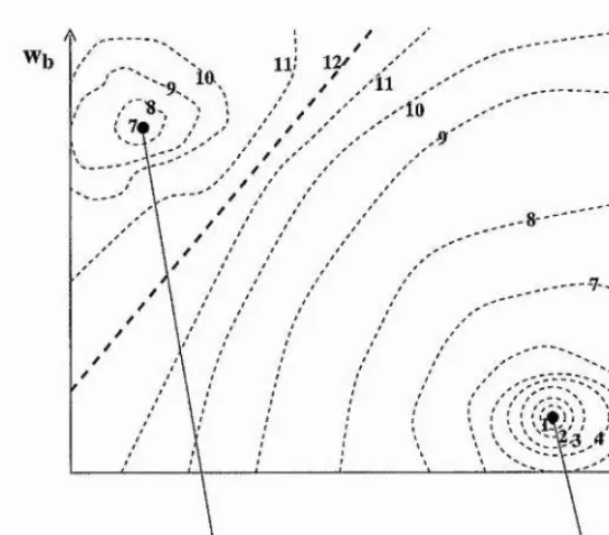
Local Minimum Global Minimum
Figure 2.1; Stylised view of error-weight space with weight axes Wa and Wb and error is indicated by the number on the contour lines. W i is a local minimum and W% is the desired global minimum.
as the theoretically most pure method, takes a step down the surface in the direction in
which the error decreases most steeply.
Error weight surfaces for each pattern individually have empirically been found to be rel
atively simple for gradient descent techniques to traverse. That is local minima, which are
defined as being states on the surface suiTounded by higher error in all directions locally,
while not being the lowest eiTor on the whole surface, have not been reported for these
surfaces. When performing steepest gradient descent on such simple surfaces the global
minimum is usually found in a few iterations of BP. This is also reported by Weir and Chen
in [WC90].
[image:37.613.152.430.67.311.2]Ch a p t e r 2. Co m m o n Ne u r a l Tr a in in g Te c h n iq u e s 25
complex surfaces which are difficult to travel on using gradient descent techniques. One
such complexity is the occunence of local minima in the error-weight surface. Local min
ima have often been reported such as by Brady in [BR8 8] and examined by Sontag and
Sussmann in [SS89]. Figure 2.1 shows what a global and a local minimum may look like
for a neural error weight surface. The problem of performing gradient descent on such an
error weight surface is that once the state is within the local minimum’s basin of attrac
tion, training will eventually get stuck at the local minimum. When initialising the training
process at random states the probability of reaching the desired global minimum is propor
tional to the ratio of the global minimum basin size to the local minimum basin size. For
single layer networks consisting of one neuron only it has been shown that the occuiTence
of multiple local minima is common place. Auer et al reported in [AHW97] that the num
ber of local minima rises exponentially with respect to the dimensionality and number of â input patterns for single neurons. Various examples of local minima for single layer net
works aie also described by Lewis and Weir in [LW99] which present great difficulties for
BP.
The supeiposition of the individual pattern error weight surfaces also creates other dif
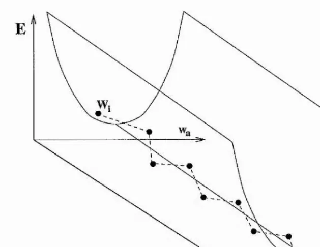
ficulties for gradient descent techniques such as ravines as reported by Weir in [Wei91].
Figure 2.2 is a stylised view of a ravine shaped error weight surface. Following the steepest
descent direction on such ravines will cause a zig-zagging travel path if the step-size is not
exactly such to direct the transition to the centre of the ravine. Each blob on the zig-zag path in Figure 2.2 denotes a state achieved through one single step from the previous state.
E
Figure 2.2: Stylised view of error-weight space with weight axes Wa and Wy and an axis for the error E. Wj denotes an initial starting state and the dashed lines indicate the zig-zag line of travel obtained when following the steepest gradient descent.
must be set low which slows the training process down. The problem is then that training
may often be so slow that a minimum is not found in the time allowed.
Another problem for BP is the occunence of shallow regions on the enor-weight surface
with almost constant high error. Such regions are commonly termed plateaus. When the
error-weight state is situated on such a plateau, training will proceed so slowly, due to the
shallow gradients, that it may take a very long time to reach regions of lower error, and
again a minimum may not be reached in the time allowed.
In [RM8 6] two methods are presented for performing gradient descent using the partial
gradients obtained via BP. One of the methods is off-line BP, also commonly referred to as
Ch a p t e r 2. Co m m o n Ne u r a l Tr a in in g Te c h n iq u e s 27
in which the weights are updated after all the patterns have been presented and the gradients
have been calculated for each weight over all the patterns p according to (2.4). Specifically each weight Wij is then updated in proportion to the calculated gradients, i.e.
dE ^ de^
where wj, is the weight value after the weight transition is made, and rj is the step size of
the weight update, commonly known as the learning rate. This kind of weight update is
equivalent to performing steepest gradient descent and so off-line BP finds surfaces with
plateaus, local minima and ravines difficult to traverse. It is possible to add a momentum
term to the weight update which has been shown to smooth out the oscillations encountered
when travelling on ravines to a limited extent. The smoothing occurs by adding a fraction of
the previous transition direction to the current gradient in the hope that they will cancel out
to provide a transition which does not shoot up the other side of the ravine. A low learning
rate will also reduce the oscillations when travelling on ravines, but will increase the overall
training time and so has to be set with care. In practice a useful learning rate and momentum
setting depends on the shape of the surface. The wrong learning rate and momentum setting
may cause leai'ning to follow oscillatory trajectories of increasing amplitude and bounce
out of the ravine. Ironically this undesired effect has been quoted as being beneficial for
dealing with local minima. High momentum and learning rate may bounce gradient descent
training out of a local minimum’s basin of attraction, but the cause of this success is by
creating training which does not always converge to a minimum in the current basin of
attraction. Hence high momentum and learning rates may likewise bounce the trained state
For on-line BP the procedure is very similar', the only difference being that the weight
update occurs after each pattern is presented. All the weights are updated as follows
/ frs
Compared to batched BP, on-line BP offers the advantage of multiple directions for the
price of one. That is because a different transition direction is explored for every pattern
as it is presented, but the overall cost of computing the gradients is the same as for batched
BP. The drawback of on-line BP is that a good direction for one pattern is not necessarily
a good direction for another pattern and hence multiple oscillations may occur within the
cycle of presenting all the patterns once. The overall merit of one version of BP against
the other appears unclear conceptually. While on-line BP may possibly be more suited for
certain types of training sets batched BP may be better suited for others.
In summary, BP offers a general method for optimisation through enor reduction, but suf
fers from finding complex surface traversal difficult. Its versions of gradient descent fail to
Ch a p t e r 2. Co m m o n Ne u r a l Tr a in in g Te c h n iq u e s 29
2.2 Conjugate Gradient Descent
Conjugate Gradient Descent (COD) is a method to improve on the directions obtained
for training a neural network compared to those obtained using steepest gradient descent.
When performing some version of steepest gradient descent on an error surface, such as
using BP as described in section 2.1, the direction does not generally point towards a min
imum error state on the error-weight surface. Depending on the learning rate and momen
tum setting this often leads to arbitrary oscillations in surface regions with ravines. The
oscillations substantially increase the training time required to reach the global minimum,
provided a local minimum is not reached instead, in which case failure occurs. The basic
idea of COD is to, at each stage, preserve the goodness of previous transitions as much as
possible by choosing successive travel directions which avoid oscillations.
Part of the COD technique uses line minimisation, also referred to as line search, which in
a neural sense is a search for minimum error along a fixed line in weight space. Line search
alone does not improve matters compared to BP, although it achieves maximum goodness
along its direction. If no momentum term is used and the direction for the individual line
search is along the steepest descent direction then each search direction will be orthogonal
to the previous direction as shown in [Pre94]. Even for a simple quadratic 3-D enor-weight
surface, with 2 weight axes and one error axis, the orthogonal directions do not generally
point directly towards the overall global minimum on the surface. Performing iterative line
search on such a surface will then lead to many steps being taken in orthogonal directions
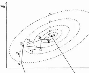
Wb
[image:43.615.144.450.72.323.2]Global Minimum Weight State Initial Weight state
Figure 2.3: Stylised view of weight space with 2 weight axes Wa and Wb- Numbers on the
dashed error contour lines are not to scale but denote the increasing height of this simple quadratic error function around its one minimum which is therefore a global minimum.
Figure 2.3 is a schematic view of 2-D weight space with a quadratic error function of the
weights as the 3"" dimension of the error-weight surface. The direction of increasing error
is denoted by numbers on the dashed error contour lines. When starting at the initial weight
state A and performing line minimisation along the steepest descent direction Vj, B is ob
tained as the minimum eiTor state. It should be noted that the steepest descent direction,
at any state, is orthogonal to the tangent on the error contour line containing the cunent
state. It should also be noted that the minimisation direction forms the tangent to the error
contour line containing the minimum along the minimisation direction. If the minimisa
tion direction is always chosen to be the steepest descent direction, then successive search
directions are necessaiily orthogonal to each other. Thus line searches from B along the
Ch a pt er 2. Com m on Ne u r a l Tr a in in g Te c h n iq u es 31
steepest descent direction at each stage will take the search to the states C, D, E and will
continue in a zig-zag path along the directions Vi and V2, with an ever decreasing step size,
towards the minimum state at G. Following such a path means that a lot more steps are
taken than necessary for such a simple surface.
The other part of the CGD technique offers a way to preserve the goodness achieved
through previous line searches so as to avoid travelling on the zig-zag path just described.
Related to the simple example in Figure 2.3, CGD offers a way to establish a search di
rection V3 for the 2“** line search, when situated at B, which passes through the minimum
at G. When starting at A in Figure 2.3 the initial direction for the line search is chosen to
be along the steepest descent direction vi and so B is the obtained minimum for that line
search. For the second line search CGD allows the calculation of a conjugate direction to
Vi. The conjugate direction to v% is a direction along which the value of the gradient on
the error-weight surface along the Vi direction is the same as it was at B The conjugate
direction at B for Vi and an enor-weight gradient of zero along the Vi direction is Vg, which
passes through the minimum at G and any other line minimisation along the Vi direction,
such as D for example. The 2’“* line search can then be performed along the V3 direction to
obtain the desired minimum weight state at G
In order to calculate the conjugate directions, CGD makes use of 2"‘^ order derivatives of
the eiTor function with respect to the weights. These 2"‘* order derivatives are grouped into
N weight parameters Wi where i can range from 1 .. .N , the Hessian can be written as:
H
-d^E d'^E d^E
dwi^ dwidw2 dWidWj\!
d^E d^E d^E
dW20Wl dw2‘^ dW2dv}N
d^E d'^E d^E
\
(2.7)
y
d w j ^ d w i d w N d v j 2 ’ ’ ’ JFinding the conjugate direction to Vi involves evaluating the Hessian and solving the fol
lowing equation expressed here in matrix notation
Vi HV3 = 0 (2.8)
in terms of the components of the vector V3
V3
f \ Va
\ v , ,
(2.9)
where Va and are values along the Wa and Wb axes in Figure 2.3.
The 2"‘‘ order derivatives of the error function with respect to the weight paiameters in
the Hessian indicate how the gradient on the error-weight surface will vary for changes in
weight. For error-weight surfaces which are quadratic functions of the weight parameters
all entries in the Hessian are constant over all weight settings. The Hessian is an exact
model of the surface shape in this case and CGD is able to find the minimum in at most N
applications of line search for a quadratic error function of N weight parameters.
In order to find a set of conjugate directions it is not necessary to compute the Hessian
explicitly. Instead conjugate directions may be generated as follows. At time f = 1 set the
Ch a p t e r 2. Co m m o n Ne u r a l Tr a in in g Te c h n iq u e s 33
vector of the error derivatives with respect to each weight evaluated at time t = 1, For
subsequent time steps with t > 1, search directions may then be set using
vM = (-VE)I, +
- 1)
(2.10)
where (3{t) is a scalar value much like an adaptive momentum term which adds a fraction
of the previous direction to the cunent steepest descent direction. Many rules have been
developed for computing a suitable such that the directions obtained between time
(t — N + 1) and t are all mutually conjugate. One of these mles is the commonly used
Polak-Ribiere formula from [Pol71].
Using the search directions obtained with (2.10) and (2.11) will lead, just as when calculat
ing the Hessian explicitly, to finding the minimum in as many steps as there are dimensions
in the weight space for quadratic error functions. For non-quadratic error-weight surfaces,
the minimum may not have been reached after this number of steps. In this case the pro
cedure is re-initialised to search along the steepest descent direction from the cunent state
by setting /9(f) to 0 for one step. In successive steps, search is performed along conjugate
directions again by adjusting /^(t) according to (2 .1 1).
CGD is certainly a big improvement for quadratic surfaces compared to using steepest
gradient descent in as much as it is guaranteed to reach the minimum in a low number
of steps. Even for non-quadratic surfaces CGD, would appear to have the advantage of
making use of more information in its search than BP for example.
bined with line search along these directions. Ironically, line search can be a cause of
problems for CGD. Searching for the lowest error along a specific direction can, depend
ing on the surface, lead to travelling large distances in weight space from which training
has to return and may only do so with great difficulty. This can slow down training and
in some cases may prevent CGD from converging to the desired minimum in the allowed
time. From work done in the group here at St. Andrews CGD has been found to be less
robust than BP in these circumstances [WeiOO].
Other difficulties may arise for CGD which originate from the assumption made that the
travel surface is roughly quadratic in shape. If the eiTor surface is more complex and far
from quadratic in shape, the conjugate directions will not point towards the global minimum
after N steps and may not lead to a convergence within the time allowed. Baum and
Lang for example reported in [BL90] that CGD never managed to converge to the global
minimum which is known to exist for the 2-spirals problem for a fixed 2-50-1 network
architecture (2 input units, 50 hidden units and 1 output unit). Such failure is not perhaps
surprising since although CGD is a big improvement for travelling on quadratic surfaces, it
does not overcome the basic limitation of gradient descent techniques and so will still find
Ch a p t e r 2. Co m m o n Ne u r a l Tr a in in g Te c h n iq u e s 35
2.3 Levenberg-Marquardt
Levenberg-Marquardt is a training method which aims to provide an error-weight surface
search, more informed than the techniques described so far, by combining the strengths of
both first order methods, such as gradient descent, and methods which make use of second
order derivative information, when it appears to be useful. As such, Levenberg-Marquardt
is a hybrid method between making use of 2’"^ derivative information in terms of the inverse
of the Hessian and simple steepest gradient descent. For a detailed presentation of the
Levenberg-Marquardt technique see [Pre94].
As shown in section 2.2, the actual implementation of CGD only makes indirect use of
second order derivatives. This is because the Hessian, as shown in (2.7) on page 32, does
not need to be evaluated explicitly to obtain conjugate directions. A method called New
ton’s method on the other hand, which for this discussion can in theory be treated as part of
the hybrid Levenberg-Marquardt technique, does make explicit use of the Hessian matrix.
The idea is that the direction and required step size leading to the global minimum can be
calculated exactly for a quadratic error surface. For a change in the weight state of Aw, the
change in the error gradient AG is
AG = H A w (2.1 2)
where AG is a vector of gradient changes for all weights, H is the Hessian and Aw is a
vector of weight changes for all weights. At a minimum all the enor-weight gradients are
to be equal to the negative of the current error-weight gradient, that is
AG = H A w = - V E (2.13)
where V E is a vector containing the first derivatives of the error function with respect to
all the weights. Re-arranging (2.13) in terms of the change in weight state Aw gives us the
desired weight transition, also known as a Newton step, which has the appropriate step size
and direction to the global minimum for a quadratic surface
Aw = V E (2.14)
where is the matrix inverse of the Hessian.
The basic intuition behind Levenberg-Marquardt is to use information from the inverse
Hessian to perform a Newton step when it is useful to do so, and otherwise to perform
steepest gradient descent. In practice implementations of Levenberg-Marquardt mostly
use an approximation of the inverse Hessian to speed up computation, but the effect on
convergence is the same such that the methods for approximating the inverse will not be
discussed here. If the error E is repeatedly very low, the assumption is made that the currently trained state must be close to the global minimum, in which case the enor-weight
surface is expected to be roughly quadratic in shape. In this case Levenberg-Marquardt
performs a weight adjustment which by approximating the inverse Hessian is very similar
to the above Newton step, which should lead to the global minimum of a quadratic surface.
If on the other hand the enor is repeatedly high, then no assumptions are made about the
Ch a pt er 2. Com m on Neu r a l Tr a in in g Tec h n iq u es 37
direction given by
Aw = -f/V E (2.15)
where rj is the step size, otherwise known as the learning rate.
Being a hybrid method, Levenberg-Marquardt will suffer from problems which affect each
part of the hybrid individually. One possible problem for the Levenberg-Marquardt method
is that on various surfaces the error may be low, while the error surface between the cunent
state and the goal weight state is not at all quadratic in shape. This will certainly occur
when situated near a local minimum with a low error. Here a Newton step does not point
towards the global minimum and will cause convergence to the local minimum.
Alternatively, the shape of the surface may be such that it takes a long time for the enor
to decrease, such as when situated on a high plateau of almost constant error on the error-
weight surface. In this case the transitions performed by Levenberg-Marquardt are mainly
dominated by steepest gradient descent. It is known that shallow gradients, as found on
plateaus, present problems for simple gradient descent techniques, as described in sec
tion 2.1. If the gradient is shallow then it can take many iterations to decrease the eiTor
towards the minimum, in some cases more iterations than allowed. Levenberg-Marquardt
will find surfaces with plateaus difficult to traverse in the initial stages, just as simple gra
dient descent does.
In summary Levenberg-Marquardt offers a way to smoothly vary between an inverse Hes
sian approach perfoiining quadratic descent and steepest gradient descent, but can still
Levenberg-Marquardt is a more sophisticated approach than BP to minimising the enor
function, it does not overcome one of the most basic limitations of gradient descent, namely
that of getting trapped in local minima. The sting of Bianchini’s point in [BFGM98], made
with regard to BP, is still not removed when looking at such more sophisticated training
methods which attempt quadratic descent by approximating the inverse of the Hessian or
alternatively some sort of gradient descent on a fixed error-weight surface. Both parts of
Levenberg-Marquai'dt, that is quadratic descent and steepest gradient descent, are only able
to offer local convergence. Like BP and CGD, Levenberg-Marquardt will still converge to
the attractor of the basin its initial state is contained within and is therefore not able to
overcome the local minimum problem.
2.4 Simulated Annealing
A technique possibly not used for training feedforward neural networks as commonly as
it is used in other areas of optimisation and for training a particular type of neural net
work called a Boltzmann Machine is simulated annealing which originates from work in
[KGV83]. Although it may seem strange to make mention of simulated annealing without
explaining the Boltzmann Machine I wish to place simulated annealing in the framework
of continuous function optimisation which is in theory applicable to training feedforward
neural networks.
The idea for simulated annealing takes its inspiration from engineering and chemical physics,