The impact of the initial condition on covariate augmented unit root tests

The Impact of the Initial Condition on Covariate

Augmented Unit Root Tests

Chrystalleni Aristidou, David I. Harvey and Stephen J. Leybourne

School of Economics, University of Nottingham

January 2016

Abstract

We examine the behaviour of OLS-demeaned/detrended and GLS-demeaned/de-trended unit root tests that employ stationary covariates, as proposed by Hansen (1995) and Elliott and Jansson (2003), respectively, in situations where the mag-nitude of the initial condition of the time series under consideration may be non-negligible. We show that the asymptotic power of such tests is very sensitive to the initial condition; OLS- and GLS-based tests achieve relatively high power for large and small magnitudes of the initial condition, respectively. Combining information from both types of test via a simple union of rejections strategy is shown to e¤ectively capture the higher power available across all initial condition magnitudes.

Keywords: Unit root tests; stationary covariates; initial condition uncertainty; asymp-totic power.

JEL Classi…cation: C22.

1

Introduction

Conventional testing for a unit root in a time series is typically carried out using the OLS-demeaning/detrending procedure of Dickey and Fuller (1979), or the GLS-demeaning/detrending procedure of Elliott, Rothenberg and Stock (1996). When the series under consideration covaries with an available stationary variable, Hansen (1995)

showed that it is possible to substantially increase the power of the OLS-based unit root tests by augmenting the underlying OLS regression model with that stationary covariate. Elliott and Jansson (2003) and Westerlund (2013) show that incorporating covariates in a demeaning/detrending setting also improves the power of GLS-based unit root tests.

As shown in Müller and Elliott (2003), the powers of conventional OLS-based and GLS-based unit root tests are sensitive to the magnitude of the unobserved initial condition of a time series. For a small initial condition, GLS-based tests can have sub-stantially more power than their OLS-based counterparts, while the reverse is true for a large initial condition. Typically, the power of OLS-based tests is an increasing func-tion of this magnitude, whereas GLS-based tests demonstrate the opposite behaviour. In any practical testing situation, the magnitude of the initial condition is not known (nor can it be consistently estimated) and it is therefore unclear whether it is best to apply an OLS- or GLS-based unit root test in order to extract the most information about the presence, or otherwise, of a unit root. Harvey et al. (2009) examine the behaviour of a simple union of rejections strategy whereby (in its simplest guise) the unit root null hypothesis is rejected whenever either of the individual OLS- or GLS-based unit root tests rejects. This procedure is shown to perform well in practice since it captures the superior power of the GLS-based test for a small initial condition and the superior power of the OLS-based test for a large initial condition.

In this paper we show that the patterns of sensitivity of the power of OLS- and GLS-based covariate augmented unit root tests to the magnitude of the initial condition are actually very similar to that of their non-covariate augmented counterparts. This implies that the same considerations are relevant as in the non-covariate augmented case, when deciding which of the OLS- or GLS-based covariate augmented unit root tests to apply. Our proposed solution is once again to employ a union of rejections strategy, which we demonstrate is very e¤ective in the covariate augmented context.

what follows,_I(:)denotes the indicator function,Ldenotes the lag operator,_!p denotes convergence in probability, and₎ denotes weak convergence.

2

The model and covariate augmented unit root

tests

For purposes of transparency we will conduct our analysis within the context of a fairly simple model that admits a single covariate and abstracts from serial correlation in the innovations; we subsequently discuss elaborations to the case of more general serial correlation in section 5 below. We consider the following model for the series yt and

the covariatext, t= 1; :::; T:

" yt xt # = "

y + yt x+ xt

# + " uy;t ux;t # (1) where _"

uy;t uy;t 1 ux;t # = " vt et # : (2)

Within this generic data generating process (DGP) speci…cation we identify three al-ternative speci…cations for the deterministic components of yt and xt, with varying

restrictions concerning the trend component ofyt and xt:

Model A : _y = _x = 0

Model B : y 6= 0; x= 0

Model C : _{y 6}= 0; _x6= 0

In Model A, no trends are assumed present in either yt or xt; in Model B, a trend is

permitted in yt alone, while both yt and xt admit a trend in Model C. We make the

following assumption regarding the innovations vt and et:

Assumption 1. The stochastic process "t = [ vt et ]0 is a martingale di¤erence

sequence with variance E("t"0t) = where

=

" 2

v ev ev 2e

#

and suptE(ketk

4

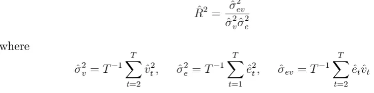
)<₁. Let the squared correlation between the innovation vt and the

covariate ux;t =et be denoted by

R2 =

2

ev

2

v 2e

Within (2), for the autoregressive processuy;t we set = 1 +c=T forc 0, withc= 0

and c <0 corresponding to unit root and local-to-unit root autoregressive processes, respectively. Here ux;t = et is the stationary covariate which is correlated with the

innovation term ofuy;t when ev 6= 0 (i.e. when R2 >0).

In this paper we wish to allow for the possibility that the initial condition of the autoregressive processuy;t, i.e. uy;1, is asymptotically non-negligible, so that its limiting e¤ect on covariate augmented unit root tests can be ascertained. Speci…cally, the following assumption is made regarding the behaviour of uy;1:

Assumption 2. For c < 0, the initial condition is generated according to uy;1 =

p ₂

v=(1 2), where is a …xed parameter. For c= 0, we may set uy;1 = 0 without loss of generality, due to the exact similarity of the covariate augmented unit root tests to the initial condition in this case.

In Assumption 2, the parameter controls the magnitude of the …xed initial condition

uy;1 (i.e. the deviation of the initial observation from the underlying mean/trend in the data) relative to the standard deviation of a stationaryAR(1)process with parameter and innovation variance 2v. This form for the initial condition is closely related to that

given in Müller and Elliott (2003) and Harvey and Leybourne (2005). Notice also that, when c < 0, the initial value is not asympytotically negligible because T 1=2uy;1 !

v=

p

2c asT _{! 1}.

Our focus in this paper is on testing the unit root null H0 : = 1 against the stationary alternativeH1 : <1, in the case where a stationary covariate is available. In the context of the model (1)-(2) and Assumption 1 we now outline statistics that derive from the Hansen (1995) and Elliott and Jansson (2003) approaches to covariate augmented unit root testing, which are respectively based on OLS and GLS detrending of theyt data.

2.1

OLS-based statistics

The Hansen (1995) approach tests for a unit root inytusing a Dickey-Fuller-type

regres-sion, augmented by the stationary covariate as an additional regressor, and implicitly employs OLS demeaning/detrending of the yt and xt series (note that Hansen does

not consider Model C, but extension to this case is trivial). Based on our components representation of the DGP in (1), we express this type of statistic as follows:

t^ =

^

where ^ and s:e:(^)are the OLS estimate and associated standard error of obtained from the regression

^

uy;t= ^uy;t 1+ ^ux;t+ t (3)

withu^y;tandu^x;t denoting residuals from the OLS demeaned/detrendedytandxtseries

^

uy;t =

(

yt ^y for Model A

yt ^y ^yt for Models B, C

^

ux;t =

(

xt ^x for Models A, B

xt ^x ^xt for Model C

where in the demeaned cases, ^_y and ^_x denote the estimated intercepts in the regres-sions ofyt and xt, respectively, on a constant, while in the detrended cases, ^y;^y and

^_x;^_x denote the intercept, trend coe¢ cient estimates in the regressions of yt and xt,

respectively, on a constant and linear trend.

2.2

GLS-based statistics

Elliott and Jansson (2003) propose an approach to covariate augmented unit root test-ing based on a likelihood ratio principle combined with GLS demeantest-ing/detrendtest-ing for

yt but retaining OLS demeaning/detrending for the stationary covariate xt.

Speci…-cally, for our basic model, their statistic is given by

^ =T 8 < :tr 0 @ " _T X t=1 ^

ut(1)^ut(1)0

# 1" _T X

t=1

^

ut( )^ut( )0

#1

A 1

9 = ;

where, forr= = 1 +c=T (for some chosen c <0) and r= 1,

^

ut(r) =zt(r) dt(r)0^(r)

with

zt(r) =

"

(1 r_I(t >1)L)yt

xt

#

dt(r)0 =

8 > > > > > > > > > < > > > > > > > > > : "

1 r_I(t >1) 0

0 1

#

for Model A "

1 r_I(t >1) 0 (1 r_I(t >1)L)t

0 1 0

#

for Model B "

1 r_I(t >1) 0 (1 r_I(t >1)L)t 0

0 1 0 t

#

and

^(r) =

" _T X

t=1

dt(r) ^ 1dt(r)0

# 1" _T X

t=1

dt(r) ^ 1zt(r)

#

where ^ is a consistent estimator of .

An alternative approach to covariate augmented unit root testing that also makes use of GLS demeaning/detrending for yt is to adapt the Hansen (1995)

Dickey-Fuller-based statistic, where the deterministic coe¢ cients in (1) are estimated using GLS rather than OLS, an approach suggested by Westerlund (2013). Speci…cally, we con-sider the following GLS-based variant of Hansen’s statistic:

t~ =

~

s:e:(~)

where ~ and s:e:(~) are obtained from the …tted OLS regression

~

uy;t= ~ ~uy;t 1+ ~^ux;t+ ~t (4)

with u^x;t denoting residuals from the OLS demeaned/detrended xt series as before,

but nowu~y;t denoting the GLS demeaned/detrended yt series, obtained from an OLS

regression of(1 _I(t > 1)L)yt on1 I(t > 1) for Model A, and (1 I(t > 1)L)yt

on[1 _I(t >1);(1 _I(t >1)L)t]0 for Models B and C.

Both the ^ and t~ GLS-based statistics rely on specifying a value of c. Elliott and Jansson (2003) and Westerlund (2013) suggest using the Elliottet al. (1996) values of

c= 7for Model A and c= 13:5 for Models B and C. These choices are motivated by the value ofc=cfor which the nominal 0.05-level asymptotic Gaussian local power envelope is at 0.50 in the non-covariate augmented case, which corresponds to the case of R2 _{= 0 in the context of the covariate augmented tests. As Elliott and Jansson} (2003) and Westerlund (2013) note, it is also possible to selectcaccording to the value of R2_{, so that the asymptotic Gaussian local power envelope is at 0.50 for any given} R2_{, but these authors do not recommend such an approach, arguing that unit root test} power is increasing inR2_{(for a givenc), and so base their choice of a singlecparameter} on the lowest power scenario (R2 _{= 0). In what follows, we follow such previous work} and setc= 7 for Model A and c= 13:5 for Models B and C.

3

Asymptotic results

convergence result

T 1=2

b_XrTc

t=1 " vt et # ) " v 0 eR p ₂

e(1 R2)

# "

W1(r) W2(r)

#

=

"

vW1(r)

e RW1(r) +

p

1 R2_W 2(r)

#

where W1(r) and W2(r) are independent Brownian motions. The initial condition manifests itself via the result (see, for example, Müller and Elliott, 2003)

T 1=2(uy;brTc uy;1)) vKc(r) (5)

where

Kc(r) =

(

W1(r) c= 0

(erc 1)=p 2c+W1c(r) c <0

(6)

and W1c(r) is the Ornstein-Uhlenbeck process

W1c(r) = c

Z r

0

ec(r s)W1(s)ds+W1(r):

The following theorem now provides the limit distributions of the three covariate aug-mented unit root statistics, the proof of which can be found in the companion working paper version Aristidouet al. (2016) [ALT].1

Theorem 1 For the DGP given by (1)-(2), under Assumptions 1 and 2, with = 1 +c=T, c 0,

(i) For Model i (i=A; B; C),

t^ ) c

p

1 R2 qR1

0Lic(r)2dr+

p

1 R2 R1

0 L

i

c(r)dW1(r) qR1

0 Lic(r)2dr

R R1

0 L

i

c(r)dW2(r) qR1

0 Lic(r)2dr

where

LA_c(r) = Kc(r)

R1

0Kc(s)ds LB_c(r) = L_cC(r) =Kc(r)

n

4R₀1Kc(s)ds 6

R1

0sKc(s)ds

o n

12R₀1sKc(s)ds 6

R1

0Kc(s)ds o

r:

1_{Note that the key result (6) which shows how the initial condition enters the limit distributions is}

unchanged if is not a …xed parameter but is instead a random variable. Of course, the limitKc(r)

(ii) For Modeli (i=A; B; C),

t~ )

c

p

1 R2 qR1

0M

i

c;c(r)2dr+

p

1 R2 R1

0 M

i

c;c(r)dW1(r) qR1

0 M

i

c;c(r)2dr

R R1

0 M

i

c;c(r)dW2(r) qR1

0 M

i

c;c(r)2dr

+_p c

2c(1 R2₎ R1

0 M

i c;c(r)dr

qR1 0 M

i

c;c(r)2dr

+_p 1 1 R2

Ni c;c

n

cR₀1rMi c;c(r)dr

R1 0M

i c;c(r)dr

o

qR1 0M

i

c;c(r)2dr

+_p R 1 R2

PiR1

0 M

i

c;c(r)dr+Qi

R1 0 rM

i c;c(r)dr

qR1 0 M

i

c;c(r)2dr

where

M_c;cA(r) = Kc(r)

M_c;cB(r) = M_c;cC(r) =Kc(r)

n

c Kc(1) + 3(1 c )

R1

0sKc(s)ds o

r

N_c;cA = 0

N_c;cB = N_c;cC =c Kc(1) + 3(1 c )

R1

0rKc(r)dr PA = PB =RW1(1) +

p

1 R2_W 2(1) PC = 4nRW1(1) +

p

1 R2_W 2(1)

o

6nRR₀1rdW1(r) + p

(1 R2₎R1

0rdW2(r) o

QA = QB = 0

QC = 12nRR₀1rdW1(r) + p

(1 R2₎R1

0rdW2(r) o

6nRW1(1) +

p

1 R2_W 2(1)

o

with c = (1 c+c2₌₃₎ 1_{(1 c).} (iii) For Model i (i=A; B; C),

^ _)Gi c;c+H

i c;c+

R2

1 R2(c

2 _2cc)R1 0S

i c(r)

2_dr+ R

p

1 R22c R1

0S

i

c(r)dW2(r) where

GA_c;c = c2R₀1Kc(r)2dr cKc(1)

GB_c;c = GC_c;c=c2R₀1Kc(r)2dr+ (1 c)Kc(1)2 kc1

n

(1 c)Kc(1) +c2

R1

0rKc(r)dr o2

H_c;cA = H_c;cC = 0

H_c;cB = k_c1n(1 c)Kc(1) +c2

R1

0rKc(r)dr o2

kc+

c2_R2

12(1 R2₎ 1

(1 c)Kc(1) +c2

R1

0rKc(r)dr+ R2

1 R2

c(c c) 2

R1

0Kc(r)dr c(c c) R1

0rKc(r)dr

+_p R 1 R2

n

cR₀1rdW2(r) c

2

R1

S_cA(r) = S_cB(r) =Kc(r)

R1

0Kc(s)ds S_cC(r) = Kc(r) (4 6r)

R1

0Kc(s)ds (12r 6) R1

0sKc(s)ds with kc= 1 c+c2=3.

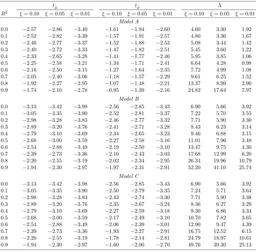
We now consider numerical results for the asymptotic properties of the tests pre-sented so far in this paper. In Table 1 we report asymptotic null (left-tail) critical values for R2 ₌

f0;0:1; :::;0:9_g for all tests at the nominal 0.10-, 0.05- and 0.01-levels, which were obtained by direct simulation of the limit representations of Theorem 1 with c= 0 (note from (6) that the limits are not dependent on whenc= 0). For all asymptotic results in this paper, we conducted Monte Carlo simulations using Gauss 9.0 with 50,000 replications, approximating the Brownian motion processesW1(r)and W2(r)using independentN IID(0;1)random variates for each, and approximating the corresponding integrals by normalized sums of 2000 steps.

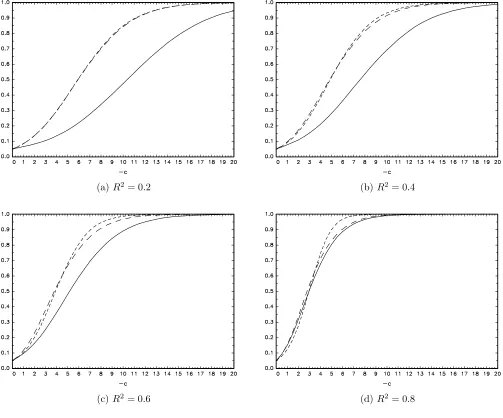
To gain some insight into the relative power performance of the three tests t^, t~ and ^, we …rst abstract from the e¤ect of the initial condition by making the usual assumption that it is asymptotically negligible. The limit distributions of the statistics are then as given in Theorem 1 on setting = 0. Figures 1 and 2 show the local asymptotic powers of the tests conducted at the nominal 0.05-level as functions of

c = _f0;0:5; :::;20:0_g (with c = 0 corresponding to asymptotic size, i.e. 0.05) for Models A and B, respectively, forR2 ₌

f0:2;0:4;0:6;0:8_g.

Consider …rst the results for Model A in Figure 1. We observe that for smaller values ofR2_{, the familiar result of the GLS-based tests delivering a substantial power} advantage relative to the OLS-based test t^ is borne out. These power advantages, however, diminish as R2 _{increases, so that by R}2 _{= 0:8, there is considerably less} di¤erence between the power pro…les of the three tests. For the two GLS-based tests, there is very little to choose between them for small to moderateR2_{, while for larger} R2_{, the ^ test has slightly lower power than t}

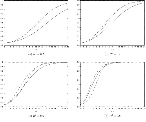
~ for small c but modestly higher power for some larger c. In Figure 2 (Model B), as expected we see a reduction in power of all tests relative to Model A, brought about by the allowance of a trend in

yt. However, it is still the case that for small R2, the GLS-based tests outperform

t^, and have similar levels of power to each other. Interestingly, as R2 increases, t~ becomes generally more powerful than ^, and byR2 _{= 0:8, the relative power levels of}

^ _{have reduced to values generally below those of the OLS-based testt^. In contrast,}

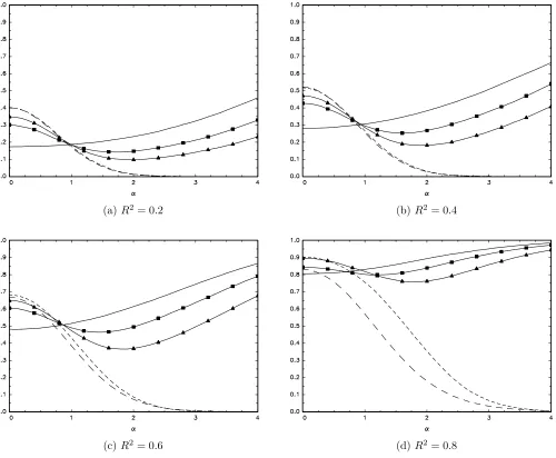
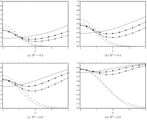
We now examine the e¤ects of an asymptotically non-negligible initial condition on local asymptotic power. Figures 3 and 4 report local asymptotic powers of the …ve tests conducted at the nominal 0.05-level, as functions of = _f0;0:1; :::;4:0_g ( = 0

corresponding to an asymptotically negligible initial condition); note that replacing with would give the same results. Figure 3 presents results for Model A, where a representative local alternative setting of c= 5 is used, while Figure 4 gives results for Model B usingc= 10.

Considering …rst Model A in Figure 3, the stand out feature of these power curves is that while the power of the OLS-basedt^ test is increasing in the magnitude of the initial condition , the powers of both GLS-based tests decrease to zero as increases. Hence, while the GLS tests are more powerful for = 0 (cf. Figure 1) and for small values of , they are much less powerful than t^ for larger initial conditions. This pattern of results closely mirrors what is found when analyzing the e¤ects of initial conditions on standard, non-covariate augmented OLS and GLS demeaned/detrended unit root tests, and highlights the fact that GLS-based unit root tests do not deliver reliable unit root test inference in the presence of large initial conditions. Between the two GLS-based tests, there is little di¤erence between the power pro…les for R2 = 0:2

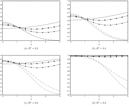
and R2 = 0:4, while as R2 increases to 0:6 and then 0:8, it is clear that ^ emerges as the more powerful procedure. For Model B (Figure 4), we observe the same broad patterns of results vis-à-vis the power of t^ compared to the GLS-based tests. Once again, t^ has power that increases in , while the GLS-based tests have higher power when = 0, but then a decreasing power pro…le as rises. Between the GLS-based tests, in contrast to Model A, here we see that t~ o¤ers generally the best levels of power across , particularly for larger and R2 values.2

4

A union of rejections strategy

The results of the previous section demonstrate that when the initial condition is small, we would want to apply one of the two GLS-based tests (t~ or ^); on the other hand, when the initial condition is larger, applying such a test would result in a (potentially substantial) loss of power relative to applying the OLS-based testt^. In practice, given

2_{In ALT, results are also provided for Model C. Similar comments apply as for Model B in Figure}

2, although forR2_{= 0:8, the power oft}

~ also drops slightly below that oft^, so that heret^ generally

outperforms both GLS-based tests. The power pro…les for Model C across again highlight that the GLS-based tests are typically more powerful thant^ for zero and small , with the reverse ranking for

larger . As with Model A, the powers of the two GLS-based tests are very similar forR2_=f0:2;0:4g,

uncertainty regarding the magnitude of the initial condition, we wish to have available a procedure that capitalizes on both the relatively high power of the GLS approach when is small, and the relatively high power of t^ otherwise. A similar issue arises in the case of non-covariate augmented unit root testing, and the approach proposed by Harveyet al. (2009) is to take aunion of rejections of the OLS- and GLS-based tests, whereby the null hypothesis is rejected if either of the individual tests rejects. In the present context, this implies taking a union of rejections betweent^ and either one of the GLS-based tests.

We now set out the union of rejections approach based on t^ (here denoted by tOLS) and a GLS-based test (t~ or ^) denoted by tGLS. Denoting the asymptotic

-level critical values of these tests by cvOLS and cvGLS, respectively, we can de…ne the simple union of rejections strategy by the decision rule

RejectH0 if ftOLS < cvOLS ortGLS < cvGLSg:

An alternative way of representing this decision rule is to express it in terms a single test statistic,tU R, as follows:

RejectH0 if (

tU R = min tOLS;

cvOLS

cvGLStGLS

!

< cvOLS )

:

If we use_LOLS _and

LGLS _{to denote the generic joint limit distributions oft}

OLS andtGLS,

respectively (i.e. the right-hand-side expressions given in Theorem 1), an application of the continuous mapping theorem establishes that

tU R )min LOLS;

cvOLS cvGLSL

GLS

! :

The Bonferroni bound for the asymptotic size of this procedure under the null is 2

(since it simply involves rejecting the null when either of the individual tests reject). Harvey et al. (2009) suggest restoring the union of rejections asymptotic size to the nominal level by applying a common positive scaling constant, >1, to the (nega-tive) critical valuescvOLS _{and cv}GLS _{(so that t}

OLS is compared with cvOLS and tGLS

with cvGLS_{), such that in the limit, rejection of the null occurs with probability .}

While this approach extends naturally to the covariate augmented unit root testing problem when using t~ for tGLS, since here both cvOLS and cvGLS are negative, we

to bothtGLS and cvGLS, say tGLS and cvGLS , such that the GLS-based test

decision rule is unchanged, but that the adjusted critical valuecvGLS equalscvOLS, i.e. =cvGLS cvOLS. Once the critical values are lined up in this way, the critical values are both negative, and a Harveyet al. (2009)-type multiplicative scaling can be applied to control the asymptotic size. More formally we propose the following union of rejections decision rule:

RejectH0 if ftOLS < cvOLS ortGLS < cvOLSg

or, equivalently,

Reject H0 if tU R = min (tOLS; tGLS )< cvOLS :

In the limit we obtain

t_{U R )}min _LOLS;_LGLS

and we compute by simulation of the limit distribution of t_{U R}, calculating the -level null critical value for this distribution, say cvU R_{, and then evaluate as =}

cvU R_=cvOLS_{. In what follows, we consider two union of rejections procedures, one based}

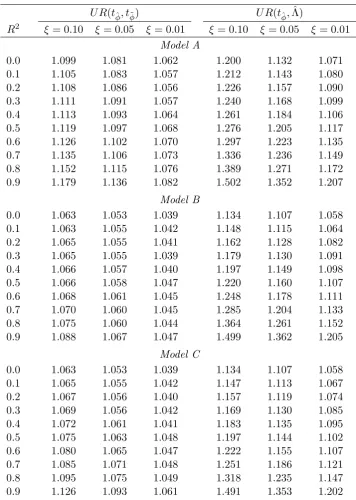
on a union oft^ andt~, the other based on a union oft^ and ^; hereafter we denote these unions byU R(t^; t~)andU R(t^;^ )respectively. Values for forR2 =f0;0:1; :::;0:9g at the nominal 0.10-, 0.05- and 0.01-levels are given in Table 2 for each of these union of rejections strategies.

The union of rejection strategies U R(t^; t~) and U R(t^;^ ) are by construction asymptotically correctly sized. We now consider the asymptotic local power prop-erties ofU R(t^; t~)and U R(t^;^ ) in relation to the powers of the individual tests, the results for which are also displayed in Figures 3-4. Consider …rst Model A in Figure 3, and to aid comparison of the union of rejections procedures, consider an informal (and infeasible) power “envelope”formed from the limit power of ^ for values of up to the point where ^ andt^ have the same power, and from the limit power oft^ for beyond this point. With reference to this envelope, both U R(t^; t~) and U R(t^;^ ) track its broad shape, o¤ering decent power levels across the range of values considered. Both

while in the larger- range where U R(t^; t~) outperforms U R(t^;^ ), the gains can be quite substantial. For this reason, we consider thatU R(t^; t~)o¤ers the more preferable power pro…le of the two procedures across the range of considered. Indeed, it could be argued that overallU R(t^;^ )has an inferior power pro…le to that oft^ alone, due to the relatively low power levels for modest to large . On the other hand,U R(t^; t~)has a power pro…le closer to that oft^ than does U R(t^;^ ) for this region of , while still achieving much of the power gains oft~ overt^ when is closer to zero. This union of rejections therefore o¤ers decent power gains overt^ for the arguably more typical case of small , while simultaneously providing insurance against the low power for large that is associated with t~. For Model B in Figure 4, broadly similar comments can be applied, with U R(t^; t~) outperforming U R(t^;^ ) overall, and U R(t^; t~) having a power pro…le that more closely tracks the shape of the informal envelope comprised of the best performing tests for each region of . If anything, compared to Model A, the power di¤erences between U R(t^; t~) and the informal envelope are less marked, adding weight to our recommendation forU R(t^; t~).3;4

5

Finite sample comparisons

In this section we consider the …nite sample behaviour of the individual tests of section 2 and the proposed union of rejections procedures U R(t^; t~) and U R(t^;^ ) under Assumptions 1 and 2. In order to implement the tests in such a setting, we …rst require a consistent estimator ofR2, given that all the tests have critical values that depend on this unknown quantity (the union of rejections procedures also require R2-dependent scaling values ). Under our assumptions, the estimator

^

R2 = ^

2

ev

^2_v^2_e

where

^2_v =T 1

T

X

t=2

^

v2_t; ^2_e =T 1

T

X

t=1

^

e2_t; ^ev =T 1 T

X

t=2

^

et^vt

3_{Results for Model C are again provided in ALT, and similar comments apply as for Model B in}

Figure 4.

4_{We also considered a variant of theU R(t}

^; t~)procedure where the asymptotic size is controlled

using only a multiplicative scaling tocvOLS _andcvGLS_{as in Harveyet al. (2009). We found that such}

a variant led to near identical local asymptotic power pro…les to those displayed in Figure 4 (Model B). In the case of Figure 3 (Model A),U R(t^; t~)yielded slight local asymptotic power advantages

over this variant for larger values of , while surrendering very little power toU R(t^; t~)for small ,

withe^t= ^ux;t and ^vt being the residual from a regression ofu^y;t onu^y;t 1 can be shown to provide a consistent estimator ofR2. Additionally, as highlighted in section 2.2, the

^ _{statistic requires a consistent estimator of . Given that is also comprised of} 2

v,

2

e and ev, a natural estimator is to use

^ =

"

^2_v ^ev

^ev ^2e

#

which can be shown to be consistent for . Note that bothR^2 and ^ remain consistent when in Assumption 2 is not equal to zero; in contrast, the corresponding estimators outlined in Elliott and Jansson (2003, p.81) are only consistent under the local-to-unit root alternative when the initial condition is asymptotically negligible (i.e. = 0), due to their reliance on a …rst di¤erence-based (cf. GLS-based) demeaning/detrending of

yt.

Our Monte Carlo simulations are based on generating (1)-(2) for T = 150 using 50,000 replications, with "t = [ vt et ]0 IIN(0; ), 2v = 2e = 1, 2ev = R2 =

f0:2;0:4;0:6;0:8_g, and with y = y = x = x = 0. We …rst simulated the empirical

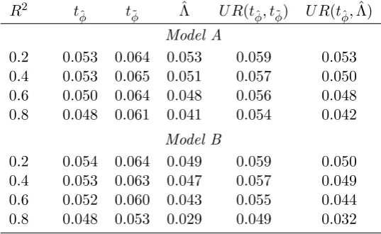
size of the t^, t~, ^ tests and the U R(t^; t~), U R(t^;^ ) procedures at the nominal 0.05-level, setting = 1 in (2). Asymptotic critical values and values were used, linearly interpolating between the values in Tables 1 and 2 on the basis of R^2. The results for Models A and B are reported in Table 3, and we observe only modest …nite sample size distortions across the di¤erent tests and values ofR2. For largerR2 in the case of Model B, ^ and U R(t^;^ ) are a little under-sized, while t~ and U R(t^; t~)are a little over-sized for all cases. However, all sizes for t~ and U R(t^; t~) are below 0.07 and 0.06 respectively, hence …nite sample size distortion does not appear to be a major concern for these procedures.5

Of most interest are the relative …nite sample powers of the procedures, and Figure 5 presents results for Model A, for settings that correspond to the local asymptotic power results in Figure 3. Here, we set = 1 + c=T with c = 5, and report the estimated powers of nominal 0.05-level tests across = _f0;0:1; :::;4:0_g. We …nd that the relative …nite sample powers bear a very close resemblance to the corresponding local asymptotic results, with the powers of t^ increasing in , the powers of t~ and

^ _{initially higher than that for t^ for small , but then falling towards zero as}

increases, and theU R(t^; t~) and U R(t^;^ ) procedures capturing a proportion of the higher t~ and ^ power for small , and a proportion of the higher power of t^ for larger . Compared to the asymptotic results,t~ and U R(t^; t~)appear to have higher

relative power forT = 150, which arises as a result of the small over-size seen for these procedures, but otherwise the …nite sample and large sample results are very similar. What is clear is that the union of rejections procedures o¤er robust power pro…les across the full range of initial conditions, avoiding the low power that can arise from use of the GLS-based tests alone while retaining a good proportion of the additional power o¤ered by the GLS-based tests over the OLS-based variant. Of the two, U R(t^; t~) emerges as the test with arguably the most attractive power properties overall, and on the basis of both the asymptotic and …nite sample results, it is this procedure that we recommend for practical applications.6

In practice, when implementing U R(t^; t~) we would want to allow for additional serial correlation inuy;t and ux;t. In order to admit more general serial correlation into

our DGP, we consider the following simple autoregressive-based extension to (2): "

a(L)(uy;t uy;t 1) b(L)ux;t

# = " vt et # with

a(L) = 1 a1L ::: apLp;

b(L) = 1 b1L ::: bqLq

where the roots ofa(L)andb(L)all lie outside the unit circle, and where"t= [ vt et ]0

continues to satisfy Assumption 1. We also modify Assumption 2 so that, whenc <0,

uy;1 = p

!2₌₍₁ 2_{), where !}2 _{denotes the long run variance of a(L)} 1_v

t, i.e. !2 =

2

v=a(1)2.

In this setting, consider t^ and t~ statistics, computed as in section 2 but on re-placing (3) and (4) with the …tted regressions

^

uy;t = ^ ^uy;t 1+

p

X

j=1

^j u^y;t j+ q

X

j=0

^_{ju^x;t j+ ^}

t; (7)

~

uy;t = ~ ~uy;t 1+

p

X

j=1

~j u~y;t j+ q

X

j=0

~_{ju^x;t j+ ~}

t: (8)

It can then be shown that the large sample results fort^,t~ andU R(t^; t~)from sections 3 and 4 continue to hold.7 _{Moreover, R}2 _{is now consistently estimated using the form}

6_{Results for Models B and C are reported in ALT, and similar comments apply, con…rming our}

preference forU R(t^; t~).

7_{Note that extension of the} ^ _{statistic to the case of additional serial correlation is more involved,}

ofR^2 given in the previous section, but withe^tandv^t replaced with residuals fromq’th

andp+ 1’th order autoregressions …tted tou^x;t andu^y;t, respectively. In practice, since

p and q are unknown, they can be determined endogenously using typical lag order selection rules such as downward testing or application of an information criterion. Finally, note that the …tted regressions (7) and (8) also cover the case where[uy;t; ux;t]0

follows a standard vector autoregression (VAR) process of ordermin(p+ 1; q). In this case, (7) and (8) then model the single equation for uy;t from the VAR, cf. Hansen

(1995), and the contemporaneous regressoru^x;t is not required in (7) and (8).

6

Conclusion

In this paper we have considered the power of covariate augmented unit root tests, based on OLS demeaning/detrending and GLS demeaning/detrending, in the presence of asymptotically non-negligible initial conditions. We have shown that while the GLS-based approaches display superior …nite sample and local asymptotic power for zero and small initial conditions, the power of such procedures falls towards zero as the initial condition increases in magnitude. Since we cannot be sure that such large initial conditions will not arise, this limits the reliability of such GLS-based tests in practice. On the other hand, while the OLS-based variants lose power for small initial conditions relative to their GLS-based counterparts, this ranking is reversed for larger initial conditions as the power of the OLS-based tests increases with the initial condition magnitude. We have then proposed a union of rejections based procedure, which detects evidence in favour of the alternative hypothesis taken from both OLS- and GLS-based demeaned/detrended variants, and …nd that such a procedure works very well, retaining attractive power levels across zero, small and large initial condition magnitudes. Our …ndings mirror those found in the standard non-covariate augmented unit root testing environment, and our recommended procedure adds to the suite of available unit root testing procedures a covariate augmented approach that o¤ers reliable power levels across the range of possible (unknown) initial conditions.

References

Aristidou, C., Harvey, D.I. and Leybourne, S.J. (2016). The impact of the initial condition on covariate augmented unit root tests. Granger Centre Discussion Paper No. 16/01, School of Economics, University of Nottingham.

time series with a unit root. Journal of the American Statistical Association 74, 427–431.

Elliott, G. and Jansson, M. (2003). Testing for unit roots with stationary covariates. Journal of Econometrics 115, 75–89.

Elliott, G., Rothenberg, T.J. and Stock, J.H. (1996). E¢ cient tests for an autoregres-sive unit root. Econometrica 64, 813–836.

Hansen, B.E. (1995). Rethinking the univariate approach to unit root testing. Econo-metric Theory 11, 1148–1171.

Harvey, D.I. and Leybourne, S.J. (2005). On testing for unit roots and the initial observation. Econometrics Journal 8, 97–111.

Harvey, D.I., Leybourne, S.J. and Taylor, A.M.R. (2009). Unit root testing in practice: dealing with uncertainty over the trend and initial condition (with commentaries and rejoinder). Econometric Theory 25, 587–667.

Müller, U.K. and Elliott, G. (2003). Tests for unit roots and the initial condition. Econometrica 71, 1269–1286.

Table 1. Asymptoticξ-level critical values of covariate augmented unit root tests

t_φˆ t_φ˜ Λˆ

R2 ξ = 0.10 ξ= 0.05 ξ= 0.01 ξ = 0.10 ξ = 0.05 ξ= 0.01 ξ= 0.10 ξ = 0.05 ξ = 0.01

Model A

0.0 −2.57 −2.86 −3.40 −1.61 −1.94 −2.60 4.60 3.30 1.92

0.1 −2.52 −2.82 −3.39 −1.57 −1.91 −2.57 4.80 3.36 1.67

0.2 −2.46 −2.77 −3.37 −1.52 −1.88 −2.53 5.08 3.44 1.42

0.3 −2.40 −2.72 −3.33 −1.47 −1.82 −2.51 5.45 3.60 1.22

0.4 −2.33 −2.65 −3.28 −1.41 −1.77 −2.46 5.95 3.85 1.06

0.5 −2.25 −2.58 −3.21 −1.34 −1.71 −2.41 6.64 4.28 0.98

0.6 −2.16 −2.50 −3.15 −1.27 −1.64 −2.35 7.72 4.99 1.08

0.7 −2.05 −2.40 −3.06 −1.18 −1.57 −2.29 9.61 6.25 1.52

0.8 −1.92 −2.27 −2.95 −1.07 −1.48 −2.21 13.37 8.99 2.90

0.9 −1.74 −2.10 −2.78 −0.95 −1.39 −2.16 24.82 17.64 7.97

Model B

0.0 −3.13 −3.42 −3.98 −2.56 −2.85 −3.43 6.90 5.66 3.92

0.1 −3.05 −3.35 −3.90 −2.52 −2.81 −3.37 7.22 5.70 3.55

0.2 −2.98 −3.28 −3.83 −2.46 −2.77 −3.32 7.71 5.90 3.30

0.3 −2.89 −3.20 −3.76 −2.41 −2.71 −3.28 8.43 6.23 3.14

0.4 −2.79 −3.10 −3.69 −2.34 −2.65 −3.23 9.46 6.88 3.15

0.5 −2.68 −3.00 −3.59 −2.27 −2.58 −3.16 11.01 7.96 3.48

0.6 −2.54 −2.88 −3.49 −2.19 −2.50 −3.10 13.47 9.75 4.30

0.7 −2.39 −2.73 −3.36 −2.10 −2.43 −3.03 17.68 12.99 6.20

0.8 −2.20 −2.55 −3.19 −2.02 −2.34 −2.95 26.34 19.96 10.79

0.9 −1.94 −2.30 −2.97 −1.97 −2.31 −2.91 52.20 41.10 25.74

Model C

0.0 −3.13 −3.42 −3.98 −2.56 −2.85 −3.43 6.90 5.66 3.92

0.1 −3.05 −3.35 −3.90 −2.50 −2.79 −3.35 7.24 5.71 3.64

0.2 −2.98 −3.28 −3.83 −2.43 −2.74 −3.30 7.71 5.90 3.38

0.3 −2.89 −3.20 −3.76 −2.35 −2.67 −3.24 8.36 6.27 3.29

0.4 −2.79 −3.10 −3.69 −2.27 −2.59 −3.18 9.30 6.86 3.34

0.5 −2.68 −3.00 −3.59 −2.17 −2.49 −3.10 10.70 7.82 3.65

0.6 −2.54 −2.88 −3.49 −2.06 −2.39 −3.01 12.90 9.47 4.39

0.7 −2.39 −2.73 −3.36 −1.93 −2.27 −2.91 16.75 12.52 6.15

0.8 −2.20 −2.55 −3.19 −1.78 −2.14 −2.81 24.79 18.97 10.61

Table 2. Asymptoticψ_ξ values for ξ-level union of rejections procedures

U R(t_φˆ, t˜_φ) U R(tˆ_φ,Λ)ˆ

R2 _{ξ = 0.10 ξ= 0.05 ξ= 0.01 ξ = 0.10 ξ = 0.05 ξ= 0.01} Model A

0.0 1.099 1.081 1.062 1.200 1.132 1.071

0.1 1.105 1.083 1.057 1.212 1.143 1.080

0.2 1.108 1.086 1.056 1.226 1.157 1.090

0.3 1.111 1.091 1.057 1.240 1.168 1.099

0.4 1.113 1.093 1.064 1.261 1.184 1.106

0.5 1.119 1.097 1.068 1.276 1.205 1.117

0.6 1.126 1.102 1.070 1.297 1.223 1.135

0.7 1.135 1.106 1.073 1.336 1.236 1.149

0.8 1.152 1.115 1.076 1.389 1.271 1.172

0.9 1.179 1.136 1.082 1.502 1.352 1.207

Model B

0.0 1.063 1.053 1.039 1.134 1.107 1.058

0.1 1.063 1.055 1.042 1.148 1.115 1.064

0.2 1.065 1.055 1.041 1.162 1.128 1.082

0.3 1.065 1.055 1.039 1.179 1.130 1.091

0.4 1.066 1.057 1.040 1.197 1.149 1.098

0.5 1.066 1.058 1.047 1.220 1.160 1.107

0.6 1.068 1.061 1.045 1.248 1.178 1.111

0.7 1.070 1.060 1.045 1.285 1.204 1.133

0.8 1.075 1.060 1.044 1.364 1.261 1.152

0.9 1.088 1.067 1.047 1.499 1.362 1.205

Model C

0.0 1.063 1.053 1.039 1.134 1.107 1.058

0.1 1.065 1.055 1.042 1.147 1.113 1.067

0.2 1.067 1.056 1.040 1.157 1.119 1.074

0.3 1.069 1.056 1.042 1.169 1.130 1.085

0.4 1.072 1.061 1.041 1.183 1.135 1.095

0.5 1.075 1.063 1.048 1.197 1.144 1.102

0.6 1.080 1.065 1.047 1.222 1.155 1.107

0.7 1.085 1.071 1.048 1.251 1.186 1.121

0.8 1.095 1.075 1.049 1.318 1.235 1.147

Table 3. Finite sample size of nominal 0.05-level covariate augmented unit root tests: T = 150

R2 tˆ_φ t_φ˜ Λˆ U R(tˆ_φ, t_φ˜) U R(tˆ_φ,Λ)ˆ

Model A

0.2 0.053 0.064 0.053 0.059 0.053

0.4 0.053 0.065 0.051 0.057 0.050

0.6 0.050 0.064 0.048 0.056 0.048

0.8 0.048 0.061 0.041 0.054 0.042

Model B

0.2 0.054 0.064 0.049 0.059 0.050

0.4 0.053 0.063 0.047 0.057 0.049

0.6 0.052 0.060 0.043 0.055 0.044

(a)R2_{= 0}._{2 (b)}R2_{= 0}.₄

(c)R2_{= 0}._{6 (d)}R2_{= 0}.₈

Figure 1. Local asymptotic power of nominal 0.05-level tests: Model A, α= 0;

-(a)R2_{= 0}._{2 (b)}R2_{= 0}.₄

(c)R2_{= 0}._{6 (d)}R2_{= 0}.₈

Figure 2. Local asymptotic power of nominal 0.05-level tests: Model B, α = 0;

-(a)R2_{= 0}._{2 (b)}R2_{= 0}.₄

(c)R2_{= 0}._{6 (d)}R2_{= 0}.₈

Figure 3. Local asymptotic power of nominal 0.05-level tests: Model A, c=−5;

(a)R2_{= 0}._{2 (b)}R2_{= 0}.₄

(c)R2_{= 0}._{6 (d)}R2_{= 0}.₈

Figure 4. Local asymptotic power of nominal 0.05-level tests: Model B, c=−10;

(a)R2_{= 0}._{2 (b)}R2_{= 0}.₄

(c)R2_{= 0}._{6 (d)}R2_{= 0}.₈

Figure 5. Finite sample power of nominal 0.05-level tests: Model A, T = 150,c=−5;