Train composition using motion as a common context

University of Twente

Computer Science

Train Composition

Using Motion as a Common Context

Master Thesis

June 18, 2010

Author P.J. Bakker

Supervisors Ir. J. Scholten

Abstract

The research we conducted and describe in this thesis involves the autonomous discovery of the composition of a train. Using wireless sensor nodes equipped with 3D accelerometers, we aim to use motion as the common context for the correlation of the wagons behind a train.

The draft of the European Rail Track Management System (ERTMS) level 3 specifies a train should be able to be aware of the composition of the train. Since freight trains do not have any form of electrical connection between the freight wagons, either electrical connections should be made or a wireless solution should be developed to be able to detect the train composition. The goal of our research is the development of a wireless system capable of sensing and reporting the train composition.

The lack of electrical connections introduces one of our challenges: energy consumption. Since freight trains are scheduled for maintenance every six to twelve months and there is a lack of a continuous power supply, the train composition system should be energy efficient. An energy efficient system implies using a minimal amount of computational power. Our research is based on building a system using energy efficient wireless sensor nodes.

In the first part of our research, we establish the means we are able to use for identifying two wagons behind the same train. Based on previous research, we use correlation of the filtered data from an accelerometer. We show it is possible to use the Pearson product-moment correlation coefficient, but besides that, we show the use of an optimized version of this correlation coefficient.

For our algorithm, we implemented two methods. Our first solution uses the Pearson correlation coefficient over a growing correlation window. This approach enables very fast response times at the expense of computational power. Our second solution implements the optimized version of the correlation coefficient. Using the optimized version, less computational power is required per node, but the response time has a lower bound of 5 seconds.

Simulation results show that both approaches are applicable; the wireless sensor nodes are able to perform the necessary calculations and determine the train composition within a given time window of 15 seconds. Our fast approach is able to deliver the train composition after just two seconds, given trains with not near identical acceleration characteristics.

4

Contents

1 INTRODUCTION ... 6

1.1 CONTEXT AWARE PERVASIVE SYSTEMS ... 6

1.2 TRAIN SAFETY SYSTEMS... 6

1.3 RELATED WORK ... 7

1.4 PROBLEM STATEMENT ... 7

1.5 CHALLENGES ... 8

1.5.1 Correlation using accelerometers ... 8

1.5.2 Train composition discovery algorithm ... 9

1.5.3 Usability on wireless sensor nodes ... 9

1.6 APPROACH ... 10

1.7 OUTLINE ... 11

2 DATA COLLECTION ... 12

2.1 REQUIREMENTS DATASETS ... 12

2.2 TRAIN AND TRACK ... 12

2.3 HARDWARE... 13

2.4 SOFTWARE... 14

2.5 MEASURING ... 15

2.5.1 Dataset 1 ... 15

2.5.2 Dataset 2 ... 16

2.5.3 Dataset 3 ... 16

2.6 VERIFICATION DATASETS ... 16

3 DATA ANALYSIS ... 18

3.1 RAW DATA ... 18

3.1.1 Output accelerometers ... 18

3.1.2 Frequency spectrum ... 20

3.2 CORRELATION FILTERED DATA ... 21

3.3 CONCLUSIONS ... 28

4 TRAIN COMPOSITION ALGORITHM ... 29

4.1 PAIRING ... 29

4.1.1 Wake-up ... 29

4.1.2 Master/slave ... 29

4.2 CORRELATION ... 30

4.2.1 Correlation algorithm ... 30

4.2.2 Window size ... 32

4.3 TRAIN COMPOSITION ... 32

5 SIMULATION ... 34

5.1 NETWORK ... 34

5.1.1 LogNormal Shadowing ... 34

5.1.2 Acknowledgment and retransmission ... 35

5.1.3 Packet size... 35

5.2.1 Train and node layout... 36

5.2.2 Train movement ... 37

5.2.3 Shunting yard ... 37

5.3 RESULTS ... 38

5.3.1 Correlation ... 38

5.3.2 Master/slave roles ... 40

5.3.3 Network ... 42

6 REALISATION ... 44

6.1 FIXED-POINT CALCULATIONS ... 44

6.1.1 Correlation ... 44

6.1.2 Filter ... 45

6.2 RESOURCES ... 46

6.2.1 Clock-cycles ... 46

6.2.2 Memory ... 47

6.2.3 Network ... 48

7 CONCLUSIONS ... 49

7.1 HYPOTHESIS ... 49

7.2 ALGORITHM ... 50

7.3 USABILITY ... 50

7.4 OVERALL CONCLUSION ... 51

7.5 RECOMMENDATIONS AND FUTURE WORK ... 51

6

Chapter One

Introduction

Relating two objects can be easy for an outsider who is able to observe these two objects and identify a common feature between these two objects. On the other hand, when these two objects need to relate autonomously this can be a challenge. In this chapter, we will show the challenges that rise when two random train wagons need to decide whether they relate or not and we will explain why two trains wagons want to relate in the first place.

1.1

Context Aware Pervasive Systems

Embedding small processing devices in objects and activities as means of improving the use or quality of these objects and activities is a generally accepted way of improving everyday life. The processing devices embed in objects and activities are referred to as pervasive systems [1] or ubiquitous computing [2]. For these devices to be able to assist in everyday tasks one of the challenges is finding out where a device is located. Besides that, the discovery of nearby devices as well as nearby resources are also important aspects. The discovery of location, neighbors and resources is also referred to as context awareness [3].

In this work we research the possibility of a context aware pervasive system as a means of discovering whether two objects are moving together. The example used throughout this research is the discovery of the composition of a train i.e. whether or not it is possible for wagons behind a train to acknowledge they are behind the same train and distinguish them from wagons behind other trains. In the following section, we explain why it is relevant a train is able to autonomously detect the composition of the train.

1.2

Train Safety Systems

The rail system in Europe currently consists of multiple different safety systems: the countries still rely mostly on a country-specific system. International European trains have multiple systems onboard to be able to pass borders and enter another country and hence another safety system. Currently, several running projects in different European countries are in place to deploy a uniform system [4], European Rail Train Management System (ERTMS), under

supervision of the European Railway Agency [5]. The eventual goal is the adoption of the system in all participating countries. The draft for the latest version of ERTMS is known as ERTMS level 3. ERTMS level 1 and level 2 still consider track sections instead of trains as sections, thus implying that a small light train takes an even amount of space as a large and heavy train. ERTMS level 3 introduces the possibility to consider a train as a moving block, keeping a certain amount of space in front as well as the back of the train thus forming a safety zone around the train.

the side of track for the indication of the availability of the next zone, whereas ERTMS level 2 communicates this information by radio using GSM-Rail (GSM-R). Freight train wagons use a simple steel hook to couple one wagon with another. Unfortunately, sometimes a wagon is lost during transport, which ERTMS level 1 and level 2 will easily detect.

Since ERTMS level 3 treats a locomotive with wagons as one moving block, it is imperative that a train can guarantee its integrity i.e. no wagons are lost. There is no backup system along the tracks anymore, thus a dangerous situation occurs when a train loses a wagon and does not report the loss of this wagon. The next train will not slow down and crashes into the lost wagon. A system that accurately monitors the state of the train is therefore a crucial part of ERTMS level 3.

Another requirement is the limited amount of time a train has in which the train is able to detect and report the composition of the train. For example, when a train enters a station with four wagons, but leaves the station with three wagons, it is imperative the train is able to report there are only three wagons in the new train composition. The system is then able to draw the conclusion that one wagon is still at the station and that the moving block that the train

represents is smaller than before. Since there is one wagon blocking the track at the station, this information should be available as soon as possible after the train signals it starts departing the station.

Passenger trains are equipped with numerous wired links between wagons, which can be used to monitor if all wagons of a certain train are still present. Freight trains on the other hand do not have such luxury i.e. when a train rides at night in the Netherlands, the machinist manually puts up a light at the last wagon since the wagons are not interconnected and do not have electrical provisions. A system for guaranteeing train integrity should therefore preferably operate wirelessly. Besides that, a train wagon is scheduled for maintenance every year, this implies that the new system should be able to run for at least a year without any human intervention. The system also needs to be able to operate in all kinds of weather and should be able to withstand dust and water.

1.3

Related Work

Previous studies [6], [7] and [8] show it is possible to distinguish between two objects moving together and two objects moving separately using small sensor nodes. Based on these studies we chose an accelerometer as sensor for our research. In all three studies the accelerometer proves to be able to provide data which allows the correlation of related moving objects. Besides that, alternative sensors such as radar [9], [10], [11], ultra sone [12] or infrared [13] are of limited use in the harsh environment the sensor nodes have to operate. Schoemaker [8] also focuses on the automatic discovery of the train composition with the emphasis on the question whether or not is possible to use wireless sensor nodes for the problem. His research shows it is possible correlating train wagons using sensor nodes equipped with accelerometers, but does not go into detail about a possible algorithm that is able to run on these sensor nodes.

1.4

Problem Statement

Based on the specifications of ERTMS level 3 and previous research, the research described in this thesis focuses on three problems:

• Correlation of wagons using accelerometers

• Train composition discovery algorithm

8 Introduction

The specifications of the ERTMS level 3 and the environment in which this safety system is deployed lead to the following requirements for possible solutions to the aforementioned problems:

• Safety: a possible solution needs to be failsafe, since safety is the main purpose of the system.

• Responsiveness: a train should be able to report the composition of the train within a

certain time window when the train starts accelerating from standstill e.g. when departing a station.

• Maintenance period: the wagons of the train are scheduled for maintenance

approximately every year, thus a safety system should be able to operate autonomously for at least a year.

1.5

Challenges

The research of the aforementioned three problems each faces different challenges. In this section, we discuss the challenges we expect per problem.

1.5.1 Correlation using accelerometers

Before we can research the correlation based on the output of accelerometers we need to gather a dataset. The recording of the datasets faces three challenges:

• Reliability: we will use the recorded datasets throughout each stage of the research we

conduct, therefore the datasets need to be recorded in a profound way and the datasets need to be analyzed for any inconsistencies.

• Representativeness: the recorded datasets should be an accurate reflection of the

acceleration levels a wagon experiences during operation. Without cooperation of a company with freight trains, we do not have direct access to trains and wagons.

• Sample rate: the rate at which the dataset is recorded should be at least two times the

1.5.2 Train composition discovery algorithm

The challenges present for the development of the train composition discovery algorithm are:

• Latency: the trains have to report within a certain time window what their composition is,

since ERTMS level 3 has no other means of knowing what part of the track is taken by the train in question. Therefore, the train discovery algorithm has also a small time window in which to decide which wagons belong to a train and which wagons do not.

• Context: two scenarios are identified during which a train has to discover the composition:

o The train is accelerating while another train is standing still nearby

o The train is accelerating while another train is also accelerating

The first scenario is relatively straight forward, since there are obvious differences in acceleration levels between the two trains, but the second scenario includes our worst case: two trains starting to gain speed, whilst driving in the same direction. Since the trains are driving in the same direction, the nodes on the wagons of both trains will be within radio range of each other for a longer period of time. Besides that, when the trains are accelerating at roughly the same levels the distinction between both trains is much smaller than in all other possible cases. When the trains are driving in different directions, either the nodes are not within radio range shortly after the trains start accelerating or the situation is comparable to the situation when two trains depart at the same time in the same direction.

• Reliability: the security systems within the ERTMS level 3 system rely heavily on the

information a train reports, thus the information a train reports should be accurate. The train composition discovery algorithm should therefore be able to report reliable information with regard to the composition of the train. Our algorithm should be able to eliminate false positives as well as false negatives with regard to wagons belonging to a certain train, while still supplying the train composition information in a timely fashion.

• Efficiency: the algorithm is to be implemented on a wireless sensor node system, thus the

algorithm should be as efficient as possible with regard to the usage of resources e.g. number of calculations and amount of communication between two nodes.

1.5.3 Usability on wireless sensor nodes

The last challenges involve the usability of the train composition discovery algorithm on wireless sensor nodes. We define the following challenges:

• Feasibility: the train composition discovery algorithm should be able to run on wireless

sensor nodes in all possible circumstances. It is therefore necessary to determine the required processing power as well as memory consumption on each wireless sensor node participating in the train composition discovery algorithm. Besides that, the network capabilities of the wireless sensor nodes should be able to handle the necessary

communication for the train composition discovery algorithm, thus we need to relate the amount of data flowing through the network to the available network capacity.

• Energy-efficiency: since the train wagons are only scheduled for maintenance every year,

the wireless sensor nodes should be able to run on an energy source e.g. a battery, which is replenished only once a year. The power consumption of the operation of train

10 Introduction

• Reliability: the train composition discovery algorithm is used in a system, which guarantees

railway safety, therefore the performance of the wireless sensor nodes should be flawless or flaws should be detected and dealt with. For example, the vibrations absorbed by the wagons and thus the sensor nodes can cause hardware failure e.g. communication between the central processing unit and the accelerometer is lost.

1.6

Approach

We base our research on the assumption; it is possible to distinguish trains using motion as a common context. Before we implement a system based on this hypothesis, we prove the validity of our assumption. We divide the process of validating our hypothesis up to implementing a train composition algorithm into several steps. In the following paragraphs, we outline each of the steps taken. The steps taken in our approach are:

• Definition of our hypothesis

• Validation of the hypothesis

o Record representative datasets

o Analyze recorded datasets

• Construction of a distributed train composition algorithm

• Measure performance of the distributed train composition algorithm

• Optimize distributed train composition algorithm for wireless sensor nodes

• Validation of optimized train composition algorithm

• Proof of concept

Based on previous research, our research focuses on the hypothesis:

‘It is possible to use motion as a common context to distinguish trains’

After launching our hypothesis the next step, is the validation of this hypothesis. We divide the validation of the hypothesis in two parts. First, to discover means of correlating two wagons behind the same train using accelerometers, data is recorded on trains using wireless sensor nodes equipped with an accelerometer. Our measurements show the maximum sample rate at which the node is able to record data is 160Hz, which is more than sufficient for the frequency components in the acceleration levels we expect to see.

After we verify that the recorded datasets are complete and show expected results, we analyze the data to expose parts of the datasets that can be used to distinguish wagons behind the same train from all other wagons. Our spectrum analysis shows the frequency spectrum that is usable for our algorithm covers the lower frequencies, which is what we expected based on related studies [8], [14]. In our data analysis we show how we are able to distinguish two wagons moving together from all other wagons by applying low pass filters on the datasets and correlating the low pass filtered data over a moving window.

After constructing the train composition algorithm, the following step is testing the

performance of the algorithm by simulating a shunting yard with multiple trains, using the data we recorded in the first step of the research. The simulation also gives insight in the number of calculations that each node performs and the amount of data that each node sends and receives during the discovery of the train composition.

We continue our steps with the implementation of the train composition discovery algorithm onto the sensor nodes as our proof of concept. By analyzing the data from the simulations, we can abstract which functionality is required on the nodes and determine what the costs are for this functionality in terms of processing power, energy consumption and network capabilities. The implementation of the algorithm on the node will use fixed-point calculations, which we optimize for maximum energy efficiency while maintaining a fast responsiveness of our train composition algorithm. We compare the results of our optimized algorithm running on wireless sensor nodes with our implementation in Matlab constructed for our feasibility analysis.

1.7

Outline

The first step of our research is to establish representative datasets, which we can use throughout the rest of our research. The collection of the datasets is explained in the next chapter. We will explain the hardware we used and explain the way we recorded the datasets.

The analysis of the datasets is shown in Chapter Three. First, we discuss the raw recorded data. Using spectrum analysis, we show which parts of the datasets are of interest for the train composition discovery algorithm. In the last part of Chapter Three, we examine the interesting parts we defined during the spectrum analysis and show in what ways these parts can be used in the train composition discovery algorithm.

Chapter Four explains the train composition discovery algorithm we developed. The next chapter, Chapter Five, we discuss the simulation we implemented of the train composition discovery algorithm. We start by explaining how the simulation is setup. In the second part of this chapter, we show and discuss the results of the simulation.

The realization of the train composition discovery algorithm is discussed in Chapter Six. The requirements in terms of processing power and memory consumption as well as network capabilities and power consumption are discussed using the wireless sensor node we discussed in Chapter Two as reference.

12

Chapter Two

Data Collection

The previous chapter discusses which scenarios a system should be able to cope with. Based on these scenarios, datasets are recorded which allow analysis and simulation of a possible solution for all these scenarios. This chapter explains what kind of datasets are required and how these datasets were gathered and verified.

2.1

Requirements datasets

The discovery of the train composition can occur during the following scenarios:

• Train 1 standing still, while train 2 accelerates from standstill

• Train 1 and train 2 accelerating from standstill in same direction

For the verification of a system, reference datasets are also needed. These datasets should contain:

• Measurements from two nodes on same wagon

• Measurements from different trains on same track

Since it is not yet known if it is possible or needed to correlate based on high frequency components in the data measured, the datasets are sampled with the highest possible frequency. A lower sample rate can be simulated by re-sampling the original datasets.

Besides that, the data of all three directions, corresponding to the three axis of our

accelerometer, should be recorded separately, which enables correlation on either one of the axis or possibly a combination of these axis.

The last requirement is the ability to align the datasets when measured on two wagons behind the same train.

2.2

Train and track

Taking measurements on a freight train has the disadvantage of low availability e.g. explicit permission and cooperation of a company using freight trains is needed. Therefore the

Figure 2.1: Dieselmaterieel `90 (DM`90) Figure 2.2: Sensornode in train

The datasets are all recorded on a part of the track between Almelo station and Hengelo station (figure 2.3). This track features a couple of start and stop moments as well as some track changes and curved tracks at the passing stations, thus a wide variety of possible movement of the train is covered. For each dataset, we collected data for at least 10 minutes.

Figure 2.3: Railway layout between Almelo station and Hengelo station [15]

2.3

Hardware

The hardware used for the data collection is the same hardware that should be able to run the final developed system. By using the same hardware a realistic dataset is obtained. Any imperfections this hardware has, will also affect the dataset.

14 Data Collection

2.4

Software

The Operating System used on the µNode is AmbientRT [17]. A driver for the accelerometer was already available, but this driver used a poll mechanism on the accelerometer. Since the

accelerometer is also capable of triggering an interrupt when new data is available, the driver is adjusted to enable an interrupt driven system.

In order to reach the highest possible sample rate, the maximum performance of the µNode is determined. The maximum performance is determined by examining the tasks performed when running the data logging software with regard to the maximum number of clock cycles used for each task. AmbientRT offers a tool which allows a feasibility analysis of a program run on the µNode when fed with the maximum number of clock cycles per task and the frequency at which these tasks are executed. Any dependencies with regard to blocking of input/output or data structures can also be taken into account.

One of the reasons the sample rate is limited to 160Hz, is the logging of the data via the serial connection, set at 115.2 kbps. For example, a timer tick is equivalent to 1/32768th second, reading the registers from the accelerometer cost 45 timer ticks, whereas putting the readouts on the serial interface cost 50 timer ticks, thus introducing a large overhead for each registration of accelerometer data(table 2.1). At a sample rate of 160Hz there are 32768 / 160 ~ 204 timer ticks between each sample moment. The analysis of the data logging software proved that the maximum feasible sample rate is 160Hz, giving the minimum required occurrence of each task. A small additional buffer is introduced to prevent blocking of tasks on shared resources. For example, putting the data on the serial bus after reading out the accelerometer data, would block a subsequent readout of the accelerometer data for a relative long period when both tasks are using the same buffer.

Task Timer ticks

Read data accelerometer 45

Copy small buffer into large

buffer 3

Empty serial buffer 50

Handle sync event 10

Transmit radio packet 130

Receive radio packet 10

Table 2.1: Cost of tasks expressed in timer ticks

2.5

Measuring

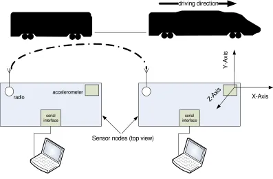
During the first actual data measurement, some shortcomings of the data logger were discovered. The datasets are therefore divided into three sets, each newer sets solves the shortcomings of the previous set. Each dataset consists of the measurements of two nodes (figure 2.4). These nodes are placed in two different wagons behind the same train. Besides the described datasets the aforementioned reference set for verification with two nodes on the same wagon is also recorded, but not further described. Each node is mounted in the same direction where the x-axis represents the driving direction, the y-axis records the sideways movement and the z-axis points downwards. The nodes are mounted by hand so the axes are not aligned perfectly.

Figure 2.4: Test setup two nodes in a train

2.5.1 Dataset 1

The analysis of the first dataset showed a major problem: one of the sensor nodes suffered from radio interference. The disturbance on the radio was not triggered in the faculty building, despite the presence of multiple devices operating in various frequency bands i.e. mobile phones, wireless lan, similar sensor nodes etc. Since the nodes were equipped with a copper wire as antenna it is possible that variations in the wire length are responsible for higher

interference levels on one of the nodes. Besides that, it is also possible that the casing the nodes are mounted in have influence on the radio interference levels, since different cases are used for the nodes. The last possible explanation is the location in the train e.g. radio devices located near the position of one of the nodes.

The interference on the radio stops the logging of the data from the accelerometer, thus the recording of the dataset fails. The accelerometer triggers an interrupt when it has new data only when the previous data has been read out successfully. The radio interference caused the sensor node to miss this interrupt, creating a deadlock situation.

Z-Ax is

Y

-A

x

is

X-Axis

radio accelerometer

serial interface

serial interface driving direction

16 Data Collection

2.5.2 Dataset 2

The software running on the sensor nodes received an update, which addressed the radio interference as well as the deadlock situation, for the measurement of dataset 2. The software part responsible for the radio communication is set to discriminate between radio packets of the system and all other radio data and ignoring the latter completely. Besides that, after the reception and handling of radio data, an additional check of new accelerometer data is performed. The extra check of new accelerometer data ensures that new data is read out even when the interrupt generated by the accelerometer is missed due to handling of radio data. Although the results of the second measurement still showed radio interference on one of the nodes, the node was now able to produce a useful dataset.

2.5.3 Dataset 3

The third dataset is recorded on the same track as dataset 2, giving the characteristics of two trains operating on the same track. Analysis of the second dataset showed that the acceleration levels of the wagons are never above 1g, for all axis. Before starting the third measurement, the range of the minimum and maximum acceleration levels of the accelerometer has been lowered from ±6g to ±2g. This increased the resolution of the measurements.

2.6

Verification datasets

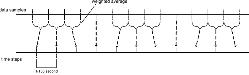
The first software tool written for the analysis of the datasets a tool, checks the number of measurement points between two timestamps. Since the sample rate is set at 160Hz, one would expect 320 sample points between two timestamps, unfortunately one of the nodes showed a lower number of 314 samples per two seconds. The accelerometers have been switched between the µNodes to ensure this could be attributed to the internal clock of the accelerometer, which proved to be a correct assumption.

Since one of the nodes from dataset 1 suffered from radio interference, which caused the node to stop recording data, it is imperative to make sure the device did record enough data samples between two timestamps. Dataset 2 as well as dataset 3 did show some missing timestamps due to the radio interference, but when calculating the average number of samples between the timestamps that did get recorded, it showed no loss of data samples. For example when timestamp 3 is lost, if the average number of data samples between timestamp 2 and 4 still equals the average number of data samples between two sequential timestamps, the recording of the dataset is still considered to be successful.

Figure 2.5: Re-sampling of the data sets

01:00 - 02:00 2:00-03:000 03:004-00:0 06:00-07:00 80:00-0:070 08:00 - 09:00 -102:00:011 12:00 - 13:00 13:00-14:00

data samples

01:00 - 02:00 1/155 second

time steps

18

Chapter Three

Data Analysis

After gathering and verifying the data sets that represent train and wagon movement accurately, the data is analyzed in Matlab. The goal of the data analysis is the discovery of means to discriminate between two wagons behind the same train and all other variations.

3.1

Raw data

Considering the almost unlimited ways of finding patterns in the raw data, the data is first examined more closely. The first step is to look at the raw output of the accelerometers. When combining the data with the known path the wagons have taken a preliminary outcome for the possible ways of correlating the wagons is established. Further analysis by examining the frequency spectrum of the measured signals gives insight in the interesting frequency bands in the signal with regard to the correlation.

3.1.1 Output accelerometers

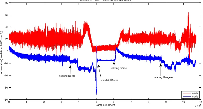
An impression of the measured data is displayed in figures 3.1, 3.2 and 3.3. The displayed data is the raw data obtained for dataset 3 measured in the front wagon. The train has already gained maximum acceleration at the time the measurement started. Approximately halfway, the train arrives at Borne station, thus braking and eventually stopping. After a short stop, the train starts moving towards Hengelo station. Whilst nearing Hengelo station, the train performs a couple of track changes, during which the train starts braking as well. The measurement is stopped a few seconds before the train actually stands still.

Figure 3.1: Raw data x and y axes dataset 3

The raw data of the x-axis in figure 3.1 clearly shows the train gaining speed, braking, pausing and gaining speed again. The difference between the relative straight forward track between Almelo de Riet and Borne and the track changes and curved tracks when nearing Hengelo is also visible.

0 1 2 3 4 5 6 7 8 9 10 11

x 104

-80 -60 -40 -20 0 20 40 60 80

Dataset 3: X and Y axes. Samplerate 155Hz

The sideways movement of the moving train can be distinguished in the data of the y-axis. When the train is standing still at Borne, the amplitude of the y-axis signal is smaller than when the train is moving. When the train is making track changes at the end of the measurement when nearing Hengelo station, the amplitude of the signal on the y-axis increases as well.

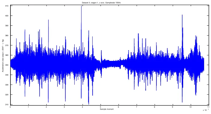
Figure 3.2: Raw data z-axis dataset 3

The raw data of the z-axis, figure 3.2, allows a visible discrimination between driving and standing still. To compensate the lack of correct alignment of the three axes on the different wagons, it is possible to use the magnitude of the three axes. Results in [18] show the possibility of using the magnitude on µNodes as well. Figure 3.3 shows the magnitude of the raw data of the three axes. Since the data of the z-axis contains the largest amplitudes and highest acceleration levels, the magnitude of the three axis shows great similarities to the raw data of the z-axis.

Figure 3.3: Magnitude of raw data three axes

0 1 2 3 4 5 6 7 8 9 10 11

x 104 310 320 330 340 350 360 370 380 390 400 410 Sample moment A cc e le ra ti o n ( ra w o u tp u t + -2 0 4 7 ~ + - 6 g )

Dataset 3, wagon 1, z-axis. Samplerate 155Hz

0 1 2 3 4 5 6 7 8 9 10 11

x 104

300 320 340 360 380 400 420

Dataset 3, wagon 1. Magnitude XYZ-axes. Samplerate 155Hz

20 Data Analysis

3.1.2 Frequency spectrum

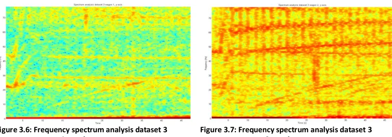
By analyzing and comparing the frequency spectrum of the measured signals, it is possible to discover similarities between two wagons behind the same train. Figures 3.4-3.11 show the result of frequency spectrum analysis of relative small subsets of the datasets. The chosen subsets all start when a train starts leaving station Borne, taken from dataset 3. The subsets are analyzed using a window size of 256 samples with an overlap of 250 samples and a 256 point FFT. The Shannon/Nyquist rule states only frequencies up to half of the sampling rate can be reconstructed, thus the resulting frequency spectrum ranges from 0 to ~ 77 Hz considering the sampling rate of 155Hz of all the measurements.

Figure 3.4: Frequency spectrum analysis dataset 3 wagon 1, x-axis

Figure 3.5: Frequency spectrum analysis dataset 3 wagon 2, x-axis

The frequency spectrum analysis of the x-axis, figures 3.4 and 3.5, show very low frequency components. Since the x-axis is not calibrated to output 0 when the train is in a steady state, the offset it has results in the strong presence of the zero frequency when making a FFT analysis. The measured low acceleration levels indicate that there are possibly other low frequency components in the signal besides the zero element. The frequency spectrum analysis shows activity in the 0 to approximately 2 Hz range, which follows the previous theory. Based on these results correlating the signal after applying a low pass filter is a possible means of relating two wagons.

The higher frequencies also show a pattern in the spectrum analysis, but the pattern is visible in different frequency ranges for each of the wagons, thus correlating the wagons based on other frequencies then the aforementioned low frequencies is highly unlikely.

Figure 3.6: Frequency spectrum analysis dataset 3 wagon 1, y-axis

Figures 3.6 and 3.7 also display strong low frequency components in both the signals.The y-axis is not calibrated to output 0 as well, thus the zero frequency is present due to the standard offset. Besides that, high frequency components are also visible, especially in the frequency spectrum analysis of wagon 2. The visible patterns in red for wagon 2 are present in yellow in the spectrum analysis of wagon 1, but unfortunately these patterns are also shifted in frequency range, as was seen on the analysis of the x-axis. Therefore, the focus for correlation on the y-axis also lies on the lower frequency components.

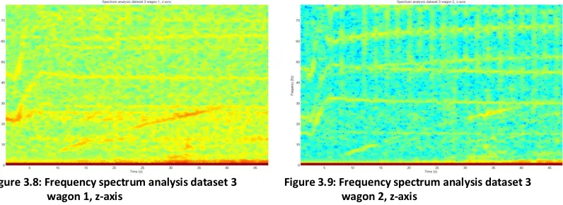
Figure 3.8: Frequency spectrum analysis dataset 3 wagon 1, z-axis

Figure 3.9: Frequency spectrum analysis dataset 3 wagon 2, z-axis

The frequency spectrum analysis of the measurement data of the z-axes, show similar results as seen on the analysis of the x- and y-axes. The lower frequencies are also of more interest for the correlation of two wagons. The frequency spectrum analysis of the magnitude of the three axis again displays the strong presence of low frequency components, whereas the presence of the higher frequency components is shifted when comparing one wagon to another.

Figure 3.10: Frequency spectrum analysis dataset 3 wagon 1, magnitude xyz axes

Figure 3.11: Frequency spectrum analysis dataset 3 wagon 2, magnitude xyz axes

3.2

Correlation filtered data

22 Data Analysis

Figure 3.12: Magnitude (dB) and phase response 2nd order

lowpass Butterworth filter

Figure 3.13: Raw data x-axes accelerating wagons

Figure 3.14 shows the filtered data of the x-axes of three accelerating wagons. Two of these wagons are behind the same train. The dataset of the other train is measured on the same part of track. It is clear to see that the upper and lower graphs belong to the wagons behind the same train. The data of the third wagon does show great similarities when compared to the wagons behind the other train. The main difference between the two trains is the duration of the maximum acceleration before the train has gained speed and gradually lowers the

acceleration levels and the roll-off between the moment of standstill and the point at which the train start accelerating.

The datasets of the wagons behind the same train are identical with regard to duration of the maximum acceleration levels and the roll-off between standstill and the start of the

acceleration. When the train has gained speed and the acceleration levels start dropping gradually, the wagons still show an acceleration level which is on average the same, but both wagons experience peak levels that are unique for each wagon.

Figure 3.14: Data x-axes accelerating wagons, lowpass filtered at 2Hz

The results of the correlation of the filtered datasets is shown in figures 3.15 and 3.16. The data is filtered at 10, 5 and 2 Hz. For reference the original unfiltered data has also been correlated. The chosen correlation window is 5 seconds, 755 samples. When choosing the window size, we have to choose between having a fast response time (small window size) or a more accurate correlation value (large window size). In the next sections, we will motivate our choice of a correlation window of 5 seconds.

0 10 20 30 40 50 60 70 -100 -90 -80 -70 -60 -50 -40 -30 -20 -10 0 Frequency (Hz) M a g n itu d e ( d B )

Magnitude (dB) and Phase Responses

-3.0534 -2.7509 -2.4484 -2.1459 -1.8434 -1.5409 -1.2384 -0.9359 -0.6334 -0.3309 -0.0284 P h a se ( ra d ia n s) Magnitude Phase

0 1000 2000 3000 4000 5000 6000 7000 -20 -10 0 10 20 30 40 Sample moment A cc e le ra ti o n ( + - 2 0 4 7 ~ + - 6 g )

Acceleration on x-axis. 2 Wagons behind 1 train, 1 wagon different train. Both trains same track. Raw data. dataset 3: wagon 2 dataset 2: wagon 1 dataset 3: wagon 1

0 1000 2000 3000 4000 5000 6000 7000

-20 -10 0 10 20 30 40 Sample moment A c c e le ra ti o n ( + - 2 0 4 7 ~ + - 6 g )

Acceleration on x-axis. 2 Wagons behind 1 train, 1 wagon different train. Both trains same track. Data low pass filtered at 2Hz.

Figure 3.15: Correlation lowpass filtered data x-axes two wagons behind same train

Figure 3.16: Correlation lowpass filtered data x-axes two wagons behind different trains

When comparing the different frequencies at which the low-pass filter is set, the lowest setting, 2Hz, results in the best distinction between high correlation, value 1, and no correlation, value 0. Unfortunately, the wagons behind two accelerating different trains display high

correlation during a large window. A possible explanation for this phenomenon is that the used parts of the datasets involve the same part of the track and the same type of trains, which follow the same train schedule, thus the trains show very similar behavior. On the other hand, at the point where the trains perform the highest acceleration, which is the most crucial point of the ride, since it is the starting point at the station, a clear distinction between the two trains is observed.

0 1000 2000 3000 4000 5000 6000

-1 -0.8 -0.6 -0.4 -0.2 0 0.2 0.4 0.6 0.8 1 Sample moment C o rr e la ti o n

Correlation on x-axis. Correlation window: 5s. Samplerate 155Hz 2 wagons behind accelerating train.

unfiltered L10 L5 L2

0 1000 2000 3000 4000 5000 6000

-1 -0.8 -0.6 -0.4 -0.2 0 0.2 0.4 0.6 0.8 1 Sample moment C o rr e la ti o n

Correlation on x-axis. Correlation window: 5s. Samplerate 155Hz 2 wagons behind accelerating different trains.

24 Data Analysis

Figures 3.17, 3.18 and 3.19 show the correlation of the low-pass filtered data of two wagons in three different situations with increasing correlating window sizes.

Figure 3.17: Correlation with varying window sizes. Two wagons behind same accelerating train

Figure 3.18: Correlation with varying window sizes. Two wagons behind accelerating different trains

The results in figures 3.17 and 3.18 suggest a correlation window of 455 samples, 3 seconds, already provides a sufficient distinction between intended correlation and coinciding

correlation. When taking the varying correlation window sizes applied to two completely different wagons, figure 3.19, into account it is clear that the correlation window size should be at least 620 samples, 4 seconds, but preferably 775 samples, 5 seconds. With a window size of 775 samples, the correlation between an accelerating wagon and a stationary wagon is close to zero thus giving a relatively large distinction between related wagons and non-related wagons.

0 1000 2000 3000 4000 5000 6000 7000

-1 0 1

Correlation using varying window sizes. Axis: x. Low-pass filtered at 2Hz Wagons: 2 wagons behind accelerating train.

155

0 1000 2000 3000 4000 5000 6000 7000

-1 0 1 310

0 1000 2000 3000 4000 5000 6000 7000

-1 0 1 465

0 1000 2000 3000 4000 5000 6000 7000

-1 0 1 620

0 1000 2000 3000 4000 5000 6000 7000

-1 0 1 775

0 1000 2000 3000 4000 5000 6000 7000

-1 0 1

Correlation using varying window sizes. Axis: x. Low-pass filtered at 2Hz Wagons: 2 wagons behind accelerating different trains.

155

0 1000 2000 3000 4000 5000 6000 7000

-1 0 1 310

0 1000 2000 3000 4000 5000 6000 7000

-1 0 1 465

0 1000 2000 3000 4000 5000 6000 7000

-1 0 1 620

0 1000 2000 3000 4000 5000 6000 7000

Figure 3.19: Correlation with varying window sizes. One accelerating wagon, one stationary wagon

Figure 3.20: Correlation two wagons behind accelerating train, y-, z- and xyz-axes

Figures 3.20, 3.21 and 3.22 display the correlation of the other axes, including the correlation of the magnitude of three axes. The correlation of the z-axis and the magnitude of the axes are too low in the case of the two wagons behind the same train, figure 3.20, to be the only factor to rely on for the discovery of the train composition. When taking the correlation of two wagons behind two accelerating different trains also into account, figure 3.21, during the department of the station no reliable distinction between two trains can be established. The correlation of the data of the y-axes shows a similar pattern as the correlation of the data of the x-axes when comparing the results of two wagons behind the same train and the two wagons behind accelerating different trains, but when the train starts accelerating the correlation level of the two wagons behind the same train is lower for the data of the y-axes than for the data of the x-axes. This renders the correlation based on the data of the y-axes less usable than correlation based on the data of the x-axes.

0 1000 2000 3000 4000 5000 6000 7000

-1 0 1

Correlation using varying window sizes. Axis: x. Low-pass filtered at 2Hz Wagons: 1 wagon behind accelerating train, 1 wagon behind stationary train .

155

0 1000 2000 3000 4000 5000 6000 7000

-1 0 1 310

0 1000 2000 3000 4000 5000 6000 7000

-1 0 1 465

0 1000 2000 3000 4000 5000 6000 7000

-1 0 1 620

0 1000 2000 3000 4000 5000 6000 7000

-1 0 1 775

0 1000 2000 3000 4000 5000 6000

-1 0 1

sample moment y

Correlation on y-,z- and xyz-axes. Correlation window: 5s. Samplerate 155Hz 2 wagons behind accelerating train.

unfiltered L10 L5 L2

0 1000 2000 3000 4000 5000 6000

-1 0 1

sample moment z

0 1000 2000 3000 4000 5000 6000

-1 0 1

26 Data Analysis

Besides that, when comparing the correlation around the 1000 sample point mark, the two wagons behind the two accelerating different trains start correlating again in contrary to the two wagons behind the same train, which indicates the y-axis is an unreliable source for correlation.

Figure 3.21: Correlation two wagons behind accelerating different trains, y-, z- and xyz-axes

Figure 3.22: Correlation one accelerating wagon and one stationary wagon, y-, z- and xyz-axes

Since only the lower frequencies contain useful information, a lower sample rate should be sufficient for the correlation analysis as well. Figures 3.23 and 3.24 show the correlation of the datasets when re-sampled at 35Hz using the method described in section 2.6. When comparing these figures with figures 3.15 and 3.16 it is clear that datasets recorded at a sample rate of 35Hz produce the same correlation result as datasets recorded at higher sample rates.

0 1000 2000 3000 4000 5000 6000

-1 0 1

sample moment y

Correlation on y-,z- and xyz-axes. Correlation window: 5s. Samplerate 155Hz 2 wagons behind accelerating different trains.

unfiltered L10 L5 L2

0 1000 2000 3000 4000 5000 6000

-1 0 1

sample moment z

0 1000 2000 3000 4000 5000 6000

-1 0 1

sample moment xyz

0 1000 2000 3000 4000 5000 6000

-1 0 1

sample moment y

Correlation on y-,z- and xyz-axes. Correlation window: 5s. Samplerate 155Hz 1 wagon behind accelerating train, 1 wagon behind stationary train .

unfiltered L10 L5 L2

0 1000 2000 3000 4000 5000 6000

-1 0 1

sample moment z

0 1000 2000 3000 4000 5000 6000

-1 0 1

Figure 3.23: Correlation two wagons behind accelerating train, data resampled at 35Hz

Figure 3.24: Correlation two wagons behind accelerating different trains, data resampled at 35Hz

0 500 1000 1500

-1 -0.8 -0.6 -0.4 -0.2 0 0.2 0.4 0.6 0.8 1

Sample moment

C

o

rr

e

la

ti

o

n

Correlation on x-axis. Correlation window: 5s. Samplerate 35Hz 2 wagons behind accelerating train.

unfiltered L10 L5 L2

0 500 1000 1500

-1 -0.8 -0.6 -0.4 -0.2 0 0.2 0.4 0.6 0.8 1

Sample moment

C

o

rr

e

la

ti

o

n

Correlation on x-axis. Correlation window: 5s. Samplerate 35Hz 2 wagons behind accelerating different trains.

28 Data Analysis

3.3

Conclusions

The results of the data analysis show that a distinction between two wagons behind the same train and two unrelated wagons can be made based on the correlation of the acceleration levels of the wagons in the driving direction of the train. The high frequency components of the acceleration data contain too much noise to be useful for correlation. A spectrum analysis does show similar patterns between two related wagons in the higher frequencies, but unfortunately these patterns occur in different frequency bands for each of the wagons, rendering a

correlation based on these patterns impractical. The low frequency spectrum proved useful for the correlation. When low-pass filtering the acceleration data of the driving direction at 2Hz two wagons behind the same train can be distinguished. The amount of time the distinction is evident is relatively small when two wagons behind the same train are compared to a wagon behind another train, which drives on the exact same location using approximately the same amount of acceleration.

Although there exists a small window in which the distinction is made, it should be noted that this window is very small under rare conditions. Using the acceleration data of the driving direction of the wagons for simulations is considered the best option based upon two

observations. First of all it is highly unlikely that two trains depart at the exact same time with a near identical amount of acceleration. The circumstances under which the acceleration data is recorded for data analysis were artificial. The trains in which the data is recorded were all of the same build sporting the same train composition. Besides that, the recorded data is synchronized before performing a correlation analysis. Thus, having a synchronous departure combined with different train characteristics and the amount of acceleration provided by the driver leading to similar acceleration levels seems unlikely in practice.

Secondly, when using wireless sensor nodes, two trains will usually be out of radio range within a short amount of time after departing a shunting yard or station, which renders the fact that these two trains perform the same operation at the same time insignificant. Combining these two facts results in a very low possibility only a small distinction window is available. Simulations will prove if the small window is a problem to reckon with.

The correlation of the acceleration levels of the other axes also showed high levels of

29

Train Composition Algorithm

In the previous chapter, we prove our assumption, that we can distinguish trains from each other using movement as common context, is valid. The next step in our research is constructing a train composition algorithm based on our assumption and the results of our data analysis. The discovery of the train composition is divided in three steps. In this chapter, we describe how we implemented these steps in our algorithm. Our research lays the emphasis on the second step of the process, the correlation. For the first and the last step, we provide possible

implementations.

4.1

Pairing

The train composition algorithm works in a distributed fashion. A pair of two sensor nodes calculates their correlation on which the locomotive will eventually base the train composition. In the following two sections, we describe the initialization and operational phases.

4.1.1 Wake-up

As soon as a node detects movement, the node wakes up. For this a ball-switch [8], [20] can be used. We assume all nodes behind the same locomotive are able to detect initial movement of the locomotive and are able to wake-up within a certain relatively small time window. When a node has detected the movement and the node is in an active state, the node starts the network interface and announces its presence to other nodes using a broadcast on the network. Nodes that are also still in the first step of the process can respond to this broadcast message upon reception. When two nodes have acknowledged their existence, these nodes form a pair.

Nodes that did not respond to the broadcast message are either not within radio range or on a different train. Based on our assumption that nodes are able to wake-up within a certain time window after the initial movement of the locomotive, the window for sending and

acknowledging a broadcast message can be set at a fraction larger than the maximum time a node requires for waking up after the locomotive starts moving. The trains we used for the recording of our datasets showed only very small, less than 5 ms, delay in the detection of train movement, but depending on the type of connection between wagons this number may vary.

4.1.2 Master/slave

Nodes forming a pair exchange data from their accelerometers to be able to decide if these two nodes are behind the same locomotive or not. Based on our conclusions from chapter three, the data of the axes measuring the driving direction is used. The data is sampled at 35Hz and filtered using a low-pass filter at 2Hz.

30 Train Composition Algorithm

For reduction of overhead each network packet instigates, we propose to send data from slave to master in a bulk packet containing the last 35 samples. The downside of this approach is the fact that the rate, at which we can draw conclusions based on the outcome of our correlation calculations, is also limited to one per second. Simulation results will show this will not limit our ability to detect the train composition in an early stage after the train starts accelerating.

4.2

Correlation

4.2.1 Correlation algorithm

We implement the correlation of two nodes using the Pearson product-moment correlation coefficient ρX,Y , which can be found in equation (1). For the implementation of the calculation of this correlation coefficient, let x and y be two sensors nodes on a train, that have established a

master/slave relation. Our window size is represented as n. The data send between each master

and slave, is represented by xj and yj with j=1 for the oldest data point recorded by both nodes.

, ,

(1)

1

(2)

, 1

(3)

As can be seen in equations (1), (2) and (3) a straightforward implementation requires a relatively large amount of computations on each pair of nodes for computing the correlation coefficient upon reception of the data from the slave.

Marin-Perianu et al. [7] propose an optimization to the correlation calculation algorithm. The proposed algorithm stores intermediate values thus reducing the amount of calculations necessary for the computation of each correlation coefficient. Equations (4)-(13) show which steps are taken for the calculation of the correlation coefficient as well as the intermediate values. In our algorithm, k is fixed at 35 and n=k*m thus m depends on window size n. When the window size is n, the optimized algorithm requires the availability of the last m intermediate values, thus the number of intermediate values stored by both the master and slave relates to the largest window size used in our algorithm. Each calculation of the correlation coefficient is referenced by i, which starts at 1. The intermediate values we calculate and use are calculated using the following equations:

!

(4)

"

!

!

(6)

"

!

(7)

"

! (8)

$ # % #

&

(9)

$ # % # "

&"

(10)

The variance and covariance calculations using the intermediate values are performed as follows:

()

() % &

# #

(11)

()

() %" &"

# #

(12)

,

, %*+,- *+./

$ #$ #

# #

(13)

32 Train Composition Algorithm

4.2.2 Window size

Based on our conclusions in chapter three, for determining if two nodes are behind the same train, a correlation window of 3 seconds (105 samples) is sufficient for the detection of two wagons behind the same train. On the other hand, a window smaller than 5 seconds (175 samples) leads to false positives, i.e. nodes behind different trains assume they are behind the same train. The disadvantage of the correlation window is the delay with which the final train composition is deduced, thus a smaller window size is preferred.

To facilitate a window of 3 seconds as well as a window of 5 seconds, our algorithm is able to calculate the correlation of two nodes over a growing window. The disadvantage of this approach is the inability to use the optimization as proposed by Marin-Perianu et al. [7] while the correlation window is still growing. Our algorithm starts the decision process when the window size has reached 3 seconds. Although this leads to false positives, our data analysis has shown no false negatives, thus the algorithm is already able to eliminate nodes not behind the same train. The elimination of non-correlating nodes in an early stage of the algorithm offers improved energy efficiency. The fact that non-correlating nodes are eliminated in an early stage and the fact that the number of computations needed for smaller windows is less, compensate for the lack of optimization of the calculation of the correlation coefficient.

4.3

Train composition

Our algorithm is limited to the correlation of the node pairs. For the discovery of the train composition we identify two scenarios. Results from our simulation will give a good estimation for the point in time at which we are able to deduce the actual train composition i.e. when all nodes behind the same train are correlating and there is no correlation between nodes from different trains. After the train composition is determined, we propose to send a message to all nodes, which the nodes should acknowledge to verify that they are still behind the locomotive thus the train integrity is still guaranteed.

In the other scenario, we assume we are able to identify the last wagon of the train. For example by implementing a RFID system on each node with which a person can generate an interrupt signaling the node is on the last wagon. After the correlation phase has ended, the last node sends a route discovery message towards the locomotive. Using this approach, the locomotive is able to deduce a better estimate of the train composition i.e. instead of a tree view of the wagons, the locomotive is able to view the wagons as a straight line. Besides that, the communication necessary for the train integrity message involves fewer nodes, since the start and end nodes of the train are known and the train integrity is still intact as long as the last wagon can be reached. This leads to a reduction in network traffic and improves energy

efficiency. The discovery of the route to the locomotive can be implemented using existing algorithms e.g. AODV [21] or ODMRP [22].

34

Chapter Five

Simulation

5.1

Network

The following sections describe the link connectivity model we used and the assumptions we made for the network communication in our simulation.

5.1.1 LogNormal Shadowing

Since the environment the wireless sensor nodes are operating in contains large objects, using a circular radio model would give a distorted image of the actual network performance of the sensor nodes. We therefore implement the LogNormal Shadowing (LNS) model [23] in our simulation. The concept behind the model is that statistical variations of the radio signal power around its mean value are taken into account when calculating the link probability. The LNS model enables us to calculate the link probability between two nodes given the normalized distance between two nodes and parameter ξ. The parameter ξ controls the influence of variations in signal power on the link probability, thus enabling us to simulate for example a shunting yard with a large amount of large objects. Figures 5.1 and 5.2 show the connectivity and communication range of node A when using either a circular radio model or the LNS model.

Figure 5.1: Circular radio model Figure 5.2: LogNormal Shadowing model

The LogNormal Shadowing model calculates the link probability using equations (14) and (15). Parameter ξ is defined as the ratio between the standard deviation of shadowing (σ) and the pathloss exponent (n). The parameter ξ can vary between 0 and 6 where a value of 0 gives the same link probability as a circular radio model and a value of 6 equals heavy shadowing. Variable

)̂ represents the normalized distance between two nodes and α is a constant with value:

1 )̂ 1_{2 31 4)5 67}89 )̂_{: ;<} (14)

: = ⁄ (15)

5.1.2 Acknowledgment and retransmission

Considering the safety requirements on the train composition algorithm we use a MAC layer model that requires each message sent to be acknowledged. Each message that is sent between nodes is tagged with a priority. The priority of a message is a number which resembles the number of retries we perform at maximum when sending the message or the corresponding acknowledgement before we consider the transmission of the message failed. Table 5.1 gives an overview of the used priorities.

Priority Retries

PRIORITY_BROADCAST 1

PRIORITY_LOW 2

PRIORITY_MEDIUM 3

PRIORITY_HIGH 5

Table 5.1: Relation between priorities and number of retries

Using the link probability we have calculated between nodes using the LSN model, we decide whether a packet has reached its destination or not. Besides point-to-point messages, we assume nodes are also able to send a broadcast message. This broadcast message is for example used to discover master/slave pairs. The broadcast message uses the same methods as the point-to-point messages, but with a priority of 1, thus a broadcast message is either received and acknowledged directly or not.

The exchange of the correlation data messages uses the low, medium and high priorities to send the messages as follows: the correlation data is initially send with priority low, when the data exchange fails, a higher priority is used. When a higher priority is selected, all further correlation interaction will also use this higher priority. In case the data exchange fails at the highest priority, the nodes stop interacting and lose their master/slave status. During one correlation step, i.e. the exchange of data points and the calculation of the correlation, it is possible that data exchange is retried at a higher priority.

5.1.3 Packet size

36 Simulation

The size of a packet is expressed in bytes. In some cases, this will introduce a small overhead for each packet, since not all bits of every byte might be needed. We choose this approach because an implementation of the train composition algorithm on nodes using an existing network layer forces the use of predefined packet formats, which usually do not allow packet sizes to be trimmed to the exact amount of bits necessary. Table 5.2 gives an overview of the packets and the corresponding sizes we use.

Packet type Packet size (bytes)

Broadcast 3

Acknowledgement 3

Data points 89

Correlation result 29

Table 5.2: packets and corresponding sizes

We assume each node requires two bytes for a unique ID, which functions as the destination address. Besides that, each packet has one byte that we use for the definition of the type of packet. The packet with data points includes the mean, sum, sum of squares and variance of the set. The correlation result packet includes the mean, sum, sum of squares, variance of the master node as well as the sum of products, covariance and correlation of both sets. The results of the calculations are stored in 32 bits, 4 bytes, except for the correlation, which is stored in 16 bits, 2bytes.

As soon as the correlation window has reached the maximum size and the algorithm switches to the optimized correlation algorithm, the slave no longer needs to calculate the variance of its data points, thus the packet size of the data points reduces with 2 bytes.

Using the numbers from table 5.2 the total number of bytes required for a correlation cycle is 124 bytes, consisting of two acknowledgements, a set of data points and the correlation result.

5.2

Train and nodes

In the following sections, we explain how the nodes and trains are setup in our simulation.

5.2.1 Train and node layout

Our simulation is based on several locomotives with a number of freight wagons behind them. For the measurements of the locomotives and freight wagons we used the average length and width as seen on Dutch freight trains [24] i.e. a length of 20m and a width of 3m. On each side of a train, we reserve 1m of clearance space. For an even distribution of nodes on the wagons and train, we place two nodes on each wagon or train, which are located at the long-sides in the middle as shown in figure 5.3. By placing the nodes on the long side of the wagons, nodes on the same side are able to communicate in a less obstructed way. When placing nodes on the short sides, nodes on two adjacent wagons are either within very short range or at least one of the wagons is blocking a direct path between two nodes, both situations have a negative impact on the radio communication.

Figure 5.3: Sensor node placement on freight train wagon

5.2.2 Train movement

The data we use for correlation is also used for determining the speed of a train by integrating the acceleration. Besides the speed of the train, we can also adjust the direction in which the train travels, which is either to the left of the shunting yard or to the right.

5.2.3 Shunting yard

As stated in our preliminary research, the worst-case scenario contains multiple trains departing at the same time within radio range of each other. Our simulation is based on this worst-case scenario. On our shunting yard, we position multiple trains. The wagons of a train are always behind the locomotive, thus the driving direction of the train is determined before we place the train. We either pick a random direction for each train or each train drives in the same direction. The locomotives of the trains are positioned either on the left half of the yard or on the right half of the yard. When a train drives to the left, we always place the locomotive of the train in the right half of the shunting yard and vice versa, this ensures wagons of all trains are situated within the center area of the shunting yard before all trains start accelerating. An example of the positioning of the trains is given in figure 5.4.

Figure 5.4: Positions of trains on shunting yard

38 Simulation

5.3

Results

In order to answer our research questions we recorded several statistics during each run of the simulation. The statistics we recorded are:

• Time at which the composition of all trains can be correctly determined

• Number of master roles a node fulfills and the time at which this occurs

• Number of slave roles a node fulfills and the time at which this occurs

• Network statistics e.g. number of bytes sent and received, number of packets sent and

received

Each simulation run is configured using the possibilities described in the previous section. We varied the following settings:

• Number of trains

• Positioning of trains

• Driving direction

• Delay between the departure of one train and the departure of the next train

We simulated each different setting 100 times.

5.3.1 Correlation

In table 5.3, we present a summary of the results on the accuracy of the train composition determination. The first four columns show the settings for the simulation runs i.e. the number of trains, the positioning of the trains, the driving directions and the delay between the departures of the trains. The following column shows the failure rate. We identify two possible ways the distributed algorithm has failed, when within 15 seconds:

• Wagons behind different trains are still correlating

• It is not possible to reach all wagons behind the same train using the tree formed by all correlating pairs

Trains Position Direction Delay (samples)

Failure Min

(samples) Max (samples) Avg (samples) Std (samples)

2 - - - 0% 70 70 70 0

3 Fixed fixed 15 0% 280 280 280 0

3 Fixed fixed 20 0% 280 280 280 0

3 Fixed fixed 30 0% 245 245 245 0

3 Fixed random 15 0% 280 280 280 0

3 Fixed random 20 0% 280 280 280 0

3 Fixed random 30 0% 245 245 245 0

3 random fixed 15 0% 70 280 214,12 96,80

3 random fixed 20 0% 70 280 224,41 93,10

3 random fixed 30 0.98% 70 245 196,96 78,48

3 random random 15 0% 70 280 180,15 104,87

3 random random 20 0% 70 280 171,23 86,84

3 random random 30 0% 70 245 151,15 97,92

Table 5.3: Results correlation calculations using different settings

For the simulation of the two trains we used two datasets with different characteristics. In figures 5.5 and 5.6 we can clearly see one of the trains reducing its acceleration levels, the distinction between these two trains using our correlation algorithm is therefore made in an early stage of the simulation. For all different settings, the outcome for the situation with two trains remained the same; therefore, only one entry is found in table 5.3 for this situation. The results of the simulation with the two trains indicate it is possible to determine the train compositions after 70 samples, 2 seconds.

Figure 5.5: Train accelerating fully after departure

Figure 5.6: Train not accelerating fully after departure

The datasets used in the situation with three trains, contain two sets with very similar characteristics. Using the different settings, we measured different results in the situation with three trains, therefore we include the summary of all different settings for this situation in table 5.3. We observe a low failure rate of 0.98% in one setting. Since we did not register any failures in all other cases, we describe this particular failure to reoccurring packet loss.

0 100 200 300 400 500 600 700 800 900 1000 0 5 10 15 20 25 30 Samples A c c e le ra tio n le v e l

Acceleration levels of train. Dataset 2, second departure. Low-pass filtered at 2Hz

0 100 200 300 400 500 600 700 800 900 1000 0 5 10 15 20 25

Acceleration levels of train. Dataset 2, third departure. Low-pass filtered at 2Hz

40 Simulation

The correlation for the two subsets with similar characteristics is more difficult and results in more samples needed before the discovery of the correct train composition. The minimum and maximum amount of samples needed for the correct discovery of the train compositions, show a relatively large difference when compared to the situation with the two trains and looking at the settings where at least one setting is set at random. As long as the trains are driving side by side in the same direction, no difference between the minimum and maximum amount of samples is visible.

We observe the maximum number of samples required is lower when the delay between the depa