An Analysis of the Effects of Digital
Phase Errors on the Performance of a
FMCW-Doppler Radar
by
Kurt Peek
Picture: www.thalesgroup.com
A thesis submitted in partial fulfillment
Of the requirements for the degree of
MASTER OF SCIENCE in APPLIED PHYSICS
at
The University of Twente
2
Abstract
3
Table of Contents
1 Introduction ... 4
1.1 Linear frequency-modulated continuous-wave radar ... 5
1.2 Frequency sweep linearity... 9
1.3 Digital chirp synthesis... 11
1.4 This thesis ... 14
2 Theory of operation of a model FMCW-Doppler transceiver ... 15
2.1 Description of the model system ... 15
2.2 FMCW Doppler signal processing ... 17
2.3 Direct digital synthesis ... 33
2.4 Statement of the problem ... 41
3 An analysis of the effect of digital phase errors in the transmit signal on the beat signal spectrum ... 42
3.1 Mathematical model of a FMCW transceiver ... 42
3.2 Model of the phase errors in the digital samples generated by a DDS ... 53
3.3 The effect of periodic digital phase errors on the FMCW transceiver ... 56
3.4 Form of the digital phase error ... 68
3.5 An upper bound for the effect of digital phase errors on the beat signal spectrum ... 72
4 The effect of phase errors on Doppler processing ... 74
4.1 The effect of sinusoidal phase errors in the beat signal ... 74
4.2 The effect of sinusoidal phase errors in the transmitted signal ... 75
4.3 Verification by simulation ... 77
4.5 Conclusion ... 78
5 Implementing periodic and phase-continuous sweep transitions ... 79
5.1 Introduction ... 79
5.2 Chirp DDS discretization constraints ... 82
5.3 Selecting chirp parameters for CP frequency sweeping ... 85
5.4 Algorithm for selecting DDCS parameters ... 87
5.5 Concluding remarks... 90
6 Conclusions and discussion ... 91
6.1 Summary of contributions to knowledge ... 91
6.2 Implications for technological development ... 92
6.3 Recommendations for further research ... 93
4
1
Introduction
“To see and not be seen” has been a cardinal principle of military commanders since the inception of warfare. Until the advent of World War II, the only means available to commanders from this point of view was espionage and intelligence gathering missions behind enemy lines. Just prior to World War II, the allies came up with a groundbreaking invention, the pulsed radar1 which radically changed the equation and for the first time one could see without being seen in true sense of the term.
Figure 1 One of the 60 Chain Home radar sites employed by the Royal Air Force (RAF) during World War II. Three of the four transmitter aerials are visible to the left, while four receiver masts are grouped to the right. (Picture from
http://spitfiresite.com/2010/04/early-radar-memories.html).
The pulsed radar estimates target range by transmitting a sequence of pulses of radio frequency (RF) energy and measuring the time for echoes scattered off the target to return to the radar. One of its earliest embodiments, the Chain Home coastal surveillance system (Figure 1), could sight German fighter formations well before they reached the English coast and could therefore concentrate allied fighter groups where they were most needed. The German fighters were not even aware that they were detected. In effect, the pulsed radar acted as a force multiplier and helped the allies defeat the vastly superior Luftwaffe in the Battle of Britain. The allies pressed home their advantage of having radar by going on the win the Battle of the Atlantic against German U-boats, catching them
unawares on the surface at nighttime when they were charging their batteries. The German reaction to these events was slow and by the time they came up with their own radars and radar emission detectors (now called intercept receivers) it was too little, too late to influence the outcome of the war in their favor (Willis and Griffiths 2007).
After the war, understandably, radar engineers around the world concentrated on developing radar emission detectors (intercept receivers) during the Cold War that followed. This led to a “classic” situation in which intercept receivers had no difficulty detecting radar beams, and sometimes even their sidelobes, at long ranges. This is because the radar signals have to travel to the target and be partially reflected back to the radar, whereas the intercept receiver can intercept them after only a single trip. Since the ‘reflection’ of a radar signal generally involves the target intercepting only a small amount of the transmitted signal and scattering it over a wide volume, the effect is worse than
1
5 just a doubling of the path length: it changes the fall-off in signal strength with range from a square-law process for an intercept receiver to one following a fourth-power square-law for a radar (Skolnik 2008). The intercept receiver does not have things all its own way, however, because the radar has control of its own transmissions, and knows exactly what the received signals should look like, whereas the intercept receiver has only an approximate idea of the radar’s characteristics, and must be general enough to be able to detect a wide variety of different radars. This means that whereas the radar receiver is optimally matched to receive its own transmissions, the ESM receiver is poorly matched to the radar (Fuller 1990).
Low probability of intercept (LPI) radars – which as their name suggests, can be intercepted, but with a low probability – attempt to exploit this advantage by resorting to continuous-wave (CW)
transmissions instead of pulsed transmissions (Figure 2). CW transmissions employ low continuous power instead of the high peak power of pulsed radars, but achieve the same detection
performance. This is possible because it is the average transmitted power that determines a radar’s detection performance (Skolnik 2008).
Figure 2 Illustration of a radar pulse (red) and a continuous-wave radar signal (green).
A “pure” CW radar transmitting continuous power at a single frequency, such as a traffic speed gauge, can only measure shifts in Doppler frequency, and cannot measure the range of targets. In order to measure range, the transmitted signal needs to be imparted a bandwidth – that is, the carrier wave must be modulated.
1.1
Linear frequency-modulated continuous-wave radar
One of the most popular forms of LPI modulation is linear frequency modulation (LFM), in which the instantaneous transmitted frequency is varied linearly with time. The linear variation of frequency with time is commonly referred to as a chirp or frequency sweep. Since the frequency cannot increase indefinitely, the time-frequency characteristic of the waveform is repeated periodically in a sawtooth or triangular fashion to generate a CW signal, as illustrated in Figure 3.
pulse with high peak power
continuous wave with low peak power
6
Figure 3 Schematic of a linear chirp (‘up-chirp’) with period 𝑻, frequency deviation 𝑩, and center frequency 𝒇𝒄.
The frequency sweep effectively places a ‘time stamp’ on the transmitted signal at every instant, and the frequency difference between the transmitted signal and the signal returned from the target (i.e. the reflected or received signal) can be used to provide a measurement of the target range, as illustrated in Figure 4.
time amplitude
frequency
time 𝑓𝑐 = 10 GHz
𝑇 = 400 µs
7
Figure 4 Basic principle of FMCW radar. Top left: time vs. instantaneous frequency plot of a transmitted linear chirp (solid line) with duration 𝑻 and bandwidth 𝑩, and its echo from is a target (dashed line) is received 𝝉 seconds later. The difference or ‘beat’ frequency 𝒇𝒃 between the transmitted and received signals is indicated. Bottom left: the amplitude
of the beat signal with frequency 𝒇𝒃 as a function of time. Bottom right: the spectrum of the beat signal is a ‘sin(x)/x’ or
‘sinc’ function centered at the beat frequency 𝒇𝒃, with a spectral width (strictly, width at -3.9 dB) of 𝟏 𝑻 − 𝝉 , equal
to the reciprocal of the period that the transmitted and received signals overlap in time. For 𝝉 ≪ 𝑻, the target spectral width is approximately 𝟏/𝑻. (After (Willis and Griffiths 2007)).
As seen from Figure 4, the beat frequency 𝑓𝑏 is proportional to the target transit time 𝜏, and thus to
the target range. More precisely, the proportionality constant between the two is the ratio of the chirp bandwidth 𝐵 to the sweep period 𝑇, or chirp rate:
𝑓𝑏
𝜏 =
𝐵
𝑇. (1.1)
For a stationary target, the two-way propagation delay to the target and back, 𝜏, is given by 𝜏 =2𝑅
𝑐 , (1.2)
where 𝑅 is the target range and 𝑐 is the propagation velocity. Combining (1.1) and (1.2) and yields the FMCW equation relating range to beat frequency:
𝑅 = 𝑐𝑇
2𝐵𝑓𝑏. (1.3)
instantaneous frequency
𝑇
𝐵
𝜏
𝑓
𝑏receiver output amplitude
time transmitted
chirp
target echo
frequency
𝑓
𝑏1/𝑓
𝑏time
1
𝑇 − 𝜏
≈
1
𝑇
receiver output spectrum
8 Thus, in FMCW radar, range is proportional to beat frequency2. Hence, by measuring the spectrum of the beat signal, a 1-D down-range map of target radar reflectivity vs. range, called the range profile, can be obtained.
The block diagram of a FMCW transceiver in Figure 5 shows how this is implemented. The beat signal is generated using a mixer3. The local oscillator (LO) port of the mixer is fed by a portion of the transmit signal, while the radio frequency (RF) port is fed by the target echo signal from the receive antenna. The ideal output of the mixer, called the intermediate frequency (IF) signal, is the product of the RF and LO signals, and consists of two components: one at the sum of the RF and LO
frequencies, and one at their difference. The sum-frequency term is an oscillation at twice the carrier frequency of the transmitted chirp, and is filtered out either actively, or more usually because it is beyond the cut-off frequency of the mixer and subsequent receiver components (Brooker 2005). Thus, the signal passed to the spectrum analyzer is at the difference or ‘beat’ frequency as described above. The beat signal is passed to a spectrum analyzer, which is a bank of filters used to resolve targets in to range bins. Typically, the spectrum analyzer is implemented as an analog-to-digital converter (ADC) followed by a processor based on the fast Fourier transform (FFT).
Figure 5 Simplified block diagram of a FMCW transceiver. A continuous-wave (CW) signal is modulated in frequency to produce a series of linear chirps (upper inset), which is radiated towards a target through an antenna. Typical parameters of the transmitted chirps are a carrier frequency of 𝒇𝒄 = 10 GHz, a sweep period of 𝑻 = 500 μs, and a chirp
bandwidth of 𝑩 = 50 MHz. The target echo received 𝝉 seconds later is mixed (multiplied) with a portion of the
transmitted signal, obtained from the transmit path through a directional coupler, and the result is passed to a spectrum analyzer. For a single target, the power spectrum is a sharply peaked ‘sinc’ function (lower inset).
2 Equation (1.3) holds for stationary targets. In the presence of (radial) target motion, the beat frequency 𝑓
𝑏 will be perturbed by a Doppler shift 𝑓𝑑 which, if not compensated, will change the apparent range of the target. This phenomenon is called range-Doppler coupling and is discussed in Chapter 2.
3
A mixer is a three-port device that uses a nonlinear or time-varying element to achieve frequency conversion (Pozar 2005). In its down-conversion configuration, it has two inputs, the radio frequency (RF) signal and the
local oscillator (LO) signal. The output, or intermediate frequency (IF) signal, of an idealized mixer is given by the product of RF and LO signals.
9 The 100% duty cycle of a FMCW radar means that the transmit energy is spread over the whole duration 𝑇, and whole bandwidth 𝐵, of the sweep. However, the beat frequency energy is ‘focused’ into an equivalent bandwidth of 1/𝑇. This allows the FMCW receiver to narrow its noise bandwidth by a factor 𝐵𝑇, the time-bandwidth product of the radar, and thus increase its sensitivity. This in turn allows the transmitted power to be reduced significantly; for example, the Thales Surface Scout radar transmits as little as 10 mW (Thales Nederland 2010). This low power level is very difficult for intercept receivers to detect, which means that FMCW radar can be used in otherwise restrictive emissions control (EMCON) conditions that would preclude the operation of pulsed radar (Pace 2004).
1.2
Frequency sweep linearity
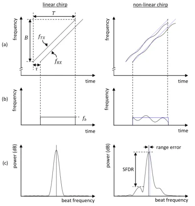
In FMCW radar systems, successful range processing depends critically on the linearity of the FM sweep, or equivalently, on the presence of phase errors in the transmitted signal4. Deviations of the frequency sweep from linearity cause spreading the beat frequency spectrum resulting in degraded range performance as illustrated in Figure 6. Sinusoidal phase errors manifest themselves as
spurious “ghost” targets or “paired echoes” placed symmetrically at both sides of the desired target peak (Griffiths 1991), whereas frequency nonlinearities following a power law lead to biased range estimates as well as spurious (Sheehan and Griffiths 1992). The ratio (in decibels) of the target peak signal to worst-case spurious sidelobe defines the spurious-free dynamic range (SFDR) of the radar.
4 Amplitude errors are also important in principle, but can be removed by operating an amplifier in saturation
10
Figure 6 FMCW operation with linear chirps (left), and a non-linear chirps (right). The blue dashed lines on the right figures reproduce the linear case for ease of comparison. From top to bottom, we show (a) time vs. frequency plots of the transmitted and received signals, denoted 𝒇𝑻𝑿 𝒕 and 𝒇𝑹𝑿 𝒕 respectively; (b) the time vs. frequency plot of the beat
signal; and (c) the power spectrum of the beat signal. The range error and spurious-free dynamic range (SFDR) due to the non-linearity of the sweep are indicated.
The sweep linearity of a FMCW radar depends on how the transmitted signal is generated. In the first commercial FMCW navigation radar, the PILOT (Philips Indetectable Low Output Transceiver) developed by Philips Research Laboratories in 1987, the frequency sweep was generated by driving a YIG-tuned oscillator5 with a linear sawtooth current (Beasley, Leonard et al. 2010) as shown in Figure 7.
5 A YIG (Yttrium, Iron, and Garnet)-tuned oscillator is an oscillators whose frequency varies linearly with the
applied current. At its heart is a YIG sphere which, due to its ferrite properties, resonates at microwave frequencies when immersed in a DC magnetic field. The frequency of resonance increases linearly with the applied magnetic field. A coupling structure, often referred to as the “coupling loop”, is utilized to couple RF energy to the YIG sphere forming a high quality factor (high-𝑄) microwave tank circuit. The “YIG resonator” is tied to the negative resistance of an active device – usually a bipolar transistor or a field-effect transistor (FET)
beat frequency p o we r (dB) freq u enc y freq u enc y time time time time range error 𝜏 𝑇
𝐵
𝑓𝑇𝑋SFDR (a)
linear chirp non-linear chirp
11
Figure 7 Block diagram of the chirp generator of the PILOT radar.
An advantage is of the YIG-tuned oscillator is that, due to its very high quality factor (the unloaded 𝑄 is greater than 8000 at 10 GHz (Teledyne Ferretec 2011)), it produces a very ‘clean’ output spectrum with little phase noise. However, the system depicted in Figure 7 also has several disadvantages:
The output frequency of the YIG-tuned oscillator drifts with temperature;
The linearity of the sweep produced is at best around 0.1% (Beasley and Lawrence 2006), which still limits the range resolution obtainable from the PILOT radar;
Due to its inductive tuning coil, the YIG-oscillator has a slow switching speed. This limitation manifests itself in particular at the sweep transitions, at when the YIG-tuned oscillator requires of the order of ~100 μs to ‘fly back’ to the starting frequency of the next sweep. This “sweep recovery time” effectively limits the duty cycle of the FMCW radar;
The phase of the output of the YIG-tuned oscillator varies slightly in a random fashion from sweep to sweep. This limits this performance of processing methods which require coherent operation of the radar, such as Doppler processing and coherent integration (see Chapter 2). In the light of these limitations, much effort has been put into finding improved methods of chirp generation. Here, we consider one such method.
1.3
Digital chirp synthesis
One method for generating FMCW waveforms that promises to have a great impact on
next-generation radar is direct digital synthesis (DDS) (Stove 1992; Adler, Viveiros et al. 1995). In contrast to traditional concepts, DDS produces an analog waveform by generating a time-varying signal in digital form and then performing digital-to-analog (D/A) conversion.
To generate linear chirp sweep by digital means, the sequence of waveform samples can either be pre-computed, stored, and played back, or calculated directly. The first of these techniques is applicable to any form of modulation, and indeed forms the basis of several arbitrary waveform generators (AWGs). However, for waveforms of very high time-bandwidth product this is likely to require a prohibitive quantity of high-speed memory and, particularly for linear FM waveforms, the first technique is usually preferred (Griffiths 1990).
The calculation of the waveform samples for a linear FM waveform is simple because the linearly varying frequency is equivalent to a quadratically varying phase (modulo 𝟐𝝅). As explained in detail – to form an oscillator. By varying the DC magnetic field experience by the YIG resonator using a variable current through an electromagnet, one obtains an oscillator which can be tuned over multi-octave microwave frequencies (Castetter 2011).
linear sawtooth generator
YIG-tuned oscillator
12 in Section 2.3, the phase samples may therefore be generated by a cascaded pair of digital
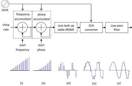
accumulators which increment their accumulated total by their respective input, once per clock cycle. The resulting phase samples address a sine look-up table (LUT) stored in a read-only memory (ROM), and the ROM outputs are converted to analog form using a digital-to-analog converter (DAC) (see
Figure 8).
Figure 8 Dual-accumulator chirp DDS architecture and signal flow. From left to right: (i) a digital frequency accumulator is initiating at a start frequency and incremented by a frequency increment, determined by the desired chirp rate, on each clock cycle, to generate a linearly increasing digital frequency; (ii) the output of the frequency accumulator is input to a second phase accumulator, which generates a quadratically increasing phase; (iii) the phase samples are used to address a look-up table, implemented as a ROM, which contains amplitudes of the sine wave for a number of phase values on the interval 𝟎, 𝟐𝝅 . The result is a chirp in the digital domain; (iv) the digital chirp is converted to analog form using a digital-to-analog converter (DAC). Due to the zero-order-hold property of the DAC, discussed in Section 2.3, the DAC output has a ‘step-like’ shape and contains higher-order harmonics of the desired output signal; (v) the DAC output is passed through a low-pass interpolating filter to remove the higher-order harmonics and obtain the desired chirped output signal. (After (Adler, Viveiros et al. 1995)).
Because DDS chirps are digitally controlled, they have excellent chirp linearity and stability. A DDS can also rapidly “hop” between frequencies, limited only by transients of its low-pass filter, and is less susceptible to thermal drift and aging. However, the quantization from a continuous
representation to a discrete one generates a deviation (or error) in the phase and amplitude which causes spurious signals to appear, degrading the linearity of the frequency sweep.
Further, due to limitations in the speed of its digital circuitry and DAC, DDS has a limited frequency range: current state-of-the-art commodity DDS ICs are clocked at 1 GHz (Analog Devices 2010), giving them usable outputs to the lower UHF spectrum, approximately 400 MHz. In order to take advantage of DDS attributes at microwave frequencies, some form of upconversion is required.
start frequency
start phase chirp
rate
sine look-up table (ROM)
D/A converter
Low-pass filter frequency
accumulator
phase accumulator clock
[image:12.595.85.525.201.487.2]13 1.3.1 Upconversion by mixing
The upconversion method we investigate in this thesis is the so-called DDS/mixer hybrid (Vankka 2000) depicted in Figure 9. The DDS chirp is generated at intermediate frequency, within the capacity of the digital components. The intermediate signal is then mixed to the desired output frequency, and alias components are filtered. If the intermediate output carrier frequency is much lower than the transmit frequency, up-mixing results in components that lie relatively close to the desired components in the frequency spectrum. The filtering of these unwanted frequencies can become a very demanding task, and several stages of mixing and filtering might be required (Cushing 2000; van Rooyen and Lourens 2000).
Figure 9 DDS/mixer hybrid. As explained in detail in Section 3.1.2, a chirp DDS at intermediate frequency (IF) is mixed with a local oscillator whose frequency is the difference between the radio frequency (RF) of the desired output and the IF. The output from the mixer is passed through a bandpass filter to select the upper sideband, so that the desired output at RF is obtained.
A distinct advantage of the DDS/mixer hybrid is the ability to generate very low phase noise output, due to the use of components (such as mixers) with negligibly low residual phase noise, compared with the base frequency source. This method also provides excellent sweep-to-sweep coherence, which is essentially limited by drifting of the X-band local oscillator.
A disadvantage of the DDS/mixer hybrid, however, is the remaining presence of the spurious signals due to the digital chirp generation. Within the digital domain, there are actually three sources of errors:
1) Sampling of the modulating signal. In so-called dual-clock architectures, the frequency accumulator is updated at a lower rate than the phase accumulator. The effect is a ‘staircase’ approximation of ideal linear time-frequency characteristic of the chirp. The ramifications of this error on the beat signal spectrum have been investigated by Salous and Green (Salous and Green 1994).
2) Phase truncation. Prior to addressing the sine ROM, the value of the phase accumulator is truncated, and only the most significant bits are used to look up the sine amplitude. This is done to reduce requirements on the memory of the ROM.
3) Amplitude quantization. As the DAC can only produce a finite number of amplitudes, the amplitude of each sample is quantized or ‘rounded’ from its ideal value.
The effect of the ‘staircase’ approximation has been investigated by Salous and Green (Salous and Green 1994). To the best of our knowledge, the effects of phase truncation and amplitude
chirp DDS
local oscillator IF
RF – IF
RF
14 quantization on the performance of FMCW radar has not been described in the extant literature. According to Stove (Stove 2004), however, the practical effects of amplitude quantization are well described by modeling it as noise which is uniformly distributed over ±0.5 bits.
1.4
This thesis
This thesis makes a contribution towards the understanding of these spurious signals by analyzing and simulating the effects of digital phase errors on the beat spectrum of a FCMW-Doppler radar employing a direct digital chirp synthesizer. Specifically, we focus on the two sources of digital phase errors, namely, the sampling of the modulating signal and phase truncation. The effects of amplitude truncation and DAC nonlinearities, the latter of which become increasingly important at higher output frequencies, are not investigated in this work.
15
2
Theory of operation of a model FMCW-Doppler transceiver
In this chapter, we review the fundamentals of homodyne FMCW-Doppler radar, and present a model system which employs a direct digital chirp synthesizer (DDCS) in its transmitter. The model system also serves as an example in subsequent chapters, where we analyze the effect of digital phase errors on its performance.
An outline of this chapter is as follows. In Section 2.1, we briefly describe the architecture and operation of the model FMCW-Doppler transceiver. In Section 2.2, we tutorially review the theory behind FMCW-Doppler signal processing, and explain how target range and velocity information can be extracted from the received echoes. In Section 2.3, we describe in more detail the operation of the DDCS, and enumerate sources of error. Finally, in Section 2.4, we formulate our research question using the fundamentals established in this chapter.
2.1
Description of the model system
In this section, we describe the architecture of our model FMCW-Doppler transceiver and briefly describe its operation. The brief description of the operation of the microwave FMCW surveillance radar given here concerns only those aspects of the FMCW radar that are needed to develop the Doppler data processing concept.
A simplified block diagram of our model FMCW Doppler radar is shown in Figure 10. At its heart is a direct digital chirp synthesizer (DDCS), clocked by a 1 GHz master clock, which generates a chirp in the digital domain and converts it to analog form using an integrated digital-to-analog converter (DAC). The output is passed through a low-pass interpolating filter to produce a chirp at
intermediate frequency (IF), which is converted up to radio frequency (RF) by a mixer and a bandpass filter6. The upconverted signal is transmitted through a transmit (TX) antenna. After reflection off a target, an echo is received by a receive (RX) antenna and fed to the RF port of a frequency mixer. Simultaneously, the local oscillator (LO) port of the mixer is fed by a ‘reference’ signal which is a version of the transmitted signal obtained through a directional coupler7. The mixing process produces a ‘beat’ signal which contains the range information obtainable from the radar.
6
Practical implementations of single-sideband (SSB) upconversion often use a pair of cascaded mixers and bandpass filters to reduce requirements on the transition width of the individual bandpass filters.
7 Typically, an image reject mixer (IRM) is used in order to reduce noise from the image sideband, which can
16
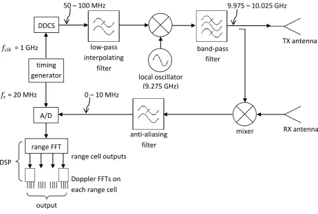
Figure 10 Simplified block diagram of a FMCW-Doppler transceiver. A direct digital chirp synthesizer (DDCS) generates a linear chirp from 50 MHz to 100 MHz, which is passed through a low-pass interpolating filter to eliminate higher harmonics. The resulting signal at intermediate frequency (IF) is mixed with a local oscillator at 9.275 GHz. The resulting double-sideband (DSB) signal is passed through a band-pass filter to select the upper sidelobe, which is a chirp from 9.975 GHz to 10.025 GHz. The main part of this chirp is transmitted through a transmit (TX) antenna while a portion is coupled to the local oscillator (LO) of a second mixer. The radio frequency (RF) port of the second mixer is fed by a separate receive (RX) antenna. The output of the second mixer is passed through an anti-aliasing filter with a cutoff frequency of 10 MHz. The resulting bandlimited signal is sampled by an analog-to-digital (A/D) converter at a rate of 𝒇𝒔 =
20 MHz, and resulting time series is fed to a digital signal processing (DSP) unit, which performs the range and Doppler fast Fourier transform (FFT) operations required to output a range-Doppler profile of the target scene.
After passing an analog anti-aliasing filter, which ensures that beat frequencies above half the sample frequency cannot pass8, the beat signal is sampled by a 16-bit analog-to-digital converter (ADC) at a rate of 𝑓𝑠 = 20 MHz using 𝑁 = 10,000 samples on each upgoing sweep of the modulating
sawtooth signal. The ADC collects 𝑁 samples in each of 𝑀 consecutive sweeps (the coherent processing interval). The samples are arranged in a 𝑀 × 𝑁 matrix, in which the rows consist of samples collected within each sweep, or in fast time, and the columns of samples collected across sweeps, or in slow time.
After weighting the rows of this matrix by a window function to reduce sidelobes (see Section 2.2.6), a first FFT is performed over the rows of the matrix. The output of the FFT is a complex array, of
8 Although not shown in the figure, the IF signal is typically also passed thorugh a high-pass filter which
compensates for the dependence of signal strength on radar distance by using a gain function that increases by 6 dB/octave. This prevents strong returns from close-in targets from saturating the receiver, and is called ‘range gain control’ (Stove 1992) or ‘sensitivity frequency control’ in analogy to ‘sensitivity time control’ used in pulse radars (Skolnik 2008).
A/D DDCS
local oscillator (9.275 GHz) 𝑓𝑐𝑙𝑘 = 1 GHz
GHZGHz
timing generator 𝑓𝑠 = 20 MHz
GHZGHz
50 – 100 MHz MHMhz.5 MHz GHZGHz
9.975 – 10.025 GHz MHMhz.5 MHz GHZGHz
range FFT
output
Doppler FFTs on each range cell range cell outputs
TX antenna RX antenna mixer anti-aliasing filter low-pass interpolating filter band-pass filter
0 – 10 MHz MHMhz.5 MHz GHZGHz
17 which only the first 𝑁/2 points are retained. The signals at each of these points then correspond to radar target echo signals that come from progressively greater ranges9. These 𝑁/2 complex array
points are collected as rows of a matrix every sweep repetition interval until a total of 𝑀 rows are obtained, over a period of time that corresponds to the reciprocal of the desired Doppler frequency resolution. Then another window vector multiples each column (or range cell) of this matrix, and a second FFT is performed over each column. The latter provides Doppler processing of each range cell, and since it operates on a complex input array, the output preserves the sense of Doppler (positive or negative), just as though in-phase and quadrature channels had been used (Barrick, Lipa et al. 1994). These digital processing steps can be implemented using field programmable gate arrays (FPGAs) or commercially available digital signal processing (DSP) boards.
In actual radar applications, the output range-Doppler data serves as input to a target tracking algorithms, which can greatly improve the detection of targets against a background of noise. Here, however, we are interested on the effects of certain hardware non-idealities on raw range-Doppler data itself. However, before discussing these effects (Section 2.3), we first explain in more detail how the range-Doppler data is obtained.
2.2
FMCW Doppler signal processing
The objective of this section is to present a simple and concise analysis – backed by an example – of the application of a FMCW signal format in radar systems. Following Barrick (Barrick 1973), it is shown how both time-delay (range) and Doppler (radial velocity) information can be extracted unambiguously.
2.2.1 Application
For the sake of illustration, we pick the following application and example. The RF radar carrier frequency is to be 𝑓𝑐 = 10 GHz10. Targets are to observed by the radar out to a range of 15 km
(corresponding to time delays up to 100 μs). At a center frequency of 10 GHz, echoes from targets moving at a velocity of up to 15 m/s in the radar’s line of sight will Doppler shifts of less than 1 kHz. In order to display such echoes unambiguously, a sweep repetition frequency (SRF) of 2 kHz is selected, corresponding to a sweep repetition interval (SRI) of 500 μs. To show sufficient detail, a Doppler processing resolution of 31.25 Hz is desired, and a range resolution of 3.75 m is desired; the latter two requirements translate, as we show in subsequent sections, to a coherent integration time of 32 ms and a chirp bandwidth of 50 MHz.
2.2.2 Transmitted signal
We select a 100% duty factor signal whose frequency sweeps upward, linearly, over one sweep repetition interval 𝑇 (𝑇 = 500 μs for our example). Since a 50 MHz bandwidth is desired, the signal can be written
𝑠𝑇𝑋 𝑡 = 𝑉𝑇𝑋cos 2𝜋 𝑓𝑐𝑡 +1
2𝛼𝑡2 ≡ 𝑉𝑇𝑋cos 𝜙𝑇𝑋 𝑡 , (1.4)
9 Actually, what is actually measured is the “pseudo-range” since Doppler frequency shifts cannot yet be
distinguished from target beat frequencies. Typically, however, the Doppler frequency shift corresponds to less than one range cell.
10 A radar operating at a center frequency of 10 GHz is said to operate in the X-band, which extends from 8.0
18 for − 𝑇 2 < 𝑡 < 𝑇 2, with repetition satisfying
𝑠𝑇𝑋 𝑡 + 𝑇 = 𝑠𝑇𝑋 𝑡 , ∀𝑡. (1.5)
Here 𝑓𝑐 denotes the center frequency (𝑓𝑐 = 10 GHz) and 𝛼 the chirp rate, which is defined as the ratio
of the chirp bandwidth 𝐵 to the sweep repetition interval 𝑇 (𝛼 = 100 GHz/s for our example). It is assumed that the signal is periodic, and hence phase-coherent from one repetition interval to the next11.
It has been found useful to define the internal time 𝑡𝑚 within the 𝑚th pulse as12
𝑡𝑚 = 𝑡 − 𝑚𝑇, −𝑇
2 < 𝑡𝑚 < 𝑇
2, (1.6)
so that (1.4) and (1.5) can be expressed as
𝑠𝑇𝑋 𝑡 = 𝑉𝑇𝑋cos 2𝜋 𝑓𝑐𝑡𝑚 +
1
2𝛼𝑡𝑚2 . (1.7)
Since the instantaneous frequency, 𝑓𝑇𝑋 𝑡 , is the derivative of the phase (Carson 1922), we have
𝑓𝑇𝑋 𝑡 = 1 2𝜋
𝑑𝜙𝑇𝑋
𝑑𝑡 = 𝑓𝑐+ 𝛼𝑡𝑚. (1.8)
where 𝑓𝑐 = 10 GHz and 𝛼 = 10 GHz/s. Thus it can be seen that the frequency excursion of 𝑓𝑇𝑋 𝑡 over
one sweep repetition interval is
Δ𝑓𝑇𝑋 = 𝐵 = 50 MHz. (1.9)
The amplitude of the transmitted signal is taken to be unity. The plot of instantaneous frequency vs. time of the transmitted signal is shown as a solid line in Figure 11.
11 FMCW radars in which the transmit phase has a fixed phase relationship from sweep to sweep, i.e.,
𝜙𝑇𝑋 𝑡 + 𝑇 − 𝜙𝑇𝑋 𝑡 = constant, are called coherent. The provision of a coherent system is prerequisite for
Doppler processing. It also allows for coherent integration over a number of sweeps, 𝑁, which improves the signal-to-noise ratio (SNR) by a factor of 𝑁, which is greater than the factor of 𝑁 typically obtainable with non-coherent integration (Beasley and Lawrence 2006).
12 In the radar signal processing literature, the internal time 𝑡
𝑚 within the 𝑚th sweep is often referred to as
19
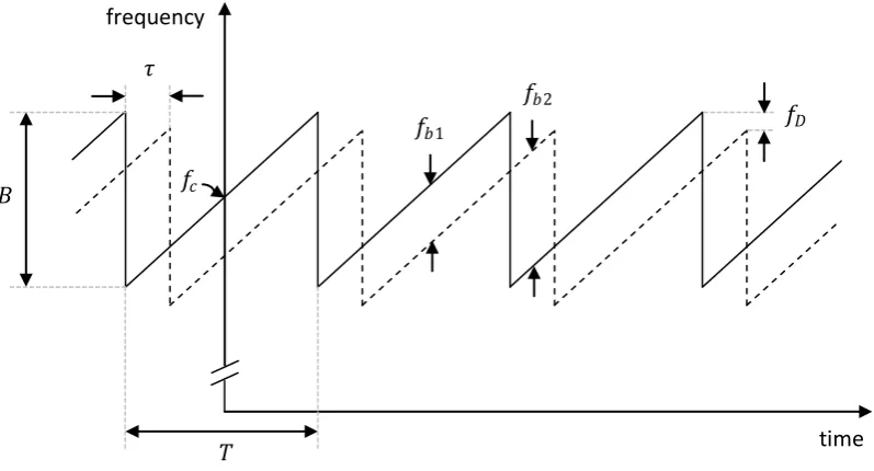
Figure 11 Frequency vs. time of transmitted and delayed/Doppler-shifted received signals. The transmitted chirp (solid line) has a carrier frequency 𝒇𝒄, peak-to-peak frequency deviation 𝑩, and sweep period 𝑻. The received signal (dashed
line) is delayed by the target round-trip delay 𝝉 and shifted by the Doppler frequency 𝒇𝑫.
2.2.3 Received signal
The received signal is both delayed in time and shifted in Doppler. To illustrate the situation, we assume that we have a discrete or ‘point’ target13 at range 10 km and travelling away from the radar at 𝑣 = 7.5 m/s. At time 𝑡 = 0, the target is exactly at 𝑅0 = 10 km from the radar. After that, its range is
a function of time as
𝑅 𝑡 = 𝑅0+ 𝑣𝑡. (1.10)
The received signal from this ‘point’ target is just a replica of the transmitted signal, but with a different amplitude 𝑉𝑅𝑋 and delayed in position by a factor 𝜏, where 𝜏 = 2𝑅 𝑡 /𝑐14. It is thus
𝑠𝑅𝑋 = 𝑉𝑅𝑋cos 2𝜋 𝑓𝑐 𝑡𝑚 − 𝜏 +1
2𝛼 𝑡𝑚 − 𝜏 2 ≡ 𝑉𝑅𝑋cos 𝜙𝑅𝑋 𝑡 (1.11)
for − 𝑇 2 + 𝜏 < 𝑡𝑚 < 𝑇 2. Its frequency is shown in Figure 11 as the dashed curve.
As seen from Figure 11, the received waveform appears to have the same sawtooth modulation of frequency as the transmit signal, but merely delayed in time and shifted in frequency. Physically, this can be explained as follows. A given transmitted waveform returns, after reflection from a ‘point’ target approaching the radar at a constant velocity, compressed in time by a certain factor (namely, 1 − 2𝑣/𝑐). Thus, a sine wave appears to be shifted in frequency by an amount proportional to the
13
The ideal ‘point’ target produces a sinusoidal beat signal. In general, however, several targets will be present within the instrumented range, and propagation along the radar path is described by a superposition of a large number of such point targets. However, because the Fourier transform is a linear operator, its response to a weighted sum of sinusoids is just the appropriately weighted sum of ‘point’ target responses. Consequently, a great deal can be learned about the radar by studying its point-target response. This approach separates algorithm and hardware effects from target and interference phenomenology (Soumekh 1999).
14 This statement actually represents an approximation which his valid in the case 𝑣 ≪ 𝑐, which of course is the
case for all targets of interest. For a derivation of this approximation, we refer the reader to Hymans and Lait (Hymans 1960) or Kelly and Wishner (Kelly and Wishner 1965).
𝑓𝑐
𝑇 frequency
𝑓𝐷
𝐵
𝑓𝑏1
𝑓𝑏2 𝜏
20 transmitted frequency. When this sine wave (carrier) is modulated, the echo returns with a higher carrier frequency and with a slightly compressed modulation. For example, an FMCW signal returns with a higher sweep repetition frequency and a higher chirp rate than it had when it left the transmitter. The effects on the modulation are often small, however, and can often be neglected. A criterion for the validity of this approximation can easily be obtained and expressed in terms of the time-bandwidth product of the transmitted modulation. Since a single sweep has a duration 𝑇, its echo has a duration 𝑇 1 − 2𝑣/𝑐 ≡ 𝑇 − Δ𝑇. This change in length will be noticeable only if Δ𝑇 is comparable to the inverse of the bandwidth 𝐵 of the signal, which measures the “complexity” of the signal and the range accuracy obtainable. Thus, the Doppler stretch effect on the modulation signal can be ignored only if Δ𝑇 ≪ 1/𝐵, which is equivalent to (Kelly and Wishner 1965)
2𝑣
𝑐𝐵𝑇 ≪ 1. (1.12)
In the present example, the maximum value of 2𝑣/𝑐 is 1 × 10⁻⁷, whereas the time-bandwidth product 𝐵𝑇 is 25,000 so 2 𝑣/𝑐 𝐵𝑇 = 0.0025 and this approximation is justified. As a result, the received echo can be considered modulated in the same way as the transmitted signal, but shifted in frequency by the Doppler frequency
𝑓𝐷 ≡2𝑣
𝑐 𝑓𝑐. (1.13)
For a target receding at 7.5 m/s in the radars line of sight and a center frequency of 10 GHz, the Doppler frequency is 500 Hz.
2.2.4 Beat signal
Now after RF amplification, the received signal is ‘dechirped’ or ‘deramped’ by ‘mixing’ or ‘beating’ it together with a replica of the transmitted signal in a frequency mixer15. The resulting signal will contain a product term 𝐺𝑉𝑇𝑋𝑉𝑅𝑋cos 𝜙𝑇𝑋cos 𝜙𝑅𝑋, where 𝐺 is a numerical constant accounting for
the voltage conversion loss of the mixer, and other higher-order products. In general, only the lowest-order product will have significant amplitude. The product may be expanded as a sum, namely
1
2𝐺𝑉𝑇𝑋𝑉𝑅𝑋 cos 𝜙𝑇𝑋 − 𝜙𝑅𝑋 + cos 𝜙𝑇𝑋 + 𝜙𝑅𝑋 .
The phase-sum term is an oscillation at twice the carrier frequency, which is generally filtered out either actively, or more usually in radar systems because it is beyond the cut-off frequency of the mixer and subsequent receiver components (Brooker 2005). We are thus interested in the function
1
2𝐺𝑉𝑇𝑋𝑉𝑅𝑋cos 𝜙𝑇𝑋− 𝜙𝑅𝑋 , which is called the beat signal:
𝑠𝑏 =1
2𝐺𝑉𝑇𝑋𝑉𝑅𝑋cos 𝜙𝑇𝑋− 𝜙𝑅𝑋 ≡ 𝑉𝑏cos 𝜙𝑏. (1.14)
15
A mixer is a three-port device that uses a nonlinear or time-varying element to achieve frequency conversion. In its down-conversion configuration, it has two inputs, the radio frequency (RF) signal and the
21 Thus, the mixing of the received signal with a replica of the transmitted signal is represented
mathematically by subtracting the phase 𝜙𝑅𝑋 from 𝜙𝑇𝑋.
By taking the time derivative of this relation, it follows that the instantaneous frequency of the beat signal, 𝑓𝑏 𝑡 , is equal to
𝑓𝑏 𝑡 = 𝑓𝑇𝑋 𝑡 − 𝑓𝑅𝑋 𝑡 , (1.15)
where 𝑓𝑅𝑋 𝑡 ≡ 𝑓𝑇𝑋 𝑡 − 𝜏 is the instantaneous frequency of the received signal. The mixture of the
[image:21.595.70.490.256.569.2]transmitted and received sawtooth frequency waveforms and their subtraction, as shown in Figure 11, thus produces a beat signal whose instantaneous frequency is shown in Figure 12(a).
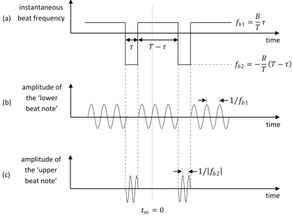
Figure 12 Frequency and amplitude plots versus time of the beat signal. In (a), we see that the instantaneous frequency of the beat signal, 𝒇𝒃 𝒕 , alternates between two distinct tones, 𝒇𝒃𝟏 and 𝒇𝒃𝟐. As a result, the beat signal 𝒔𝒃 can be
regarded as the sum of two pulse trains; (b) illustrates the ‘lower beat note’ at 𝒇𝒃𝟏, and (c) the ‘upper beat note’ at 𝒇𝒃𝟐.
As seen from Figure 12(a), the beat frequency alternates between two distinct tones. In the 𝑚th interval, these two frequencies are16
(i) During time − 𝑇 2 < 𝑡𝑚 < − 𝑇 2 + 𝜏,
when 𝑓𝑅𝑋 = 𝑓𝑐 +𝐵𝑇 𝑡𝑚 −1− 𝜏
16 Here, we implicitly assume that 𝜏 < 𝑇, or equivalently, 𝑅 < 𝑐𝑇/2. The range 𝑐𝑇/2 is called the radar’s
unambiguous range; typically, the instrumented range 𝑅𝑚𝑎𝑥 is chosen at less than 20% of the unambiguous range so that the overlap loss is less than 1.9 dB.
𝜏 time
𝑓𝑏2= −𝐵
𝑇 𝑇 − 𝜏 𝑇 − 𝜏
𝑓𝑏1 =𝐵 𝑇𝜏 (a)
1/𝑓
𝑏11/ 𝑓
𝑏2(b)
(c)
amplitude of the ‘upper beat note’ amplitude of
the ‘lower beat note’ instantaneous beat frequency
𝑡𝑚 = 0
time
22 and 𝑓𝑇𝑋 = 𝑓𝑐 +𝐵𝑇𝑡𝑚,
𝑓𝑏 𝑡 = −𝐵
𝑇 𝑇 − 𝜏 ≡ 𝑓𝑏2, (1.16)
(ii) During time − 𝑇 2 + 𝜏 < 𝑡𝑚 < 𝑇 2,
when 𝑓𝑅𝑋 = 𝑓𝑐 +𝐵𝑇 𝑡𝑚 − 𝜏
and 𝑓𝑇𝑋 is as in (i),
𝑓𝑏 𝑡 =𝐵
𝑇𝜏 ≡ 𝑓𝑏1. (1.17)
The beat signal can thus be represented as the sum of two pulse trains as shown in Figure 12(b) and Figure 12(c). One, the ‘lower beat note’, is at frequency 𝑓𝑏1 and the width of its pulses is 𝑇 − 𝜏. The
other, the ‘upper beat note’, is at frequency 𝑓𝑏2 and the width of its pulses is 𝜏.
The ‘upper beat note’ 𝑓𝑏2 occurring during − 𝑇 2 < 𝑡𝑚 < − 𝑇 2 + 𝜏 is offset in frequency from the
‘lower beat note’ 𝑓𝑏1 by the sweep width, 𝐵, as shown by equations (1.16) and (1.17). This is
because during − 𝑇 2 < 𝑡𝑚 < − 𝑇 2 + 𝜏, the local oscillator starts the 𝑚th sweep while the
received RF signal corresponds to the 𝑚 − 1 th sweep. Since 𝐵 is much greater than the
bandwidth of the receiver, the mixer output for − 𝑇 2 < 𝑡𝑚 < − 𝑇 2 + 𝜏 will therefore be filtered
and rejected. Hence, for − 𝑇 2 < 𝑡𝑚 < − 𝑇 2 + 𝜏 the beat signal will be a transient pulse. If an ADC
is used to observe the beat signal, the sampling can be delayed at the start of each sweep so that the ‘fly-back’ or ‘retrace’ effects of the local oscillator returning to its starting frequency are omitted. Therefore, we are left with a single pulse train to analyze: the ‘lower beat note’. Inserting (1.7) and (1.11) into (1.14), we obtain
𝑠𝑏 𝑡 = 𝑉𝑏cos 2𝜋 𝑓𝑐𝑡𝑚 +1
2𝛼𝑡𝑚2 − 2𝜋 𝑓𝑐 𝑡𝑚 − 𝜏 + 1
2𝛼 𝑡𝑚 − 𝜏 , −
𝑇
2+ 𝜏 < 𝑡𝑚 < 𝑇 2
or, simplifying,
𝑠𝑏 𝑡 = 𝑉𝑏cos 2𝜋 𝑓𝑐𝜏 + 𝛼𝜏𝑡𝑚 −1
2𝛼𝜏2 , − 𝑇
2+ 𝜏 < 𝑡𝑚 < 𝑇
2. (1.18)
The two-way propagation delay 𝜏 is also time-dependent, and is referenced to the range at 𝑡 = 0 so that
𝜏 𝑡 =2𝑅 𝑡
𝑐 =
2
𝑐 𝑅0+ 𝑣𝑡 = 2
𝑐 𝑅0+ 𝑣 𝑡𝑚 + 𝑚𝑇 ≡ 𝜏0+ 𝛽𝑡𝑚 + 𝛽𝑚𝑇, (1.19)
where 𝜏0≡ 2𝑅0/𝑐 is the transit time corresponding to the initial range and 𝛽 ≡ 2𝑣/𝑐 is the
normalized velocity. The term 𝛽𝑚𝑇 is the increase in transition time due to the accumulated range 𝑣𝑚𝑇 from 𝑡 = 0 to the middle of the 𝑚th sweep. This term provides the only difference for the equations for consecutive sweeps as opposed to a single sweep.
With equations (1.18) and (1.19) and some algebra, it follows that
23 for − 𝑇 2 + 𝜏 < 𝑡𝑚 < 𝑇 2, where
𝐶1= 𝑓𝑐𝜏0−1
2𝛼𝜏02+ 𝑓𝑐𝛽𝑚𝑇 − 𝛼𝜏0𝛽𝑚𝑇, (1.21)
𝐶2= 𝑓𝑐𝛽 + 𝛼𝜏0+ 𝛼𝛽𝑚𝑇 − 𝛼𝜏0𝛽 − 𝛼𝛽2𝑚𝑇, (1.22)
and
𝐶3 = 𝛼𝛽 1 −
𝛽
2 . (1.23)
Hence, we have three contributions to the phase: a constant, a linear term in 𝑡𝑚, and a quadratic
term in time, 𝑡𝑚2. Equations (1.20) through (1.23) can be simplified by discarding all terms for which
the phase contribution is negligible. The maximum phase contribution for the time-dependent terms occurs when 𝑡𝑚 = 𝑇/2. Each term must be examined to determine if it is small compared to 𝜋
radians.
With the parameters of Table 2 and assuming that the number of sweeps to be processed is of the order of 𝑚 ≅ 100, the fourth term in (1.21), 𝛼𝜏0𝛽𝑚𝑇, is of the order of 0.16 radian and can be
discarded. Similarly, the linear terms 𝛼𝜏0𝛽 and 𝛼𝛽2𝑚𝑇 in (1.22) contribute at most 0.0016 and 8 ×
10-9 radians to the phase, respectively. Finally, the quadratic term in (1.20) is always small within the interval − 𝑇 2 + 𝜏 < 𝑡𝑚 < 𝑇/2; for example, at 𝑡𝑚 = 𝑇/2, it is of the order of 0.0003 radian.
Equation (1.20) then simplifies to
𝑠𝑏,𝑚 𝑡𝑚 = 𝑉𝑏cos 2𝜋𝑓𝑏,𝑚𝑡𝑚+ 𝜙𝑚 , −𝑇
2+ 𝜏 < 𝑡𝑚 < 𝑇
2, (1.24)
where the frequency of the beat signal is
𝑓𝑏,𝑚 = 𝑓𝑐𝛽 + 𝛼𝜏0+ 𝛼𝛽𝑚𝑇 (1.25)
and the phase is
𝜙𝑚 = 2𝜋 𝑓𝑐𝜏0− 𝛼𝜏02 + 𝑓2
𝑐𝛽𝑚𝑇 ≡ 𝜙0+ 2𝜋𝑓𝐷𝑚𝑇. (1.26)
The three terms that comprise the frequency term are
(a) The usual range term for a FMCW radar, 𝛼𝜏0 or 2𝐵/𝑐𝑇 𝑅0;
(b) The Doppler shift 𝑓𝐷, since 𝑓𝑐𝛽 = 2𝑣 𝜆𝑐 = 𝑓𝐷; and
(c) A term resulting from the accumulated range. The accumulated range is 𝑣𝑚𝑇, and since the frequency dependence on range is 2𝐵/𝑐𝑇 𝑅, the accumulated range causes an increase in beat frequency 2𝐵 𝑐𝑇 𝑣𝑚𝑇 = 𝛼𝛽𝑚𝑇 = 𝛽𝑚𝐵.
The two terms that comprise the phase of the signal are:
(a) 𝑓𝑐𝜏0, the total number of cycles of 𝑓𝑐 that occur during the round-trip propagation time
corresponding to the initial range;
(b) −𝛼𝜏02/2, a range-dependent phase term which is incidentally called the “residual video
24 (c) 𝑓𝑐𝛽𝑚𝑇, the number of cycles of 𝑓𝑐 that occur during time 𝛽𝑚𝑇, the round-trip propagation
time for the accumulated range.
Both the frequency, 𝑓𝑏,𝑚, and the phase, 𝜙𝑚, of the beat signal change from sweep to sweep. The
frequency change is caused by the range change during the sweep time. With the parameters assumed above, the total observation time (𝑀𝑇) is 50 ms, and with a velocity of 7.5 m/s, the change in range is only 0.375 m. This is much less than the range resolution assumed (3.75 m). Hence the frequency change during the 𝑀 sweeps is small compared to the range term, except for the very shortest ranges, and the term 𝛼𝛽𝑚𝑇 in (1.25) is also negligible. The radian phase change from sweep to sweep is 2𝜋𝑓𝐷𝑇, or about 0.067𝜋 radians m/s of velocity. Note that a velocity of ±𝜆𝑐/4𝑇
or 15 m/s will cause a phase shift of 𝜋 radians between consecutive sweeps. When the phase shift is this large it is not possible to determine if the phase in increasing from sweep to sweep (positive velocity) or decreasing (negative velocity).
Two other effects occur within the pulse; its width, being 𝑇 − 𝜏, changes very slightly from pulse to pulse. Since 𝑇 = 500 μs, 𝜏 = 𝜏0+ 𝛽𝑚𝑇 we have for 𝑚 = 0, 𝑇 − 𝜏 = 400 μs; for 𝑚 = 100 we have
𝑇 − 𝜏 = 400 μs – 2.5 ns. Thus the change in pulse width is negligible. A very important second effect, however, is the change in phase from pulse to pulse, as represented by the third term in (1.26). This phase change shall in fact prove to be the basis for the Doppler processing.
2.2.5 Double-FFT digital processing
Here we demonstrate how a double Fourier-transformation process can be used – often in real time using the fast-Fourier-transform (FFT) algorithm – to produce a time-delay (range) and Doppler (velocity) display of the radar target data. The first Fourier transform process is performed over a pulse repetition period, 𝑇 (i.e., within a pulse) to obtain target range. The second Fourier transform is performed over several pulses of these data to obtain target Doppler velocity.
2.2.5.1 Range FFT
First, let us perform a Fourier transform on a single pulse. This is shown in Figure 13. In order to perform the Fourier transform digitally, the beat signal is sampled in by an analog-to-digital converter (ADC), after which a fast Fourier transform (FFT) is performed on the resulting samples. We discuss two practical aspects relating to the A/D conversion.
Sampling interval. In order to avoid sampling ‘fly-back’ transients from the previous sweep, the beat signal is sampled on an interval
𝑇𝐴𝐷 ≡ 𝑇 − 𝜏𝑚𝑎𝑥 (1.27)
so that the ‘lower’ beat signal is observed for all targets within the instrumented range, and the ‘upper’ beat signal is omitted (cf. (Wojtkiewicz, Misiurewicz et al. 1997)). For the parameters of our example, the sampling interval is 𝑇𝐴𝐷 = 500 μs – 100 μs = 400 μs.
Sampling rate criterion. In order to satisfy the Nyquist sampling criterion, we have to sample at a rate 𝑓𝑠 that is at least twice the maximum value the beat frequency 𝑓𝑏 can assume:
𝑓𝑠 ≥ 2𝑓𝑏,𝑚𝑎𝑥. (1.28)
Since for our example the maximum beat frequency is 𝑓𝑏,𝑚𝑎𝑥 = 10 MHz, a sampling rate of 𝑓𝑠
25
𝑁 ≡ 𝑓𝑠𝑇𝐴𝐷, (1.29)
or 𝑁 = 10,000 for the example considered here17.
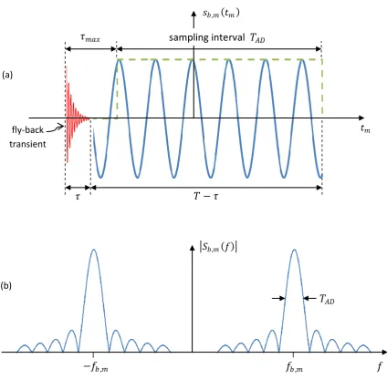
[image:25.595.73.498.171.587.2]In Figure 13(a), we depict a fly-back transient, and illustrate the concept of sampling on a ‘fly-back free interval’.
Figure 13 Single pulse and its Fourier transform. (a) Illustrates a single pulse of the ‘lower’ beat signal 𝒔𝒃,𝒎 𝒕𝒎 during
one sweep repetition interval. During the initial transit time 𝝉 following the beginning of each sweep, the beat signal is a transient pulse due to the ‘fly-back’ of the local oscillator to its starting frequency and the filtering of the ‘upper’ beat note. In order to avoid sampling this ‘retrace’ effect, the sampling is delayed from the beginning of the sweep by the maximum transit time 𝝉𝒎𝒂𝒙 (cf. (Piper 1995). (b) The amplitude spectrum 𝑺𝒃,𝒎 𝒇 of 𝒔𝒃,𝒎 𝒕𝒎 consists of two “sicn”
pulses centered at −𝒇𝒃,𝒎 and 𝒇𝒃,𝒎. (After (Barrick 1973)).
The Fourier transform of beat signal in the 𝑚th pulse, 𝑠𝑏,𝑚 𝑡𝑚 as given by (1.24), is
17
In order to avoid out-of-band noise from folding back into the target beat signal spectrum, a practical application includes an anti-alias filter with a cutoff frequency between 𝑓𝑏,𝑚𝑎𝑥 and 𝑓𝑠/2.
𝑡𝑚 𝑠𝑏,𝑚 𝑡𝑚
𝑇 − 𝜏
𝜏
sampling interval
𝑇
𝐴𝐷𝑇
𝐴𝐷𝑓
𝑓
𝑏 ,𝑚−𝑓
𝑏 ,𝑚 (b)(a)
𝜏
𝑚𝑎𝑥𝑆𝑏,𝑚 𝑓
26 𝑆𝑏,𝑚 𝑓 = 𝑇 2 𝑉𝑏cos 2𝜋𝑓𝑏,𝑚𝑡 + 𝜙𝑚 𝑒−𝑗2𝜋𝑓𝑡
−𝑇 2 +𝜏𝑚𝑎𝑥
𝑑𝑡 (1.30)
or
𝑆𝑏,𝑚 𝑓 =𝑉𝑏𝑇𝐴𝐷
2 sinc 𝑓 − 𝑓𝑏,𝑚 𝑇𝐴𝐷 𝑒𝑗 𝜙0+𝑗2𝜋 𝑓𝐷𝑚𝑇 + sinc 𝑓 + 𝑓𝑏,𝑚 𝑇𝐴𝐷 𝑒−𝑗 𝜙0−𝑗2𝜋 𝑓𝐷𝑚𝑇 ,
(1.31)
where sinc ∙ is the normalized sinc function defined as
sinc 𝑥 ≡sin 𝜋𝑥
𝜋𝑥 . (1.32)
This Fourier transform is shown in Figure 13(b). Since we started with 𝑁 ≥ 2𝑓𝑏,𝑚𝑎𝑥𝑇𝐴𝐷 samples, we
obtain samples in the frequency domain from −𝑓𝑏,𝑚𝑎𝑥 to 𝑓𝑏,𝑚𝑎𝑥, i.e., at 𝑁/2 = 𝑓𝑏,𝑚𝑎𝑥𝑇𝐴𝐷 positive
values of frequency. These samples are complex in general, as evidenced by the exponential phase factor containing 𝜙0 and 2𝜋𝑓𝐷𝑚𝑇. Thus we conceptually have 𝑁/2 range bins (𝑁 2 = 5,000 here),
permitting us to realize the 3.75 m range resolution over the 15 km window, as initially stipulated. Note that each 𝑁/2 resolution element can be considered a range bin as long as the Doppler term, 2𝑣 𝑐 𝑓𝑐, is small compared to the range term, 𝛼𝜏0; this is true for the example considered here.
Since each pulse is approximately 1/𝑇𝐴𝐷 wide at the half-power point (𝑇𝐴𝐷 = 400 μs here), we should
be able to resolve 4,000 targets within range because the width of each FFT pulse in this 10 MHz window is 2.5 kHz. Hence after one FFT process within a pulse we have range information, but no Doppler information; we now turn to extraction of Doppler.
Note that is we start with the first pulse at 𝑚 = 0 and do this FFT process on each pulse, we obtain a Fourier transform 𝑚 times, where 𝑚 ≤ 𝑀 − 1 (some maximum value). Since the frequency, 𝐹𝑚, and
phase, 2𝜋𝑓𝐷𝑚𝑇, shifts slightly from pulse to pulse due to the target velocity (as given by equations
(1.25) and (1.26)), this “sinc” pulse in the frequency domain will change very slightly after each Fourier transformation. Since the 𝑁-point FFT produces numbers at 𝑁/2 discrete positive frequencies, (1.31) should really be written with 𝑓 replaced by 𝑓 =𝑘𝑁𝑓𝑠, where 𝑘 = 0, … ,𝑁2− 1.
Thus the first FFT process on 𝑁 samples within a pulse gives 𝑁/2 range bins for each pulse. For each successive pulse, this FFT gives 𝑁/2 additional positive frequency samples. Digitally, we store each 𝑁/2 samples in rows of a matrix, until we have 𝑀 rows. Thus, we have an 𝑀-by-𝑁/2 matrix whose columns so far represent range bins.
2.2.5.2 Doppler FFT
Now, we perform another FFT over each column, or range bin. This requires 𝑀 points altogether. Each matrix element is a complex number whose value changes in a column because the frequency, 𝑓𝑏,𝑚, and the phase, 2𝜋𝑓𝐷𝑚𝑇, are changing from sweep to sweep. Since each of the 𝑀 vertical
elements comes from a different pulse 𝑇 seconds apart, 𝑀𝑇 seconds are required to fill this matrix. Hence each column is really a function of time, and the 𝑀 column elements can be considered (digital) samples of this time function.
27 this produces 𝑓𝑏,𝑚 = 5 MHz + 500 Hz + 2.5𝑚 Hz. Thus for 𝑚 running from 1 to 100 – corresponding to
time running from 0 to 50 milliseconds – two things happen happen to the positive pulse in the 𝑛th range bin: its amplitude changes slightly due to the shift of the “sinc” pulse because of 𝑓𝑏,𝑚, and its
phase changes. The amplitude variation from 𝑚 = 1 to 𝑚 = 100 is slow. For the example given, the shift in the pulse due to 𝑓𝑏,𝑚 is 250 Hz over 𝑀 = 100 pulses; the -3.9 dB width of the “sinc” pulse is
1/𝑇𝐴𝐷 = 2.5 kHz. Hence amplitude variation within a column is slight, and can be represented in
most cases by a constant, i.e., sinc 𝑓 − 𝑓𝑏,𝑀/2 𝑇𝐴𝐷 , its value midway down the column where
𝑚 = 𝑀/2.
Thus the only variation now within the column (at the positive frequency corresponding to 𝑛) is the phase factor, i.e.,
𝑆𝑚𝑛 = 𝐾 𝑓 𝑒𝑗2𝜋𝑓𝐷𝑚𝑇 = 𝐾 𝑓 𝑒𝑗2𝜋 𝑓𝐷𝓉𝑚, (1.33)
where
𝐾 𝑓 =𝑉𝑏𝑇𝐴𝐷
2 sinc 𝑓 − 𝑓𝑏,𝑀/2 𝑇𝐴𝐷 𝑒𝑗 𝜙0. (1.34)
In the rightmost expression of (1.33), 𝑚𝑇 has been replaced by 𝓉𝑚 to represent the discrete flow of
time from pulse to pulse. The Fourier transform of this quantity over 𝓉𝑚 from 0 to 𝑀𝑇 is
𝒮𝑛= 𝐾 𝑓 𝑀𝑇sinc 𝑓 − 𝑓𝐷 𝑀𝑇 . (1.35)
Here again we should note that our digital FFT does not really give a continuous variation over 𝑓 (frequency), but will compute values at 𝑀 discrete frequency points. The question arises how we should choose these 𝑀 frequency points, i.e., how wide a frequency window we want to display. Since our sweep repetition frequency, 1/𝑇 (1/𝑇 = 2.5 kHz here) results in an unambiguous Doppler of 1.25 kHz, we would logically select 𝑓𝐷,𝑚𝑎𝑥 = 1/2𝑇 so as to display all of the unambiguous Doppler
window. Then the frequency window in Doppler will be from −𝑓𝐷,𝑚𝑎𝑥 to 𝑓𝐷,𝑚𝑎𝑥 at a spacing
𝑓𝐷,𝑚𝑎𝑥/𝑀, which turns out to every 2𝑓𝐷,𝑚𝑎𝑥/𝑀 Hz, or 20 Hz here. Note also in (1.33) that if the
Doppler shift 𝑓𝐷 exceeds 1/2𝑇, then from pulse to pulse we will be sampling at less than the
required Nyquist sampling rate. Hence our sweep repetition frequency, 1/𝑇, must always be at least twice the maximum expected Doppler frequency18.
Observe now an important fact in (1.35): the displacement of the “sinc” pulse resulting from the second Fourier transformation over the columns occurs at the Doppler shift 𝑓𝐷 = 2𝑣 𝑐 𝑓𝑐 that
results from a target at (radial) velocity 𝑣 with a backscatter radar having a carrier frequency 𝑓𝑐.
Furthermore, the -3.9 dB width of the pulse represented by (1.35) is 1/𝑀𝑇 Hz, as shown in Figure 14. Thus, we produce 𝑀 (or 100) Doppler frequency points every 1/𝑀𝑇 Hz (or 20 Hz here). Since 𝑀𝑇 is the coherent integration time (in this scheme, it is the time required to fill the matrix), 1/𝑀𝑇 is exactly the Doppler resolution one would expect from any coherent pulse-Doppler radar.
18 The unambiguous velocity measurement range can be extended by using multiple (appropriately chosen)
28
Figure 14 Doppler spectrum after second Fourier transformation within a given range. (After (Barrick 1973)).
Therefore, in summary, we have done two sets of FFTs. One set within each pulse at 𝑁 points to give 𝑁/2 range bins; these bins are elements of a row of a matrix. The second set is over 𝑀 pulses, or over 𝑀 column elements of the matrix, to give 𝑀 Doppler bins for each range bin. Note that the original target range also contained a small offset due to Doppler. If this offset is objectionable, it can now be removed – in the case of a discrete target – by using the Doppler information to correct the target range.
2.2.6 Sidelobe apodization
The spectrum of a truncated sine wave output by a FMCW radar for a single target has the
characteristic ‘sin x/x’ shape as predicted by Fourier theory. The range side lobes in this case are only 13.3 dB lower than the main lobe, which is not satisfactory as it can result in the occlusion of small nearby targets as well as introducing clutter from the adjacent lobes into the main lobes. To counter these undesirable effects, a window function is usually applied to the sampled IF signal prior to FFT frequency estimation.
Many window functions with a wide range of properties have been published by various authors and their effects on fixed-frequency signals well documented (e.g. see an extensive review given by Harris (Harris 1978)). Consideration in this report is restricted to three commonly employed window functions: Hamming, Hanning, and Blackman (Pace 2004). Each of these windows has the generic form
𝑤 𝑛 = 𝑎0− 𝑎1cos 2𝜋 𝑛
𝑁 − 1 + 𝑎2cos 4𝜋 𝑛
𝑁 − 1 , 0 ≤ 𝑛 ≤ 𝑁 − 1, (1.36)
where 𝑛 is the sample index, 𝑁 is the total number of samples, and 𝑎0, 𝑎1, and 𝑎2 are coefficients
specific to each window. As summarized in Table 1, the resulting spectra offer poorer resolution but improved sidelobe levels that can accommodate almost any requirement.
1/𝑀𝑇
𝒮
𝑛29
Window Rectangle Hamming Hanning Blackman
Worst side lobe (dB) –13.3 –42.2 –31.5 –58
3 dB bandwidth (bins) 0.88 1.32 1.48 1.68
Scalloping loss (dB)19 3.92 1.78 1.36 1.1
SNR loss (dB) 0 1.34 1.76 2.37
Main lobe width (bins) 2 4 4 6
𝑎0 1 0.54 0.50 0.42
𝑎1 0.46 0.50 0.50
𝑎2 0.08
[image:29.595.90.381.383.618.2]Table 1 Properties of some weighting functions. (After (Pace 2004)).
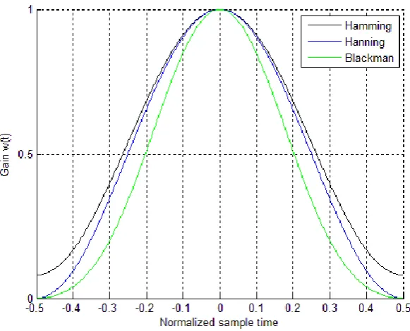
Figure 15 and Figure 16 below compare these windows in the time and frequency domains. Of particular interest are the Hamming and Hanning weighting functions that offer similar SNR and resolutions, but with completely different sidelobe characteristics. As can be seen in Figure 15, the former has the form of a squared-plus-pedestal, while the latter is just a standard cosine-squared function. In the Hamming case, the close-in side lobe is suppressed to produce a maximum level of -42.2 dB, but the energy is spread into the remaining sidelobes resulting in a falloff of only 6 dB/octave, while in the Hanning case the first lobe is higher at -31.5 dB, but with a falloff of 18 dB/octave (Willis and Griffiths 2007).
Figure 15 Window function gains. (After (Willis and Griffiths 2007)).
19
Scalloping loss is the apparent attenuation of the measured value for a frequency component that falls exactly half way between FFT bins. It is defined as the ratio of the power gain for a signal frequency component located half way between bins to that of a component located exactly on the FFT bin (source:
30
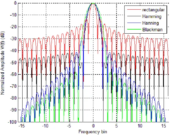
Figure 16 Normalized window amplitude spectra as a function of bin number. (After (Willis and Griffiths 2007)).
For most FMCW applications, the Hamming window is used as it provides a good balance between sidelobe levels (-42.2 dB), beam width (1.32 bins), and loss in SNR compared to a matched filter (1.34 dB) (Willis and Griffiths 2007).
2.2.7 Simulation
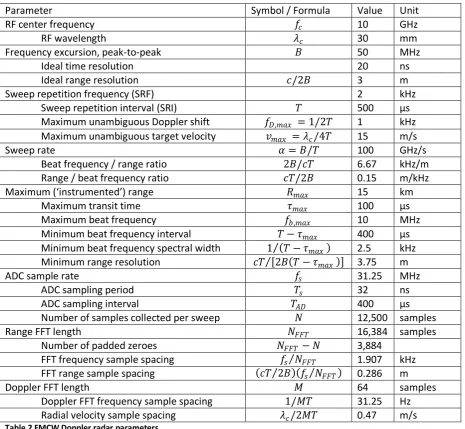
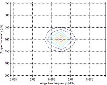
We have implemented a simulation of a FMCW Doppler radar in MATLAB. The simulation code is given in the Appendix20. The parameters of our model FMCW Doppler radar are tabulated in Table 2.
20 Actually, the code given in the Appendix also provides the ability to investigate the effect of sinusoidal phase
31
Parameter Symbol / Formula Value Unit
RF center frequency 𝑓𝑐 10 GHz
RF wavelength 𝜆𝑐 30 mm
Frequency excursion, peak-to-peak 𝐵 50 MHz
Ideal time resolution 20 ns
Ideal range resolution 𝑐/2𝐵 3 m
Sweep repetition frequency (SRF) 2 kHz
Sweep repetition interval (SRI) 𝑇 500 μs
Maximum unambiguous Doppler shift 𝑓𝐷,𝑚𝑎𝑥 = 1/2𝑇 1 kHz
Maximum unambiguous target velocity 𝑣𝑚𝑎𝑥 = 𝜆𝑐/4𝑇 15 m/s
Sweep rate 𝛼 = 𝐵/𝑇 100 GHz/s
Beat frequency / range ratio 2𝐵/𝑐𝑇 6.67 kHz/m Range / beat frequency ratio 𝑐𝑇/2𝐵 0.15 m/kHz
Maximum (‘instrumented’) range 𝑅𝑚𝑎𝑥 15 km
Maximum transit time 𝜏𝑚𝑎𝑥 100 μs
Maximum beat frequency 𝑓𝑏,𝑚𝑎𝑥 10 MHz
Minimum beat frequency interval 𝑇 − 𝜏𝑚𝑎𝑥 400 μs
Minimum beat frequency spectral width 1 𝑇 − 𝜏𝑚𝑎𝑥 2.5 kHz
Minimum range resolution 𝑐𝑇 2𝐵 𝑇 − 𝜏𝑚𝑎𝑥 3.75 m
ADC sample rate 𝑓𝑠 31.25 MHz
ADC sampling period 𝑇𝑠 32 ns
ADC sampling interval 𝑇𝐴𝐷 400 μs
Number of samples collected per sweep 𝑁 12,500 samples
Range FFT length 𝑁𝐹𝐹𝑇 16,384 samples
Number of padded zeroes 𝑁𝐹𝐹𝑇 − 𝑁 3,884
FFT frequency sample spacing 𝑓𝑠 𝑁𝐹𝐹𝑇 1.907 kHz
FFT range sample spacing 𝑐𝑇 2𝐵 𝑓𝑠 𝑁𝐹𝐹𝑇 0.286 m
Doppler FFT length 𝑀 64 samples
[image:31.595.67.533.69.498.2]Doppler FFT frequency sample spacing 1/𝑀𝑇 31.25 Hz Radial velocity sample spacing 𝜆𝑐/2𝑀𝑇 0.47 m/s Table 2 FMCW Doppler radar parameters.
In Figure 17, we show a contour plot (linear scale) of the simulated response of a ‘point’ target at an initial range 𝑅0 = 10 km receding in the radar’s line of sight direction at a velocity of 𝑣 = 7.5 m/s. We
32
Figure 17 Contour plot (linear scale) of the response of a ‘point’ target at an initial range of 10 km, receding at a radial velocity of 7.5 m/s, for the simulation parameters given in Table 2.
Figure 17 shows that the ‘point’ target response is a peak at a range beat frequency of 6.667 MHz and a Doppler frequency of 500 Hz, as expected.
2.2.8 Discussion of the ‘point’ target model
The true physics of scattering of a radar signal by a target would indicate that the ‘point’ model is too simplistic. In fact many assumptions must be made in order to end up with the above system model. For instance:
Scattering by a target can also impart a phase shift to the reflected wave, which we have omitted here. In a more general development, we would adopt a complex representation of the transmitted and received signals (Jakowatz, Wahl et al. 1996) and allow 𝑔 to take complex values to incorporate this phase shift. The phase shift can also vary with frequency, which gives rise to target ‘signature’ responses (Soumekh 1999).
The medium through which the radar signal travels is assumed to be non-dispersive. This also precludes waveguide dispersion or group delay in the filters. In practice, group delay in the filters is a significant problem (Perez-Martinez, Burgos-Garcia et al. 2001).
33 One should associate an amplitude factor with the target return, which varies with range as
~1/𝑅4 for point targets and ~1/𝑅2 for extended targets or ‘clutter’. For targets within a
range of typically 1 km, however, this amplitude factor is compensated for by a sensitivity frequency control (SFC) filter; beyond this range, the effect of this factor is often negligible compared to radar system errors such as the quantization noise, thermal additive noise, and multiplicative noise (instability of the radar) (Soumekh 1999).
Despite its limitations, however, the ‘point’ target model is a convenient way to separate algorithm and hardware effects from target and interference phenomenology.
2.2.9 Concluding remarks and outlook
We have discussed how a FMCW-Doppler transceiver transmitting coherent frequency sweeps can extract target range and velocity information. Up till now we have assumed that the transmitted chirps were ideally linear. However, a chirp generated by a direct digital chirp synthesizer (DDCS) is affected certain inherent idealities due to the digital nature of the DDCS, and these non-idealities will in turn affect the observed range-Doppler output. Before determining these effects, which is the subject of Chapters 3 and 4, we first discuss the operation of the DDCS in more detail in Section 2.3.
2.3
Direct digital synthesis
Before digital technology became widely available, analog techniques were employed to generate radar transmit waveforms. FMCW signals were generated using a voltage-controlled oscillator (VCO) or YIG (Yttrium Iron Garnet)-tuned oscillator. However, it is difficult to achieve adequate linearity over a wide bandwidth and preserve coherence from sweep to sweep, and such oscillators can be susceptible to mismatches and to drift with temperature. Digital technology, however, presents the radar system designer flexibility and accuracy of digital waveform control.
In this section, we describe the direct digital synthesis (DDS) technique commonly used to generate radar transmit signals digitally. An outline of this section is as follows. First, we