arXiv:hep-th/9909218v2 31 Mar 2000
DAMTP-1999-104 SNUTP-99-042 KIAS-P99089 hep-th/9909218
Nahm Data and the Mass of 1/4-BPS States
Conor J. Houghton,
∗DAMTP, University of Cambridge, Silver St., Cambridge, CB3 9EW, UK.
and
Physics Department, Columbia University, New York, New York 10027, USA.†
Kimyeong Lee,
‡Physics Department and Center for Theoretical Physics,
Seoul National University, Seoul 151-742, Korea.
and
School of Physic, Korea Institute for Advanced Study
207-43, Cheongryangryi-Dong, Dongdaemun-Gu, Seoul 130-012, Korea.§
September 29, 1999
Abstract
The mass of 1/4-BPS dyonic configurations in N = 4 D = 4 supersymmetric
Yang-Mills theories is calculated within the Nahm formulation. TheSU(3) example,
with two massive monopoles and one massless monopole, is considered in detail. In this case, the massless monopole is attracted to the massive monopoles by a linear potential.
1
Introduction
In the context of N = 4 supersymmetric Yang-Mills theories in four-dimensional spacetime, BPS magnetic monopoles are referred to as 1/2-BPS states, because they are invariant under half of the supersymmetry. Recently, 1/4-BPS states have also been con-sidered. 1/4-BPS states are invariant under only a quarter of the supersymmetry and form somewhat larger supermultiplets.
Generally, there are six scalar fields in N = 4 supersymmetric Yang-Mills theory. For a configuration to be 1/4 BPS, all but two of these scalar fields must vanish and the remaining two must satisfy two field equations called BPS equations. The first of these equations requires that the gauge fields Ai and one of the scalar fields, b, must satisfy the usual Bogomolny equation for BPS monopoles. The second BPS equation requires that the other scalar field, a, must satisfy the covariant Laplace equation in the background of the solution, Ai and b, of the first BPS equation.
A point in the moduli space of 1/2-BPS configurations corresponds to a unique 1/4-BPS configuration; the field a is determined uniquely. This means the contribution of
a to the mass of the 1/4-BPS state is a potential function over the moduli space. The contribution of a to the mass is referred to as the electric part of the mass, or simply, the electric mass. It is thought that there may be a moduli space approximation to the low energy dynamics of 1/4-BPS states with kinetic term given by the usual moduli space metric and with potential term given by half the electric mass.
It is difficult to solve the two BPS equations. The most tractable approach is to employ the Nahm formulation. Using the Nahm formulation, the fields were found for a simple case in [1]. Another approach is to study spherically symmetric solutions and use a spherical ansatz to solve the field equations [2, 3].
However, past experience has shown that a great deal can be learned about 1/2-BPS configurations, without knowing the explicit fields. It appears that this is also the case with 1/4-BPS configurations. The solutions of the first BPS equations are described by moduli space coordinates and there is a natural metric on the moduli space. In a number of examples, this metric is known even though the fields are not. Furthermore, the electric charge and the electric part of the BPS energy can be obtained from the moduli space metric without solving the BPS equations for the fields [4].
In this paper, we show that the electric mass may also be calculated directly from the Nahm data, without having to calculate either the fields or the metric. We apply this to two SU(3) examples. In the first example, b is a (1,1)-monopole. In this case, the electric mass is already know from more direct calculations [1, 4]. In the second example, the b
field is the (2,[1])-monopole considered by Dancer [5, 6]. The electric mass has not been previously calculated for this case and, so, it is discussed in some detail.
usefully thought of as a limit of the generic case, where the asymptotic value of b is not perpendicular to either root [7].
A (2,[1])-monopole is composed of two αmonopoles and oneβ monopole. The moduli space of (2,[1])-monopoles describes the solutions of the first BPS equation. The net magnetic charge is purely abelian and the massless β monopole forms a nonabelian cloud surrounding the two massive α monopoles. However, this discussion refers only to the contribution that b makes to the mass. The asymptotic value of the second Higgs field,a, breaks the symmetry further to U(1)×U(1). This symmetry breaking pattern is required for genuine 1/4-BPS configurations. When the asymptotic values of the two Higgs fields are proportional, the Higgs fields are proportional everywhere. This means that there is really only one active scalar field and the configuration is 1/2 BPS. In a genuine 1/4-BPS configuration, the β monopole is not massless if the contribution of theafield is included. A similar situation arose in the (1,[1],1) case recently considered by one of us (KL) [8]. Here, theSU(4) symmetry is broken to U(1)×SU(2)×U(1) by the b field and is broken maximally by the a field. Due to the recent progress in the understanding of 1/4-BPS configurations, some remarks can now be made about the (2,[1]) case which also apply to the (1,[1],1) case. It is emphasized that the precise position of the masslessβ monopole is important in the 1/4-BPS configuration. As far as the field b is concerned, the position of the massless monopole can be transformed by the unbroken symmetry. In fact, if a massless monopole is considered as the massless limit; then some of the moduli of the monopole become, in the limit, parameters of the orbit of the unbroken symmetry. On the other hand, the asymptotic a field breaks the SU(2) symmetry and so the solution depends on the position of the massless monopole. Similarly, if there were several identical massless monopoles, the solution of the second BPS equation would depend on the moduli of the massless monopoles.
Recently, a low energy effective lagrangian for the moduli dynamics of 1/4-BPS config-urations has been found [9]. It consists of a kinetic part and a potential part. The kinetic part is given by the moduli space metric of the corresponding 1/2-BPS monopole. The potential part is given by half of the electric mass. The non-relativistic lagrangian has a BPS bound, and the BPS configuration saturating this bound turns out to be the 1/4-BPS field theoretic configuration. Naive criteria, for specifying the valid region of this low en-ergy lagrangian, require that the kinetic enen-ergy and the potential enen-ergy are much smaller than the rest mass of the monopoles involved. When massless monopoles are involved, it is not clear whether there is any valid region. However, if such a region exists, it would have to be one where the energy is smaller than the magnetic mass of the configuration. In this paper, we assume that a valid region exists and we explore the consequences. The picture which emerges appears to be consistent.
the β monopole. This is a sort of confinement. Of course, it would be strange if we could take out the massless monopole with a finite energy cost since it would then appear to be both massive and massless.
In section 2, there is a review of the physics of 1/4-BPS configurations. In section 3, we discuss 1/4-BPS configurations in the Nahm formulation and derive a formula for the electric mass. This formula is used to calculate the known electric mass potential in the (1,1) case. In section 4, the formula is used to calculate the mass of 1/4-BPS states in the (2,[1]) case. A string configuration equivalent to this state is proposed. Finally, we conclude with some remarks in section 5.
2
1/4-BPS configurations
A N = 4 supersymmetric Yang-Mills theory has a six component scalar field. Four of these components are zero in 1/4-BPS configurations [1] and it is possible to choose two independent orthogonal Higgs fields a and b satisfying
Bi =Dib (2.1)
and
DiDia+ [b,[b, a]] = 0 (2.2) where the coupling constant, e, is set to one. In this context, these are referred to as the first and second BPS equations. The gauge group is SU(N). Thus, Ai and b satisfy the usual Bogomolny equation for 1/2-BPS monopoles and a satisfies a covariant Laplace equation in the background of Ai and b. The equation satisfied by a is the same as the equation satisfied by a large gauge transformation of Ai and b obeying the background gauge condition. The appearance of the Bogomolny equation apparently reflects the fact that some of the supersymmetry is unbroken. There is no Bogomolny equation in the non-BPS case, where three of the scalar fields are active [3].
A general configuration has both magnetic and electric charges. Asymptotically, the Higgs field lies in the gauge orbit of
b≃ b·H− 1
4πrg·H, (2.3)
a≃a·H− 1
4πrq·H, (2.4)
where the dot product of bold quantities is in the Cartan space. The mass of the corre-sponding configuration is
b·g+a·q (2.5)
Thus, there are two contributions to the mass: b·g and a·q. These are referred to as the magnetic mass and the electric mass respectively.
The solutions of the first BPS equation, (2.1), are 1/2-BPS monopoles. Generally, the asymptotic value,b, of b breaksSU(N) toU(1)N−1
rootsβ1,β2, . . . ,βN−1 such that βI·b>0 forI = 1. . . N−1. For each simple root, there is a fundamental monopole with four zero modes. For any magnetic charge
g =g(k1β1+k2β2+...+kN−1βN−1) (2.6) with non-negative kI, there exists a family of 1/2-BPS solutions of the first BPS equation, called (k1, k2, . . . , kN−1)-monopoles [10]. Usuallyg = 4π. The solutions are uniquely char-acterized by their moduli space coordinates. Thus, any specific solution of the first BPS equation is given by the coordinates zp of the moduli space of these 1/2-BPS monopoles. The dimension of the moduli space is 4×(k1+k2+...+kN−1) and there exists a naturally defined metric on this moduli space, given by the L2
norm of gauge-orthogonal field vari-ations. The magnetic mass is the same for all monopoles with the same magnetic charge and is given by
b·g=gX
I
kIµI (2.7)
where gµI is the mass of the Ith type of monopole.
The symmetry breaking is not maximal whenβI·b= 0 for someI. The corresponding fundamental monopole becomes massless and does not exist in isolation. However, when the total magnetic charge g is purely abelian, so that g ·βI = 0 for βI ·b = 0, there are massless monopoles withkI = (kI+1+kI−1)/2. These massless monopoles appear as a nonabelian cloud surrounding the massive monopoles. As long as the total magnetic charge remains purely abelian the dimension of the moduli space does not change in the massless limit [10, 7]. However, the meaning of the moduli space coordinate changes from the point of view of 1/2-BPS configurations. The position and phase of massless monopoles become the unbroken nonabelian gauge orbit parameters and gauge invariant cloud parameters.
A solution of the second BPS equation can be found for each solution of the first BPS equation. In fact, the second BPS equation is identical to the zero mode equation for gauge-orthogonal large gauge transformations of the fields. There are N −1 such zero modes since SU(N) breaks into N −1 abelian U(1) groups. From the solution of the second BPS equations, the electric charges carried by the kI βI monopoles can be read off from the asymptotic field (2.4).
Thus, when the asymptotic value, b, leaves some of the nonabelian gauge symmetry unbroken, the 1/2-BPS configurations may involve massless monopoles. The asymptotic value a may preserve the unbroken symmetry by b or break it further. When there is an unbroken nonabelian symmetry group, there may be non-vanishing, nonabelian electric charge for a 1/4-BPS configurations. This is shown in a simple case in [8].
3
The Nahm formulation
we extend our formula to these cases. The specific example of the (1,1) case is considered in subsection 3.2. In the next section, the formula is applied to the (2,[1]) case.
BPS monopoles are classified by Nahm data [11, 12]. Nahm data are a 4-vector of skewhermetian matrix functions of one variable over the subdivided interval defined by the eigenvalues of the asymptotic Higgs field b·H. Inside each subinterval, the data satisfy the Nahm equation
dTi
ds + [T0, Ti] = [Tj, Tk] (3.1)
where (i j k) is a cyclic permutation of (1 2 3). Each subinterval corresponds to one of the unbroken U(1) subgroups ofSU(N) and the magnetic charge around thatU(1) determines the size of the Nahm matrices over that subinterval. Thus, a (k1, k2, . . . , kN−1)-monopole with Higgs field at spatial infinity is given by
b·H=−idiag(s1, s2, . . . , sN) (3.2) where s1 < s2 < . . . < sN, corresponds to Nahm data over the interval (s1, sN). Over (s1, s2), the Nahm matrices are k1×k1, over (s2, s3) they are k2×k2 and so on. It is useful to illustrate Nahm data with a graph, taking the value kI over the Ith interval.
Boundary conditions relate the Nahm matrices in abutting subintervals. For
6
?
k1
s0
k2
6
?
(3.3)
the Nahm matrices are k1 ×k1 matrices if s < s0 and k2 ×k2 matrices if s > s0. The boundary condition requires that
Ti(s0−) = blockdiag (Ri/(s−s0), Ti(s0+)) (3.4) where the (k1 −k2)×(k1 −k2) residue matrices Ri must form the (k1−k2)-dimensional irreducible representation ofsu(2). Thus, part of the data carries through the junction and
the rest has a pole with residues of a particular type.
The boundary conditions are different when k1 = k2. In this case the data carrying though may have a rank one discontinuity. Thus, for
6
?
k
s0
(3.5)
the boundary condition at s=s0 is
∆Ti =Ti(s0+)−Ti(s0−) =
i
2trace2σiww
where w is a 2×k matrix, ww† is a tensor product over both indices and trace
2(·) sums the diagonal of the 2×2 part of the product. wis often called the jump or matching data. The boundary condition is sometimes included in the Nahm equation as a source term
dTi
ds + [T0, Ti] = [Tj, Tk] + i
2trace2σiww
†δ(s−s
0). (3.7)
This practice is not adopted here.
The boundary conditions for non-maximal symmetry breaking can be derived from those above by identifying eigenvalues.
There is a group action on Nahm data given by
T0 → GT0G− 1
− dG
dsG
−1
, Ti → GTiG−
1
(3.8) where G is a group valued function of s. For this to act on Nahm data, G must satisfy certain boundary conditions on the subintervals. Depending on how strong the boundary conditions satisfied are, G is a large or small gauge transformation. The moduli space of Nahm data is defined relative to small gauge transformations. The precise form of boundary conditions on the group transformations and the criterion distinguishing large and small gauge transformations of the Nahm data are discussed for specific examples in [5, 13].
In [1], the Nahm formulation of 1/4-BPS states is derived by applying the Fourier analysis methods of [14] to the ADHM formulation of the Laplace equation for an instanton background [15]. By partially performing the ADHMN construction a·qis calculated for (1,1)-monopoles. A technique is now presented which simplifies the calculation of the mass in the Nahm formulation. This technique relies on the isometry between the space of Nahm data and the moduli space of monopoles. In fact, while it is believed that these spaces are isomorphic in general, this has only been proven in specific cases [16].
In [4], an expression is derived for the mass of a 1/4-BPS state as a function over the monopole moduli space. The argument that is used there is reversed to allow us to write the mass in terms of the solution to the covariant Laplace equation on Nahm data. The electric contribution to the mass is
a·q = trace
Z
d3xX
i
∂i(aDia)
= trace
Z
d3x{X i
(Dia) 2
−[a, b]2}. (3.9)
In [4], it is noted that Dia is a large gauge transformation in Ai and can be written as
Dia =
X
p
a·Kpδ
In the same way,
−i[b, a] =X p
a·Kpδpb (3.11)
where δpAi and δpb are the zero modes for the 1/2-BPS configurations and Kp are the Killing vectors for the large gauge transformations. Substituting these expressions into (3.9) and using the equation satisfied by a gives the Tong formula
a·q=X p,q
gpq(a·Kp)(a
·Kq) (3.12)
where
gpq(z) = trace
Z d3
x X
i
δpAiδqAi+δpb δqb
!
. (3.13)
This formula allows the electric mass to be calculated from the metric; it does not require that the fields are known.
The metric can also be written in terms of Nahm data:
gpq =−gtrace
Z
dsX
µ
δpTµδqTµ. (3.14)
This expression can be substituted into the Tong formula (3.12) and the derivation can be reversed to give a formula for a·q in terms of a large gauge transformation of the Nahm data satisfying the background gauge condition. There is a factor ofg in (3.14 because the mass of a static monopole is gµrather than µ.
An infinitesimal gauge transformation h of the Nahm data is given by
δT0 = −
dh
ds −[T0, h],
δTi = −[Ti, h] (3.15)
and the background gauge condition is
dδT0
ds + X
µ
[Tµ, δTµ] = 0. (3.16)
This is derived by requiring that variations are orthogonal to small gauge transformations of the data. Thus, a gauge-orthogonal large gauge transformation,p, satisfies the covariant Laplace equation
[ d
ds +T0,[ d
ds +T0, p]] + X
i
Now, substituting
X
p
a·Kpδ
pT0 = −
dp
ds −[T0, p], X
p
a·Kpδ
pTi = −[Ti, p] (3.18)
into (3.14) and using the covariant Laplace equation (3.17) gives
a·q=−gtrace
Z ds d
ds
p
dp
ds + [T0, p]
=−gtrace
Z ds d
ds
pdp ds
. (3.19)
This is the formula for the mass in terms of the 1/4-BPS Nahm data. It allows the ADHMN construction to be avoided when calculating the mass.
A difficulty with using this formula is calculating whata is. In the example considered in section 4, this is not difficult as the form of the group action on the Nahm is very clear. It is more difficult in more trivial examples, wherepis proportional to the identity. In these cases it seems the ADHMN construction must be examined. The ADHMN construction for 1/4-BPS states is described in [1]. In short, a linear equation, known as the ADHMN equation, is solved for a set of N complex vector functions vI(s;x1, x2, x3). b and a are then given by
bIJ =
Z
isvI†vJds
aIJ =
Z
v†I(p⊗12)vJds. (3.20) There is a tensor product with 12 in the formula for a. This matches the tensor product in the ADHMN equation.
Let us consider the trivial SU(2) example. In the SU(2) case, b is a k-monopole and there is no genuine 1/4-BPS state, since the only solution to the second BPS equation has a proportional to b. The only non-singular solution to the covariant Laplace equation (3.17) is
p=Ais1k (3.21)
where A is a constant. By (3.20) this means
a=Ab. (3.22)
Thus a=Ab, q=Aa and the electric mass can be calculated both directly and by using the formula (3.19). Either way
a·q=A2
gkµ=A2
3.1
Equal adjacent charges: including the jump data
Recall that in the case where there are equal adjacent charges the Nahm data is augmented by jump data. The jump data appear in the metric: the metric on the
6
?
k
s1 s2 s3
(3.24)
data is
gpq =−gtrace
Z s3
s1
dsX
µ
(δpTµδqTµ) +gtrace (trace2δ{pwδq}w†). (3.25)
The metric is used to calculate the background gauge condition. Under small gauge trans-formations
δw =h(s2)w. (3.26)
Imposing gauge orthogonality gives the boundary condition ∆δT0 =
1
2 trace2wδw
†
−trace2δww†
. (3.27)
Large gauge transformations ofw allow
δw=p(s2)w−qw (3.28)
whereqis a pure imaginary number. Substituting this into the background gauge boundary condition (3.27) gives
∆
dp
ds + [T0, p]
= 1
2{p,trace2ww
†} −qtrace
2ww†. (3.29) Repeating the previous calculation with the jump data included
a·q=−gtrace
Z ds d ds pdp ds
−gtrace [trace2(ww†)(p(s2)−q) 2
]. (3.30) Substituting the boundary condition(3.29) into this formula gives
a·q=g "
p(s1)
dp ds s1
−p(s3)
dp ds s3
+q∆
dp ds
#
. (3.31)
Thus, q plays the same role at junctions with jump data asp does at end points.
As with the 1/2-BPS dyon above, to identify a the ADHMN construction must be examined. As described by Nahm [11], when there are equal adjacent charges the complex vector functionsvI(s;x1, x2, x3) are supplemented with jumping dataρI where
and
bIJ =is2ρ⋆IρJ +
Z s3
s1
isv†IvJds. (3.33)
Standard arguments involving approximate solutions of the ADHMN equation are then used to prove [11, 12] that
b·H=−i
s1
s2
s3
(3.34)
In the 1/4-BPS case [1],
aIJ =qρ⋆IρJ+
Z s3
s1
vI†(p⊗12)vJds. (3.35)
If p∝1k, then the same standard arguments prove that
a·H=−
p(s1)
q
p(s3)
. (3.36)
3.2
The
(1
,
1)
SU
(3)
dyon case
a ·q for the (1,1) SU(3) dyon has been calculated twice already [1, 4] and it is illustrative to calculate it again. The Nahm data are
6 ?
1
s1 µ1 s2 µ2 s3
(3.37)
Up to a choice of origin and of spatial and group orientation, the Nahm data are
(T0, T1, T2, T3) =
(0,0,0, iR) s∈(s1, s2) (0,0,0,0) s∈(s2, s3)
(3.38)
with
w= (0,√2R) (3.39)
where R is a real number. The covariant Laplace equation is
d2
p
ds2 = 0 (3.40)
with the boundary condition
∆
dp ds
The solution is
p=
ip1(s−s1) +ia1 s∈(s1, s2)
ip2(s−s3) +ia3 s∈(s2, s3) (3.42) where the boundary conditions imply
p1µ1+a1 = −p2µ2+a3 = a2+
1
2R(p2−p1) (3.43)
and q =ia3. Solving forp1 and p2 gives
p1 =
a3−a1+ 2(a2−a1)µ2R
µ1 +µ2+ 2µ1µ2R
,
p2 =
a1−a3+ 2(a2−a3)µ1R
µ1 +µ2+ 2µ1µ2R
(3.44)
and the electric mass formula (3.31) gives
a·q=g(a2−a1)p1+g(a3−a2)p2. (3.45) Choosing a2 =−a1−a3 this corresponds to
a=−2a1α+ 2a2β. (3.46) This agrees with the previous calculation [1]. To compare the formulae directly, simply requires the substitution
a1 = ξs1+ηµ1,
a3 = ξs3+ηµ2. (3.47)
4
The
(2
,
[1])
dyons in
SU
(3)
gauge theory
Let us apply the above formalism to the (2,[1]) case first studied by Dancer [5, 6]. The metric is known in this case and so the Tong formula could be used to calculate the electric mass, however, it is easier to use the Nahm data formula we have derived. A (2,[1])-monopole is a 1/2-BPS configuration with two massive monopoles and one massless one. The asymptotic form of the b field is
b = 2µ 3
i
2
−2 1
1
− g
12πr i
2
−2 1
1
. (4.1)
Thus, with α and β the standard SU(3) simple roots, the magnetic charge is given by
and there are two massiveαmonopoles and a massless β monopole. The magnetic charge is purely abelian, because g·β= 0.
The Nahm data are over the interval (−2µ/3, µ/3). In line with common practice, this is translated to the interval (0, µ) and so the data are
6
?
2
0 µ
6
?1 (4.3)
There is no boundary condition at s =µ.
The residual SU(2) action on the monopole corresponds to gauge inequivalent large gauge transformations of the Nahm data. The gauge action is given by (3.8) with G an
SU(2) valued function of s with G(0) = 12. The gauge equivalence is given by the small gauge transformations: those withG(µ) =12. Thus, G(µ) parameterizes the SU(2) action of large gauge transformations. This action corresponds to theSU(2) action on the fields.
The Nahm equations are solved by
Ti(s) =−
i
2σifi(s) (4.4)
where
f1(s) = −
DcnkDs
snkDs , f2(s) = −
DdnkDs
snkDs , f3(s) = −
D
snkDs (4.5)
are the well-known Euler top functions. There is a pole at s = 0. The data must be analytic for s ∈ (0, µ] and so D < 2K(k)/µ. These solutions are acted on by the SU(2) group action along with a rotational SO(3) action to give an eight-dimensional moduli space.
We now consider 1/4-BPS configurations. Substituting these (2,[1]) Nahm data into the covariant Laplace equation gives the three Lam´e equations
d2
pi
ds2 = (f 2 j +f
2
k)pi (4.6)
where (i j k) is a permutation of (1 2 3) and
p=−X i
i
2σipi. (4.7)
A two-parameter family of pi solving the relevant Lam´e equation is given by
where
Fi(s) =
Z s
0
ds
fi(s)2. (4.9)
For p to correspond to a 1/4-BPS state it must be finite and hence β1 =β2 =β3 = 0. This condition was also used to fix the lower integration limit. p is finite for any α since
D <2K(k)/µ. Thus
a·q= g 2
X
i
α2 i XF
2 i +Fi
(4.10) where fi =fi(µ), Fi =Fi(µ) andX =f1f2f3.
This expression needs to be normalized. p(µ) is in the algebra of the SU(2) action on the moduli space and determines a. If
p(µ) =νX
i
ni
i
2σi (4.11)
with a unit vector n, then
a·q= g 2ν
2X
i
n2 ic
2
i (4.12)
where
ci =
p XF2
i +Fi
fiFi
. (4.13)
These are the same as the ci appearing in the metric[5, 17]. c1 is not normally written in this form. However, it can be converted into it by using the integration by parts identity
F1+F2+F3+ 1
X = 0. (4.14)
We can make spatial rotations and group rotations of the Nahm data. Any SU(2) gauge rotation changes the position of the massless monopoles. After an SU(2) gauge transformation of the Nahm data (4.4), the position of the massless position can be given by
r = −i((T1)22,(T2)22,(T3)22)
= (f1sinθcosϕ, f2sinθsinϕ, f3cosθ). (4.15) Thus, the position of the massless monopole lies on an ellipsoid
x2
f2 1
+ y 2
f2 2
+ z 2
f2 3
= 1. (4.16)
Thep(t) for this gauge transformed Nahm data is simply the gauge transformed version of the previous result. Thep(µ) generates an infinitesimalU(1) transformation and so should leave the position of the massless monopole invariant. Thus,
up to the sign. Therefore, we see that the potential a·q depends on the position of the massless monopole on the ellipsoid.
a is determined by p(µ) and a·q is known. Hence, the asymptotic value of the Higgs field a is known. It is
a ≃ i
2ν block diag 0,
X
i
niσi
!
×
1− g
P
in 2 ic
2 i 8πr
. (4.18)
After diagonalizing, we get the Higgs expectation value
a=νβ (4.19)
and the unbroken U(1) charge is
q= gν 2
X
i
n2 ic
2
iβ. (4.20)
Clearly, the electric charge of the 1/4-BPS configuration depends on the position of the massless monopole.
4.1
The field theory of the
(2
,
[1])
example
In this subsection, we consider the behavior of the potential calculated above and we describe the physics implied by this behavior. It appears that the electric mass is minimized when the massless β monopole is coincident with one of the α monopoles and the two α monopoles are infinitely separated. In the next subsection, we calculate this minimum value using string theory.
Quite a lot is known about the (2,[1])-monopole [5, 6, 18, 19, 17]. After fixing the center of mass and the overall phase, the moduli space has an isometric SU(2) action corresponding to the residual symmetry and an SO(3) action corresponding to rotation. These actions may be fixed by assuming, as we did above, thatTi is proportional toσi and that the top functions are ordered f2
1 ≤ f 2 2 ≤ f
2
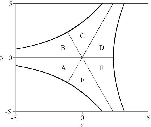
3. This quotient space is two-dimensional and is parameterized byDandk. However, since theSO(3) action is not free, this quotient space is not a manifold. A two-dimensional, totally geodesic manifold which includes the quotient space was introduced in [18]. It is called Y and is the manifold of Nahm data with Ti proportional to σi but with no ordering assumption.
Y is pictured in Figure 1. There are six identical regions labeled A to F. Each is identical to the quotient space but with a different ordering of the top functions. The coordinates on the space are
x = f2 1 +f
2 2 −2f
2 3,
y = √3(f2 2 −f
2
1), (4.21)
so region B corresponds to the orderingf2 1 ≤f
2 2 ≤f
2
3. The thick boundary corresponds to
B
C
A E
D
F
0
-5 5
5
0
-5 y
[image:16.595.171.437.110.333.2]x
Figure 1: The manifold Y.
of the top functions are equal and the corresponding monopole is axially symmetric. This can happen in two ways: eitherk = 0 or k= 1. When k= 0, the (2,[1])-monopole is torus shaped and coincident. This is referred to as the trigonometric case, because the Euler top functions are trigonometric. This is what happens, for example, on the boundary between B and C. When k = 1, the (2,[1])-monopole may separate into two individual monopoles. This is referred to as the hyperbolic case, because the Euler top functions are hyperbolic; for example, on the boundary between B and A:
f1(s) =f2(s) = −DcosechDs
f3(s) = −DcothDs. (4.22)
In this case, the two monopoles separate along the x3-axis. When D is large, it is the separation of the two monopoles [19, 13]. The clouds get bigger as the thick boundary is approached and theα monopoles separate down the legs [18, 19, 17].
The expressions for the ci’s are quite complicated. They are plotted numerically in Figure 2. In this figure, c3 is plotted in regions A and B,c2 in C and F and c1 in D and E. This is done because the top functions are in a different order in each region. Therefore, in each region, a different ci corresponds to each σi. In Figure 2, the ci plotted is the one which corresponds to σ3. The result is a continuous function conY.
c seems to become infinitely large at the boundary. It seems to increase steadily down the CD and EF legs and decrease down the AB leg. This can be confirmed by doing an explicit calculation withk= 1. In this case, it follows from the hyperbolic expressions that
c2 3|k=1 =
(coshDµsinhDµ−Dµ)D DµcoshDµsinhDµ−sinh2
5
0
-5
0
-5 5
y
[image:17.595.172.436.110.336.2]x
Figure 2: A contour plot of cas a potential on Y. The arrow points down the slope.
This has a minimum for infinite D
lim D→∞c
2 3|k=1 =
1
µ. (4.24)
Hence, the potential takes a minimum value for minimum cloud size and maximum sep-aration of the α monopoles. This leads to a critical electric charge which agrees with the string theory (4.38). Similar calculations confirm that c2
1 and c 2
2 diverge as D goes to infinity.
This situation is similar to the (1,[1],1) case discussed in [8]. The uncharged monopole consists of two massive monopoles and a massless one. As described in [13], the SU(2) symmetry acts on the position and charge of the massless monopole. This action moves the massless monopole about on the ellipsoid known as the massless cloud. If the SU(2) symmetry is broken to U(1), the massless β seems to acquire a definite position. The electric 1/4-BPS energy and the electric charge depend also on the position of the massless monopole.
small compared tob, the low energy effective lagrangian is shown to be
L= 1 2
X
p,q
gpq(z) ˙zpz˙q−U(z) (4.25)
where the potential is U(z) = 1
2a·q and so
U(z) =X p,q
1
2gpq(z)(a·K
p)(a·Kq). (4.26)
The potential appears because there are two Higgs fields involved in the 1/4-BPS con-figuration and the electromagnetic force does not exactly cancel the Higgs force. This effective lagrangian is of the order
L∼v2
, ǫ2
(4.27) where v is the order of velocities ˙za and ǫ is the order of |a|/|b|. This lagrangian is valid when v ≪ 1 and ǫ ≪ 1. It has N −1 conserved electric charges, one for each unbroken
U(1) symmetry. There is a BPS bound on this newtonian lagrangian and field theoretic 1/4-BPS configurations appear as BPS configurations.
When ν ≪ µ, the electric contribution to the magnetic energy is small if the electric charge is small. In the (2,[1]) case, the kinetic part of the low energy effective lagrangian is the metric on the space of (2,[1]) monopoles: the Dancer metric [5]. The potential is
U(D, k) = g 2
ν2 2
X
i
c2 in
2
i, (4.28)
that is, one half of the electric 1/4-BPS energy. Since we are considering only the relative motion, there is only one conserved U(1). The position of the β monopole lies on the ellipsoid (4.15). In the trigonometric case k = 1, the massless monopole goes to the infinity when D approaches its maximal value π/µ. In this limit,
fi ≈
π
π−µD (4.29)
and so
c2 i ≈
π
µ(π−µD). (4.30)
Thus, the potential is linearly increasing with the distance from the massless monopole to the twoαmonopoles. Therefore, theβ monopole is confined. In the hyperbolic case, with two massive monopoles well-separated,
f1 =f2 ≈0 (4.31)
and
@ @
@ @@ a
a a a a
(1) (2)
(3) (q,0)
(0, g) (q, g)
t t
t
Figure 3: This is the configuration discussed in [1]. The dots are D3-branes and the lines are strings.
In this limit,
c2 1 =c
2
2 ≈D (4.33)
and
c2
3 = 1/µ. (4.34)
Therefore, if we try to put theβmonopole at the middle of the line connecting two massive
αmonopoles, then the energy increases linearly with the distance. This again implies that the β monopole should be confined to one of the two massive αmonopoles.
4.2
The string theory of the
(2
,
[1])
example
In this subsection, we propose a string configuration corresponding to the (2, [1])-monopole 1/4-BPS state and we justify this proposal with the same sort of marginal stability argument as applied to the (1,1) dyon in [1].
It is believed that 1/4-BPS states correspond to configurations of three-pronged strings [20]. The string configuration given in Figure 3 is a well-understood example [20, 1]. This configuration of strings corresponds, in the field theoretic context, to a (1,1)-monopole with electric charge qα. The string configuration becomes unstable when the (q,0)-string has zero length, that is, when the string junction coincides with the D3-brane labeled (2) in Figure 3.
The tension of a (q, g)-string is pq2+g2 and by balancing the forces at the string junction, it is simple to calculate the angles between the strings [20, 1]. The critical angle at which the (q,0)-string has zero length is easily calculated from the D3-brane positions. This means that the critical electric charge is known. In [1], the covariant Laplace equation (2.2) is solved for (1,1)-monopoles with sufficient explicitness to allow the electric charge to be calculated. It is found that the electric charge has a maximum when the two monopoles are infinitely separated and that this charge is equal to the critical charge calculated from the string theory. Therefore, the critical charge can be calculated from either the string theory or the field theory.
pro-@ @ @ @
t t
t (1)
(2)
(3)
(0,2g) (q, g) (q, g)
(a)
@ @ @ @
t t
t
? 6
ν
µ
θ
[image:20.595.187.425.109.262.2](b)
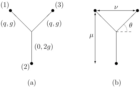
Figure 4: These two pictures are of the Y-shaped string configuration, dots denote D3-branes and lines denote strings. (a) shows which string is which and (b) shows the lengths
µand ν and the angle θ.
posed string configuration is Y-shaped and is shown in Figure 4. The angle θ can be calculated by balancing forces at the junction and is given by
sinθ = p g
q2+g2. (4.35)
This configuration becomes unstable if the (0,2g)-string has zero length and the Y-shape degenerates to the V-shaped configuration illustrated in Figure 5. At the onset of instability
θ =θc (4.36)
where
sinθc =
µ q
1 2ν
2
+µ2
. (4.37)
This means that the critical electric charge is qc where
qc =
gν
2µ. (4.38)
From the string picture it would appear that this critical value of the electric charge is a minimum. This contrasts with the (1,1) case, where the critical value is a maximum. The above value of the critical charge is identical to the charge obtained from (4.20) and (4.24). This critical value corresponds to the 1/4-BPS electric charge of infinitely separated two massive monopoles, with the massless monopole on top of either massive monopole.
Figure 5 might create the suspicion that at some point the Y-shaped configuration has larger energy than the ∇-shaped configuration illustrated in Figure 6. Calculating the energies allays this concern. The V-shaped configuration has energy
EV= 2gµcosec 2
θ = 2gµ(cot2
L L L L L L L L LL
(1)
(2)
(3)
(q, g) (q, g)
θc
t t
[image:21.595.255.361.109.233.2]t
Figure 5: The V-shaped string configuration, this configuration is unstable.
L L L L L L L L LL
t t
t (1)
(2)
(3)
(0, g) (0, g)
(q,0)
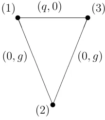
Figure 6: The ∇-shaped string configuration, this configuration appears to have higher energy than the V-shaped configuration.
whereas, the ∇-shaped configuration has energy
E∇= 2gµ(cot2θ+ cosecθ). (4.40)
Therefore,EV≤E∇with equality only ifθis zero orπ/2. Of course, calculations of this sort are an over-simplification but they provide evidence favoring the Y-shaped configuration over the ∇-shaped one.
5
Discussion
In this paper, we have derived a formula for the electric mass and applied it to two examples. There are other examples that might also be considered. It would be simple to extend the analysis to the (2,1)-monopole, in which theβ monopole has a magnetic mass. In this case, the gauge orthogonality conditions require [13]
[image:21.595.254.362.276.400.2]use the numerical ADHMN construction of [24] to find the a field. This would reveal the spatial distribution of the electric mass. This might be interesting in examples, like the one considered in this paper, where there are monopoles with no magnetic mass. It would also be instructive in examples, such as those in [23], where there are extra minima of the Higgs field.
The dynamics of 1/4-BPS states are not fully understood. In the better understood (1,1) example the level set of the potential lies on a group orbit. In the (2,[1]) example, this is not the case as there are monopoles with the same electric mass which cannot be group transformed into each other. The geodesic motion on the Y space was studied by Dancer and Leese [18]. It would be interesting to determine how this motion is modified by the presence of the potential.
Acknowledgment
CJH warmly thanks the Physics Department and Center for Theoretical Physics, Seoul National University for hospitality while part of this work was undertaken. CJH thanks Fitzwilliam College, Cambridge for a research fellowship and thanks Patrick Irwin and Paul Sutcliffe for useful discussion. KL appreciates the Aspen Center for Physics, Columbia University and PIMS of University of British Columbia for support and hospitality. KL is supported in part by the SRC program of SNU-CTP, the Basic Science and Research Program under BRSI-98-2418, and KOSEF 1998 Interdisciplinary Research Grant 98-07-02-07-01-5.
References
[1] K. Lee and P. Yi, Phys. Rev. D 58 (1998) 066005, hep-th/9804174.
[2] D. Bak, K. Hashimoto, B.-H. Lee, H. Min and N. Sasakura, Phys. Rev. D 60 (1999) 046005, hep-th/9901107; K. Hashimoto, H. Hata and N. Sasakura, Phys. Lett. B 431 (1998) 303, hep-th/9803127; Nucl.Phys. B535 ((1998) 83, hep-th/9804164; T. Kawano and K. Okuyama, Phys. Lett. B 432 (1998) 338, hep-th/9804139.
[3] T. Ioannidou and P.M. Sutcliffe, Phys. Lett. B 467 (1999) 54. hep-th/9907157. [4] D. Tong, Phys. Lett. B 460 (1999) 295, hep-th/9902005.
[5] A.S. Dancer, Commun. Math. Phys. 158 (1993) 545. [6] A.S. Dancer, Nonlinearity 5 (1992) 1355.
[9] D. Bak, C. Lee, K. Lee and P. Yi, Phys. Rev. D 61 (2000) 025001, hep-th/9906119. [10] E.J. Weinberg, Nucl. Phys. B167 (1980) 500; Nucl. Phys. B 203 (1982) 445.
[11] W. Nahm,The construction of all self-dual multimonopoles by the ADHM methodin Monopoles in quantum field theory edited by N.S. Craigie, P. Goddard and W. Nahm (World Scientific, Singapore, 1982).
[12] N.J. Hitchin, Commun. Math. Phys. 89 (1983) 145.
[13] C.J. Houghton, P. Irwin and A.J. Mountain, JHEP 9904 (1999) 029,hep-th/9902111. [14] T.C. Kraan and P. van Baal, Phys. Lett. B 428 (1998) 268, hep-th/9802049.
[15] H. Osborn, Ann. Phys. (N.Y.) 135 (1981) 373.
[16] H. Nakajima, Monopoles and Nahm’s equations in Einstein metrics and Yang-Mills connections edited by T. Mabuchi and S. Mukai (Marcel Dekker, New York, 1993). [17] P. Irwin, Phys. Rev. D 56 (1997) 5200, hep-th/9704153.
[18] A.S. Dancer and R.A. Leese, Proc. R. Soc. Lond. A 440 (1993) 421. [19] A.S. Dancer and R.A. Leese, Phys. Lett. 390B (1997) 252.
[20] O. Bergman, Nucl. Phys. B525 (1998) 104, hep-th/9712211. [21] C.J. Houghton, Phys. Rev. D 56 (1997) 1220,hep-th/9702161. [22] K. Lee and C. Lu, Phys. Rev. D 57 (1998) 5260, hep-th/9709080.
[23] C.J. Houghton and P.M. Sutcliffe, J. Maths. Phys. 38 (1997) 5576,hep-th/9708006. [24] C.J. Houghton and P.M. Sutcliffe, Commun. Math. Phys. 180 (1996) 343,