The effects of disorder in strongly interacting quantum systems

(1)

THE EFFECTS OF DISORDER IN STRONGLY

INTERACTING QUANTUM SYSTEMS

Steven J. Thomson

A Thesis Submitted for the Degree of PhD at the

University of St Andrews

2016

Full metadata for this item is available in St Andrews Research Repository

at:

http://research-repository.st-andrews.ac.uk/

Please use this identifier to cite or link to this item: http://hdl.handle.net/10023/9441

(2)

The E

↵

ects of Disorder in Strongly

Interacting Quantum Systems

Steven J. Thomson

This thesis is submitted in partial fulfilment for the degree

of PhD at the University of St Andrews

(3)

(4)

1. Candidate’s declarations:

I, Steven Thomson, hereby certify that this thesis, which is approximately 43,000 words in length, has been written by me, and that it is the record of work carried out by me, or principally by myself in collaboration with others as acknowledged, and that it has not been submitted in any previous application for a higher degree.

I was admitted as a research student in August 2012 and as a candidate for the degree of PhD in August 2012; the higher study for which this is a record was carried out in the University of St Andrews between 2012 and 2016.

Date ……….. Signature of candidate ………. 2. Supervisor’s declaration:

I hereby certify that the candidate has fulfilled the conditions of the Resolution and Regulations

appropriate for the degree of ……… in the University of St Andrews and that the candidate is qualified to submit this thesis in application for that degree.

Date ……….. Signature of supervisor ……….

3. Permission for publication: (to be signed by both candidate and supervisor)

In submitting this thesis to the University of St Andrews I understand that I am giving permission for it to be made available for use in accordance with the regulations of the University Library for the time being in force, subject to any copyright vested in the work not being affected thereby. I also

understand that the title and the abstract will be published, and that a copy of the work may be made and supplied to any bona fide library or research worker, that my thesis will be electronically

accessible for personal or research use unless exempt by award of an embargo as requested below, and that the library has the right to migrate my thesis into new electronic forms as required to ensure continued access to the thesis. I have obtained any third-party copyright permissions that may be required in order to allow such access and migration, or have requested the appropriate embargo below.

The following is an agreed request by candidate and supervisor regarding the publication of this thesis:

PRINTED COPY

a) No embargo on print copy

ELECTRONIC COPY

a) No embargo on electronic copy b)

(5)

(6)

For my parents, whose unwavering support and encouragement has enabled me to get this far. I know you probably won’t understand a word of this thesis, but I

(7)

(8)

Abstract

This thesis contains four studies of the e↵ects of disorder and randomness on strongly correlated quantum phases of matter. Starting with an itinerant ferromagnet, I first use an order-by-disorder approach to show that adding quenched charged disorder to the model generates new quantum fluctuations in the vicinity of the quantum critical point which lead to the formation of a novel magnetic phase known as a helical glass.

Switching to bosons, I then employ a momentum-shell renormalisation group analysis of disordered lattice gases of bosons where I show that disorder breaks ergodicity in a non-trivial way, leading to unexpected glassy freezing e↵ects. This work was carried out in the context of ultracold atomic gases, however the same physics can be realised in dimerised quantum antiferromagnets. By mapping the antiferromagnetic model onto a hard-core lattice gas of bosons, I go on to show the importance of the non-ergodic e↵ects to the thermodynamics of the model and find evidence for an unusual glassy phase known as a Mott glass not previously thought to exist in this model.

Finally, I use a mean-field numerical approach to simulate current generation quantum gas microscopes and demonstrate the feasibility of a novel measurement scheme designed to measure the Edwards-Anderson order parameter, a quantity which describes the degree of ergodicity breaking and which has never before been experimentally measured in any strongly correlated quantum system.

(9)

(10)

Acknowledgements

First and foremost, I’d like to thank my supervisors, Frank Kruger¨ and

Chris Hooley for taking me on as a PhD student and for all their advice and support over the last four years. I’d also like to thank the Condensed Matter Doctoral Training Centre and in particular acknowledge the eternal debt that all its students owe toChristine Edwards, Julie Masseyand Wendy Clark for everything they’ve done on behalf of all of the students and sta↵members in the Centre.

I’ve had the tremendous good fortune to share an office with some excellent officemates and friends. I’d like to thank Calum Lithgowfor teaching me more about politics and grammar than I ever wanted to know, but also for educating me about whisky, and Helen Cammack for never letting me forget that there can be more to life than equations. I endeavour to one day figure out just what she’s talking about. I’d also like to thankScott Pearsonfor his hard-won advice and wisdom that’s been so much help to me over the years.

All of the sta↵ and students of the School of Physics & Astronomy deserve more thanks than I can possibily articulate. In particular, thanks to Jonathan Keelingfor his help and advice, toGraham Bruce for trusting my crazy ideas and to Liam Walker for choosing to work with us for his Masters project, as well as to our collaboratorTi↵any Hartefor her invaluable contributions to that work. During the last few years, I’ve also benefited greatly from opportunities to talk with many others from outwith St Andrews and in particular I’d like to thank Andrew Green and Chris Pedder for useful conversations and advice. I particularly wish to thank my examiners,Brendon Lovettand Joe Bhaseen

for investing their time in reading my thesis and o↵ering useful comments, as well as for making the viva one of the definite highlights of my PhD.

(11)

And as I have learned my teachers, so too have I learned from my students. To all of you whom I’ve taught over the years - I suspect I’ve learned at least as much from you as you’ve learned from me and I’d like to thank you all for being the most fantastic bunch of students I could have hoped for. I hope my tutoring hasn’t left you with any lasting trauma.

To all my friends outside the School, both in St Andrews and elsewhere, without whom I’d have never managed to emerge from the PhD as anything resembling a functioning human being. To the sta↵ of the local bottle shops and bars, without whom I may not have coped. To whoever invented co↵ee. To my family for believing in me. To the ghosts and the poets, to the lost and the free.

Were I not the type to use five hundred and eighty five words where nineteen would suffice, I could have summed up all of the above in a single sentence:

(12)

“It’s the questions we can’t answer that teach us the most. They teach us how to think...The harder the question, the harder we hunt. The harder we hunt, the

more we learn. An impossible question...”

(13)

(14)

Chapter 1 Introduction

Nothing in life is perfect and what’s true in life is true for quantum materials. Randomness and disorder are present to some degree in every substance in the world, despite every e↵ort to create the cleanest, purest materials possible. Even small concentrations of impurities in quantum materials can dramatically alter their properties, for better or for worse.

Since the time of the Crusades, blacksmiths have known that introducing controlled carbon impurities into swords could vastly improve the properties of the blade, leading to the development of the famed Damascus steel. Stronger than any contemporary materials, Damascus steel was later found to contain carbon nanotubes [1], making it arguably the first commercial application of nanotechnology. We now know that doping materials can lead to the emergence of dramatic properties such as superconductivity [2]. Understanding the e↵ects of disorder is crucial to the continued development of materials and technology but is also important for our understanding of the underlying physics in strongly interacting quantum systems. Disorder and impurities often act as excellent probes of quantum behaviour, changing the properties of the system in question in measurable ways and giving us valuable information as to the underlying physics.

(17)

1.1 Classical Phase Transitions

A phase transition is the process by which a thermodynamically large number of interacting particles collectively change their state of matter, e.g. from liquid to solid, liquid to gas, magnetic to non-magnetic or a vast number of other possibilities.

Classical phase transitions occur at finite temperature, where the transfor-mation between phases is driven by thermal fluctuations. Consequently, they are also known as ‘thermal transitions’. At a classical phase transition, the dynamic and static behaviour of the system decouple from each other and the transition can be described by a time-independent theory.

Many phase transitions are accompanied by a breaking of some fundamental symmetry of the system and a corresponding change in how ordered the material is. Transitions are driven by the competition between energy and entropy as the system tries to minimise its Helmholtz free energy _F = E T S, where E is the internal energy of the system, T is temperature and S is entropy. At low temperatures, the entropic term has a negligible e↵ect and so the system adopts a configuration that minimises its internal energy, which tend to be highly ordered states with broken symmetries. At higher temperatures, the system will transition into a state where it instead maximises its entropy S, which tend to be more isotropic and symmetrical configurations. For example, in the case of liquid water, as the temperature is lowered the isotropic, symmetric liquid (large entropy) freezes into a highly ordered (low entropy) sixfold-symmetric crystal lattice where the rotational symmetry of the liquid is broken in favour of the hexagonal symmetry of ice1_.

This picture is largely generic, though there are some phase transitions where the nature of the symmetry breaking present (if any) remains ambiguous [3–5] and others which don’t break any symmetries at all, such as liquid water into water vapour or the Kosterlitz-Thouless transition [6] seen in the two dimensional XY model.

Phase transitions typically fall into two main classes: the discontinuous first-order transitions and the continuous second-order transitions. First order transitions carry with them discontinuities in entropy and a latent heat, whereas second order transitions do not. In general, annth_{order transition is characterised}

by a discontinuity in the nth _{derivative of the free energy, however this is not}

considered a rigorous definition [7] as some derivatives of the free energy diverge on approach to a phase transition, e.g. specific heat in ferromagnets.

The nature of a transition is not immutable and can change for di↵erent values of external parameters such as temperature, pressure, applied magnetic

1_{There are at least sixteen other distinct types of ice crystal existing under a variety of}

conditions which display di↵erent forms of ordering, but the hexagonal crystalline ice 1his the

(18)

[image:18.595.164.455.57.327.2]

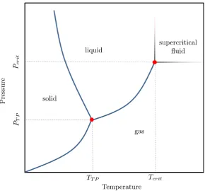
Figure 1.1 A schematic phase diagram of water in the temperature-pressure plane showing the approximate regions where each phase occurs. The blue lines represent phase transitions. The lower red dot is the triple point at which all three phases can co-exist. The upper red dot is the critical point where the first-order liquid to gas transition terminates and becomes second order. Above this point there is no distinct liquid-to-gas transition and instead a so-called supercritical fluid exists in this parameter regime.

(19)

1.2 Landau Theory

Almost every phase transition has an order parameter that defines where the transition takes place. This is some quantity that has a thermodynamic average of zero in the disordered phase and takes on some finite value in the ordered phase. Near a second-order or weakly first-order phase transition, we can assume that the order parameter is small.

The key idea behind Landau theory is that the free energy near a transition can be Taylor expanded in powers of the order parameter. Implicitly, this assumes the free energy to be analytic in the order parameter. For this description to be physical, the free energy must obey the same symmetries as the Hamiltonian. In practice, this typically leads to only even powers of the order parameter featuring in the expansion. More generally, any term in the expansion that explicitly breaks any symmetry in the initial Hamiltonian will be absent.

As an illustrative example, let us consider expanding some generic free energy

F in even powers of some order parameterm like so:

F =↵m2+ m4+ m6+... (1.1)

where the coefficients↵, and are all functions of the microscopic parameters of the system in question. The coefficient of the final term in the expansion must always be positive or else the free energy becomes unbounded from below, which is unphysical.

If ↵, and are all positive then the free energy is minimised by m = 0. If ↵ < 0 and > 0 then is not needed and we see that the free energy is minimised by a non-zero m = _±p_|↵_|/2 . The transition is given by ↵ = 0, i.e. the line along which a non-zerom becomes favoured. As↵turns from positive to negative, F develops two minima which emerge smoothly from m= 0, shown in Fig. 1.2. The ground state magnetisation continuously increases from zero and this is a second-order phase transition.

This formalism can also describe first-order phase transitions. Consider the case of ↵ > 0, > 0 but < 0, also shown in Fig. 1.2. We see that the free energy now acquires two local minima at somem6= 0. If is sufficiently negative (specifically, if < 0 and 2 ₄_↵ _{) then these minima will drop below the}

(20)

Figure 1.2 Schematic free energy diagrams. i) A second-order transition as ↵ goes from positive to negative, with minima located at m ₆= 0

smoothly moving out from the centre. ii) A first-order transition where becomes sufficiently negative that the two local minima shown in black dip below them= 0 minimum and the magnetisation abruptly jumps from m= 0 to some non-zero m.

1.3 Correlation Length

Approaching the critical point at which a second-order phase transition occurs, fluctuations of the order parameter on larger and larger length scales become increasingly important. These are known as critical fluctuations. In the vicinity of a critical point there is only one physically relevant length scale, known as the correlation length, which is the largest length scale on which the order parameter fluctuations occur and takes the following form:

⇠ / T Tc

Tc

⌫

, (1.2)

where Tc is the critical temperature at which the phase transition occurs and ⌫

is known as the correlation length exponent.

Close to the phase transition, the correlation length diverges. It becomes the largest length scale in the system and consequently the only relevant one for determining the properties of the system. The system e↵ectively self-averages over large volumes, in other words, and small microscopic fluctuations become unimportant as only large-scale properties such as dimensionality and lattice geometry a↵ect the overall behaviour.

(21)

detailed microscopics of the system as they can only cause quantitative changes.

The diverging correlation length close to a critical point is also responsible for the phenomenon of critical opalescence, where a normally transparent liquid will turn opaque when the correlation length becomes comparable to the wavelength of light, leading to the scattering of light and causing the liquid to take on a cloudy white appearance. This is a dramatic and very visual demonstration of the diverging correlation length that occurs near a classical critical point.

1.4 Quantum Phase Transitions

Classical phase transitions are driven solely by thermal fluctuations. If we cool down our system to T = 0, then, does that mean we end up in a fluctuationless ground state that exhibits no phase transitions? Classical theory alone would have us believe so, but quantum theory tells us that such a fluctuationless state is impossible. Driven by the Heisenberg uncertainty principle, even a system in its ground state at T = 0 will exhibit quantum mechanical fluctuations that, in combination with the tuning of some non-thermal physical parameter, can lead to so-called quantum phase transitions. For T >0, even if the phases themselves require a quantum mechanical description (such as superfluidity or superconductivity), the transition into and out of the phase is still a classical phase transition in which quantum mechanics plays no role.

Quantum phase transitions [8] di↵er from the classical phase transitions described earlier in that the kinetic and potential parts of the Hamiltonian do not commute, meaning the partition function does not factorise. Static and dynamic behaviour no longer decouple and must be treated on an equal footing, leading to not only a divergent correlation length in space, but also a divergent correlation time.

At zero temperature, the correlation length can be expressed in a similar form as Eq. 1.2 but with some non-thermal quantityg taking the place of temperature:

⇠ _/ g gc

gc

⌫

, (1.3)

where g is some parameter such as pressure or applied magnetic field and gc is

the critical value of this parameter at which the phase transition occurs. The correlation time is given by:

tC /

g gc

gc

dz⌫

. (1.4)

where dz is the dynamical critical exponent. It is also commonly denoted z,

however in this thesis we shall use dz for the dynamical critical exponent and

(22)

The necessity of treating space and time on an equal footing introduces additional dimensions to what was previously a time-independent problem and means that quantum phase transitions in d dimensions may often be mapped onto classical phase transitions in d+dz dimensions.

Ifdz = 1 then the relevant correlation functions scale the same in each spatial

dimension as they do in time. This is often not true for quantum critical points, and for dz 6= 1 we end up with a theory where space and time scale di↵erently,

leading to quantum critical points exhibiting much richer behaviour than simply being a classical critical point in ‘more dimensions’.

A divergent correlation time is not the only extra consideration we need make in describing a quantum phase transition. The real distinguishing feature of a quantum phase transition is that it occurs at zero temperature, but it turns out that we can incorporate both real time and temperature together in a single move.

Imaginary time

In classical statistical mechanics, Boltzmann weightings are given by terms of the form e Hˆ where ˆH is the Hamiltonian and = 1/kBT is the inverse

temperature. In quantum mechanics, evolution in real time is given by e iHˆt/~_.

In order to perform quantum statistical mechanics, we can make a Wick rotation from real time to imaginary time t ! i⌧ where ⌧ 2 [0,~ ] such that we can describe these thermal weightings in terms of imaginary time. This allows us to construct partition functions as path integrals over an imaginary time dimension of length ~ . The mapping takes the form:

Z = Tr⇥e H⇤ (1.5)

=

Z

D[ ⇤, ] exp

Z _~

0

d⌧ ( ⇤@⌧ H) , (1.6)

where the rewriting in terms of a path integral over bosonic coherent states is as shown in Ref. [9]. This representation allows us to treat both real-time dynamics and quantum statistics at the same time. At zero temperature, the length of the imaginary time dimension is infinite and its contribution can be treated on an equal footing with the spatial dimensions. At non-zero temperatures, the length of the imaginary time dimension is finite. The quantum-to-classical mapping can then lead to classical systems with odd geometries, being infinite in extent in d dimensions and finite in dz.

(23)

of critical phenomena not seen in classical systems. For fermions, the mapping can even generate negative Boltzmann weights - this is known as the fermion sign problem, and is one of the major problems facing modern condensed matter physics. (It is in the complexity class NP-hard [12], which is featured in the Clay Mathematics Institute’s Millennium Prize Problems with a$1 million prize for a solution [13].)

Given that the length of the imaginary time dimension is infinite only atT = 0 and that the quantum phase transition itself only occurs at zero temperature, one might wonder whether the imaginary time dependence can be neglected whenever ~ is finite and a purely classical description used for all but the extremeT = 0 case. This turns out not to be the case: although the quantum phase transition itself is restricted to T = 0, there is a large region at finite temperatures where quantum fluctuations originating at zero-temperature quantum critical points turn out to be extremely important.

1.5 Quantum Criticality

Despite quantum phase transitions strictly only taking place at T = 0, their e↵ects may still be felt at finite2 _{temperatures. From the correlation time} _t

c

it follows that we can define a corresponding quantum fluctuation frequency !. Consider a system at temperature kBT with some generic quantum fluctuations

of strength ~!. When~! kBT then the system will undergo a quantum phase

transition. Conversely, for kBT ~!, the system will undergo a classical phase

transition. This criterion will always be satisfied sufficiently close to the transition for any T > 0 and the transition will always be classical in nature, even if the phases themselves require a quantum mechanical description.

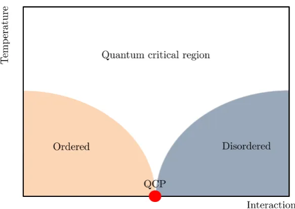
There is, however, a region of the phase diagram where the quantum and thermal fluctuations are approximately equal in size. Plotting the boundaries defined by ~! _⇡ kBT defines the so-called quantum critical region: a roughly

conical region extending out from theT = 0 quantum critical point. A schematic phase diagram is shown in Fig. 1.3. Within this region, the e↵ects of quantum fluctuations are strongly felt and the behaviour of the system will not be classical. For example, Fermi liquid theory [9] will not apply in this region even for an ‘ideal’ metal due to the presence of these strong quantum fluctuations [14].

These quantum fluctuations can lead to all sorts of interesting behaviour. Experimentally, second-order phase transitions are commonly seen to turn first-order in the vicinity of QCPs in a variety of materials [15–19], and often entirely new phases are found. Examples of this include the superconductivity seen in UGe2 [20–23], the modulated nematic phase seen in Sr3Ru2O7 [24–27], the

partially-ordered phase seen in MnSi [28, 29] and the modulated spiral seen in

2_{Following Ref. [8], I engage in the same ‘almost standard abuse of language’ and refer to}

(24)

[image:24.595.164.456.63.270.2]

Figure 1.3 Schematic phase diagram showing quantum ordered, quantum disordered and quantum critical regions. The quantum critical point (QCP) is indicated in red. Above it, the roughly-conical region where critical fluctuations strongly influence the behaviour of the material extends up to non-zero temperatures.

PrPtAl [30], to name but a few.

It is this fluctuation-dominated region that makes the study of quantum phase transitions both useful and interesting. The extended e↵ects of quantum fluctuations beyond the strictly zero-temperature limit means that understanding the role of quantum fluctuations at zero temperature can still tell us useful information about the finite-temperature response of the material.

(25)

1.6 Universal Behaviour

Due to the diverging correlation length and the power-law behaviour assumed by various thermodynamic quantities (such as the specific heat, correlation length, order parameter scaling and susceptibility, to name but a few), the behaviour of a system in the vicinity of a second-order phase transition can be completely described by a set of numbers known as critical exponents. Similar to the correlation length exponent ⌫, each of these thermodynamic quantities has a corresponding critical exponent. These are shown in Table 1.1.

Common critical exponents

specific heat C⇠| |↵

magnetisation M ⇠| |

magnetic susceptibility _⇠_{| |}

field dependence of M M _⇠_|(h hc)/hc|1/

spatial correlation length ⇠⇠| | ⌫

temporal correlation length ⌧ ⇠⇠dz ₌_{| |} dz⌫

Table 1.1 A list of common thermodynamic quantities and how they scale with their critical exponents, where = (T Tc)/Tc in the classical case

and = (g gc)/gc in the quantum case. In the fourth line, h is the

external magnetic field. Information from Ref. [9].

The last entry of Table 1.1 shows the role that the dynamical critical exponent dz plays in the relation between the temporal correlation length⌧ and the spatial

correlation length ⇠ and illustrates the extra e↵ective dimensionality of T = 0 quantum systems.

The di↵erent critical exponents are related to one another through the scaling relations shown in Table 1.2, where most of the exponents are as shown in Table 1.1 and ⌘ is the anomalous dimension of the correlation function, defined by the scaling form:

C(r)⇠

⇢ 1

|r|d 2+⌘ |r|⌧⇠

exp( _|r_|/⇠) _|r_| ⇠ . (1.7)

This expression reflects that the correlation function changes from exponential to power-law scaling at the length scale ⇠ given by the correlation length. In other words, when ⇠ diverges at the critical point, we move from short-ranged exponential decay to long-range power-law correlations. This is only strictly true at the critical point: even in the ordered phase, the connected correlation function need not display power-law decay. Its precise form depends on the excitation spectrum of the system in question.

(26)

Scaling laws

Fisher ⌫(2 ⌘) =

Rushbrooke ↵+ 2 + = 2

Widom ( 1) =

[image:26.595.161.478.56.130.2]

Josephson 2 ↵=⌫d

Table 1.2 Scaling laws. Information from Ref. [9]. The final relation is the only one to involve the spatial dimension and is known as a hyperscaling relation. Hyperscaling does not hold in d >4 when mean-field theory becomes exact and the correlation length exponent no longer has any dependence on spatial dimensionality.

Table of critical exponents

↵ ⌫

d= 2 Ising 0 1/8 1/4 15 1

d= 3 Ising 0.110(1) 0.6265(2) 1.2372(5) 4.789(2) 0.6301(4) d= 3 XY 0.0146(8) 0.3485(2) 1.3177(5) 4.780(2) 0.67155(27) d= 3 Heisenberg -0.122(9) 0.3662(25) 1.390(5) 4.796(1) 0.7073(30)

d= 4 Ising 0 1/2 1 3 1/2

Table 1.3 An illustrative and non-exhaustive list of calculated critical exponents for a variety of di↵erent universality classes. The numerical values were sourced from Refs. [32–34] and the numbers in brackets indicate the uncertainty in the final digit. The d= 4Ising results are exactly given by mean-field theory. Wherever any particular exponents were not given in the references they were calculated from the ones given using the scaling relations listed in Table 1.2 and the uncertainties propagated in the standard manner.

given system. To illustrate this, Table 1.3 shows a selection of critical exponents for a variety of di↵erent models in di↵erent dimensions. Within the uncertainties, it is possible to use the scaling relations in Table 1.2 to calculate any exponent from any other two. (The uncertainties listed are in most cases the result of direct calculation from the sources referenced. Consequently they may be smaller than the resulting uncertainties obtained if one calculates the exponent from others listed and propagates their errors accordingly.)

Since the critical exponents are determined from fundamental underlying physics rather than microscopic details, often very di↵erent physical systems display the same set of critical exponents. These sets of critical exponents are called universality classes.

(27)

physical system depended critically on its specific microscopic structure, much of the predictive power of condensed matter theory would be lost. The ability to instead pick out the most relevant pieces of the underlying physics and discard the irrelevant degrees of freedom is what allows our models to be so general, not to mention one of the main reasons they are mathematically tractable to begin with.

1.7 Renormalisation Group

Arising directly from the idea of focusing only on the most relevant underlying physics, the main technique we will employ in Chapters 3 and 4 is the renormalisation group, a powerful analytical technique allowing us to ‘zoom out’ from our microscopic picture of individual quantum particles and instead examine the global behaviour of a thermodynamically large system. Renormalisation works because of the diverging correlation length in the vicinity of quantum critical points, allowing us to eliminate the short wavelength non-universal degrees of freedom in order to obtain a description of the system entirely in terms of the long-wavelength universal modes which determine its bulk behaviour. Initially employed in the context of quantum electrodynamics [35], the renormalisation group in its condensed matter form was developed in Refs. [36, 37] and has since become one of the most important tools used in condensed matter theory.

Essentially, renormalisation is a technique used to move away from a micro-scopic picture to a macromicro-scopic one in a procedure of ‘controllably forgetting’ about the high energy, short wavelength degrees of freedom. Formally, we typically define a cuto↵ length or energy scale and integrate out the modes which we are not interested in, thereby leaving an action ostensibly in terms of (for example) the long wavelength, low energy modes but that has still taken the higher energy fluctuations into account. See Refs. [38, 39] for a full and comprehensive review of renormalisation group techniques.

In a renormalisable system, variables fall into three main categories. A ‘relevant’ variable is one which grows in magnitude as we zoom out, and therefore is important to the long-wavelength behaviour of the system. Conversely, an ‘irrelevant’ variable is one that renormalises to zero, indicating that it has no bearing on the long-wavelength behaviour which we are interested in (though it can contribute quantitative corrections). In between these two extremes, a variable that does not scale at all under the renormalisation group process is called ‘marginal’ since it isn’t clear from a simple scaling argument whether or not it is important to the physics we are interested in. By tracking how these variables evolve under the renormalisation group process (the renormalisation group flow), we can calculate the long-wavelength behaviour of the model.

(28)

the inverse power of a variable ⇤ then although ⇤ may itself be irrelevant, it must be retained in the theory in order to properly account for the behaviour of . These variables are known as ‘dangerously irrelevant’ and contribute to the leading scaling behaviour despite being themselves irrelevant.

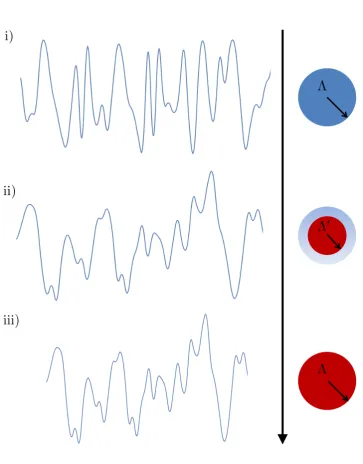
Fig. 1.4 shows a cartoon representation of the renormalisation group process. Panel i) shows an initial field, panel ii) shows the integration over the high frequency components (here performed with a low-pass filter) and panel iii) shows the final rescaling such that the final ‘renormalised’ field resembles the initial field except that it now contains fewer degrees of freedom.

A key assumption of renormalisation group is that one is free to integrate out the short-wavelength, high energy modes independently of the long wavelength universal behaviour of the system. In a disordered system, this assumption is not necessarily valid [41], as we shall see later. In strongly disordered systems, the short-wavelength behaviour can implicitly depend on the long-wavelength behaviour and care must be taken to implement the renormalisation group procedure properly.

The ‘zooming out’ procedure may equivalently be performed in real space or in momentum-space [40], and renormalisation more generally can also be applied in other frameworks such as density matrix renormalisation group [42, 43]. In this thesis, we focus on momentum-shell renormalisation group where we integrate out infinitesimal shells of highest momenta modes and compute the e↵ect they have on the remaining lower-momenta modes. With that in mind, we shall specialise to momentum-shell renormalisation group and look at an example calculation.

Momentum-Shell Renormalisation Group

Beginning from a partition function defined in terms of some field in the following way:

Z =

Z

D[ ]e S[ ], (1.8)

we can split the field into ‘fast’ high momentum fields > and ‘slow’

low-momentum fields < such that

= <+ >. (1.9)

We may then integrate out the fast fields by writing the partition function in the following form:

Z =

Z

D[ <]D[ >]e S[ <, >]. (1.10)

(29)

[image:29.595.94.458.56.521.2]

(30)

between the fast and the slow fields, they can be integrated out independently of one another but in general the fast and slow fields will be mixed. We can write our action as a ‘fast’ action, a ‘slow’ action and a contribution which mixes the fast and slow fields:

S[ <, >] =S0[ <] +S1[ >] + S[ <, >], (1.11)

such that we can write:

Ae S˜[ <]_{= e} S0[ <] Z

D[ >]e S1[ >]e S (1.12)

= e S0[ <]_h_e S_i

S1[ >], (1.13)

whereA is some unimportant constant and we compute the average with respect to S1[ >]. Treating this term perturbatively, we may write:

⌦

e S[ ]↵_S 1[ >]⇡

⌧

1 S+ 1 2( S)

2 ₊_... _(1.14)

= 1 _h S_i+1 2h S

2

i (1.15)

= exp

✓

ln (1 h Si+ 1 2h S

2_i₎

◆

(1.16)

⇡exp

✓

h Si+ 1 2(h S

2_i _h _S_i2₎

◆

. (1.17)

All that remains is to calculate the averages. Following the established paradigm of momentum-shell renormalisation group, we do this using Wick’s theorem. This requires that the ‘bare’ action be quadratic in the fields and we treat any higher-order terms perturbatively.

After evaluating the averages and re-exponentiating the remaining ‘slow’ field terms, we arrive at some new e↵ective action ˜S[ <]. The system is renormalisable

if ˜S[ <] takes the same functional form as the initial action. It is remarkable that

so many physical systems turn out to be renormalisable in this sense.

We then rescale to get back the ‘resolution’ lost by integrating out this momentum shell (shown schematically in Fig. 1.4 going from panel b) to panel c)), and this allows us to derive a set of RG equations showing us how the coefficients of the terms in the action change as we successively integrate out more infinitesimally thin shells. By studying these equations, we can find the scale-invariant fixed points that determine the collective behaviour of the system.

Gaussian Model

(31)

of the fast and slow fields (i.e. S= 0) and all the integrals are Gaussian.

S =

Z 1

0

(ck2+r) ¯ dk. (1.18)

We can split the fields into fast and slow as described previously and integrate out the fast fields exactly to obtain an action of the following form:

˜ S =

Z e dl

0

(ck2+r) ¯ dk. (1.19)

We then want to rescale so the integration range is restored from 0 to 1, and we want to make the rescaling such that the k2 _{prefactor remains unchanged. This}

corresponds to the transformations

k!kedl, (1.20)

| |2 _!_e dl_| _|2_, _(1.21)

and we then choose such that the prefactor of k2 _{remains unchanged. Under}

this rescaling the mass term r becomes:

r!re2dl ⇡r(1 + 2dl), (1.22)

and we can finally write down the renormalisation group equation forrdescribing how it scales with l:

dr

dl = 2r. (1.23)

(32)

Fixed Points

The Gaussian model in the preceding section is exactly solvable but contains no interesting behaviour. In general, there will be cross-couplings between fast and slow fields and an RG equation will take the form F0_{(l) =}_↵_F_{(l) +} _where the ↵ refers to the tree level scaling and the is the renormalisation due to the coupling between fast and slow fields. If ↵ > 0 then the variable F(l) will initially increase under RG, i.e. it is a relevant variable. Similarly, ↵<0 defines an irrelevant variable which will renormalise to 0. In the case of ↵ = 0 the variable is marginal and does not scale under the RG - the higher-order vertex contributions (i.e. the terms) must then be computed to determine whether the variable has any e↵ect at all on the macroscopic behaviour of the system. The terms have a more important role than this, however - they can also give rise to non-trivial fixed points where F0_{(l) = 0 which allow us to determine the} behaviour of the system.

Once we have a set of renormalisation group equations for all running variables in the problem, we can solve them simultaneously for all the points F0_{(l) = 0 to obtain the points in parameter space which are stable under} the renormalisation group flow. These are known as fixed points, as if the running variables take precisely these values they will not change under the renormalisation group process. In practice, the variables will never take precisely the fixed-point values but will approach them asymptotically. As the variables flow closer to the fixed point values, the system begins to look the same at all length scales, a property known as scale invariance. The most famous examples of scale invariance are fractals, as shown in Fig. 1.5, where any arbitrarily small sub-region contains the full information of the entire system.

In Section 1.3 we saw that we can always define a correlation length of a system. The existence of a well-defined dominant length scale does not naturally fit with the idea of scale-invariance exhibited at the renormalisation group fixed points. This implies that at the fixed point, either the correlation length is zero, or it is infinite. In the vicinity of a second-order phase transition the correlation length will diverge, and therefore we can identify the renormalisation group fixed points as potentially indicative of second-order phase transitions.

Following the relevant/irrelevant/marginal classification of variables under the renormalisation group process, the fixed points come in three di↵erent types:

• Stable fixed points where all variables are either irrelevant or marginal. These fixed points are attractive and correspond to stable phases.

(33)

Figure 1.5 The Sierpinski triangle, a fractal which repeats indefinitely as one zooms in. Each small subsection contains the complete information about the full structure. This is a dramatic example of scale-invariance (or ‘self-similarity’).

the same sense that one can balance a pencil on its sharp end - technically valid but physically unrealisable.

• Generic fixed points with a mixture of relevant and irrelevant variables. These correspond to transitions between phases and act to drive the system towards stable fixed points corresponding to stable phases.

Solving the set of renormalisation group equations for all the variables in the problem thus allows us to find out what possible phases the model can adopt and describe the transitions into and out of those phases. This is the goal of a renormalisation group study of any system - the establishment and investigation of the fixed points.

The principles of scale invariance and universality lead to the renormalisation group being an enormously powerful method with which to investigate strongly correlated quantum systems. But what happens when we are no longer dealing with pristine, pure materials but instead consider the addition of disorder - how can we hope to systematically investigate randomness?

1.8 Disordered Systems

(34)

impurities through to significant inhomogeneities that can drastically change the properties of the material. Experimentally, even the purest of samples can display important disorder-induced e↵ects, and that’s not even to mention the materials which are deliberately doped or disordered in an e↵ort to modify their properties.

Even more so than classical systems, quantum materials can exhibit extreme sensitivity to the addition of disorder. Sometimes this disorder can be advan-tageous, as in the case of the doped cuprates [2, 44–47] and pnictides [48–51] where doping can induce superconductivity, but other times it can destroy the very features we’re interested in, such as in Sr2RuO4 [52] where disorder rapidly

suppresses the superconducting critical temperature.

The way a material responds to disorder can tell us something about the physics of the clean system, such as in the case of Sr2RuO4 [52] where the

suppression of Tc tells us that the material has a non-s-wave order parameter3.

Also, discontinuous changes of system parameters known as quenches can lead to unusual behaviour unique to disordered systems [55] and act as a probe of the underlying physics.

The study of disorder in condensed matter physics has a long history. A series of informal articles putting the problem of disorder in spin glass systems in historical context may be found in Refs. [56–62] which outline the development of the tools used to treat classical spin glass problems. Understanding localisation in strongly interacting disordered systems is a long-standing theoretical problem, and one that has become more relevant in recent years with the rise of complex many-body localisation e↵ects both in [63] and out [64] of equilibrium. In this thesis we shall restrict ourselves to ostensibly equilibrium phases.

The systematic study of randomness is a significant challenge. The addition of disorder into a material immediately destroys translational invariance, rendering many common techniques unsuitable. In numerical simulations on small systems, care must be taken to ensure that the results do not depend on the particular realisations of disorder studied. In Chapter 5 we shall look at the local e↵ects of disorder but in the majority of this thesis we are interested in extracting the bulk behaviour in the thermodynamic limit and so averages over di↵erent disorder realisations must be performed. Numerically, this boils down to re-running the simulations many times for many di↵erent disorder distributions, but analytical methods of disorder averaging are not so straightforward.

There are a variety of methods one may use to analytically study disordered systems. For example, disorder can be averaged out using the cavity method [65] in certain systems or handled with Keldysh techniques [66] in others. The method which we shall use in this thesis is one of the most general and widely-used techniques for disorder averaging and is known as the replica trick.

3_{An s-wave order parameter would be robust against disorder-induced scattering, whereas}

a p- or d-wave would be subject to strong destructive interference, as seen experimentally. Sr2RuO4is believed to be a p-wave superconductor though the evidence remains circumstantial

(35)

The Replica Trick

Most thermodynamic parameters we are interested in will involve calculations of the logarithm of the partition function, e.g. the free energy is given by F = T lnZ. This can lead to problems when trying to calculate disorder averages, as the average of the logarithm of _Z is often extremely difficult to compute directly. We could consider performing some perturbative expansion of Z, but an expansion of Z itself to any given order does not necessarily determine the expansion of ln_Z to the same order.

The replica trick [67–69] allows us to circumvent the difficulties in calculating the disorder average of lnZ by rewriting the logarithm using the identity:

ln_Z = lim

n!0

Zn ₁

n . (1.24)

Rewriting the logarithm in this manner allows us to transform the difficult problem of taking the disorder average of the logarithm of the partition function into the much simpler (both conceptually and mathematically) task of taking the disorder average of Zn_{. The precise form of the cumulant expansion used in this}

thesis is shown in Appendix B.

In the clean case, Eq. 1.24 is exact but in the disordered case it is not necessarily so. In the clean case, n is not required to be an integer and the n ! 0 limit is well-defined. In the presence of disorder, Eq. 1.24 corresponds to making n discrete copies of the system with the same disorder realisation and averaging across all of these replica systems, then in the end taking the limit n !0 to recover the disorder-averaged lnZ. Each replica of the system has the same disorder realisation, but is allowed to be in a di↵erent ground state.

(36)

Spin Glasses

The main focus of this thesis is on transitions to and from glassy phases, which are di↵erent from the phase transitions mentioned in the previous section. Often, glassy phases do not break any symmetries and so there is no convenient order parameter such as magnetisation.

The term ‘glass’ generically refers to an amorphous, disordered system lacking any form of long-range order. Window glass is the obvious example, as the molecules do not form a crystal lattice structure. The non-crystalline nature of silicate window glass is in fact widely acknowledged in popular culture through the erroneous assertion that old windows are thicker at the bottom because the glass is really just a ‘slow liquid’. This is not true [71], but it illustrates an important point about glasses in general that makes them distinct from typical phases: glasses are not strictly equilibrium states. They are the result of a system ‘freezing’ into a given configuration which may or may not be its ground state, and given enough time the system may still attempt to fall back to its ground state.

The most commonly encountered glasses in condensed matter physics are spin glass phases, a variation of which we shall look at in Chapter 2. Spin glasses are frozen disordered magnets, where the magnetic moments of the electrons are frozen in a random arrangement. They are ‘glassy’ in the sense that their lack of magnetic order is analogous to the lack of crystalline order in an amorphous solid such as window glass. The random arrangement of electron spins di↵ers from a spin liquid or paramagnetic state in that the spins in a spin glass are pinned and are not free to move. Above some critical temperature the spin glass phase will ‘melt’ and the material will become paramagnetic again, but when cooled below this critical temperature the spins will freeze into some random arrangement.

Spin glasses are characterised by a highly degenerate ground state with a macroscopic number of di↵erent possible configurations. A simple example of how this degeneracy can arise in a spin system (here via geometric frustration rather than disorder) is that of antiferromagnetically coupled Ising spins on a triangular lattice (Fig. 1.6). It is impossible for all of the spins to satisfy all of their bonds. At least one bond must be in an energetically unfavourable configuration, a phenomenon known as frustration. Since there are multiple di↵erent ways to frustrate a single bond, there is a large ground state degeneracy.

(37)

Figure 1.6 Four of the possible arrangements of three Ising spins on a triangular lattice with antiferromagnetic exchange interactions. The red lines indicate frustrated bonds. Panels i) and ii) show that if the top-left and top-right spins are up and down respectively, then the bottom spin cannot be up without frustrating the leftmost bond) and cannot be down without frustrating the rightmost bond. Likewise, panels iii) and iv) show that if the top two spins are swapped, the same problem occurs in reverse.

Ergodicity

A system is ergodic if it is capable of exploring the entire configuration space available to it, i.e. every microstate with the same energy is equally probable over infinitely long timescales. A non-ergodic system is one in which this statement does not hold and the system is restricted to a certain region of its phase space. The ergodic hypothesis [72] states that typical physical systems are ergodic, which is essentially the statement that time averages are equivalent to thermal averages.

Though typically thought of as a characteristic of strongly disordered systems which ‘freeze’ the system into a small subset of all available states, the breaking of ergodicity is actually quite common [73]. Take an Ising ferromagnet, for example. Below the Curie temperature at which the material becomes ferromagnetically ordered, the magnetisation will spontaneously choose to be ‘up’ or ‘down’ but once the choice is made the system cannot move from one configuration to the other.

An ordered ferromagnet is non-ergodic in the sense that, if one computes expectation values of magnetisation according to the ergodic hypothesis over the all available configurations (i.e. over both up and down magnetisations) the result is zero. For any system in the thermodynamic limit this does not reflect its true behaviour4_{, and so expectation values must instead be computed over a restricted}

volume of phase space, either the up configuration or the down configuration. The

4_{Strictly, an ordered ferromagnet is only non-ergodic in the theromodynamic limit where}

(38)

Figure 1.7 Schematic free energy landscape of a ferromagnetic system (left, with well defined minima related by a symmetry of the Hamiltonian) versus a glassy system (right, with lots of metastable local minima unrelated by symmetries and with large energy barriers between them). Figure based on a similar figure in Ref. [74].

violation of the ergodic hypothesis in this way is characteristic of spontaneous symmetry breaking.

In the Ising example, the two phase space regions are related by a symmetry of the Hamiltonian describing the system. Disordered systems realise a much richer and more complex form of ergodicity breaking, displaying a macroscopic number of well-separated phase space regions not linked by any fundamental symmetries of the Hamiltonian. A schematic of this is shown in Fig. 1.7 where we compare the free energy landscape of an ordered ferromagnet (non-ergodic, with the global minima related by the Z2 symmetry of the Hamiltonian) with

the free energy landscape of a spin glass which has a large number of minima unrelated by any discernible symmetry of the Hamiltonian.

Order Parameters

Given that glassy phases are, by definition, lacking in order, defining a quantity that can serve as an order parameter for the breaking of ergodicity in a glassy phase is challenging. The most commonly used quantity is the Edwards-Anderson order parameter, first coined in the context of spin glasses [68, 70, 75] where it took the form:

qEA = lim

t!1Nlim!1h ˆ

Si(0) ˆSi(t)i, (1.25)

where ˆSi is the spin operator on site i, the angled brackets indicate a thermal

(39)

out over the infinite timescale. The system becomes trapped in its valley, leading to a non-zero value of qEA.

We can also define a purely thermally-averaged ‘equilibrium’ order parameter with no time-dependence:

q=_hSˆii2, (1.26)

which di↵ers from qEA in having contributions from all di↵erent configuration

space ‘valleys’, e.g. the average is over all possible minima in the free energy landscape.

The forms of the order parameters above were introduced with the sole motivation of distinguishing spin glasses from paramagnetic phases, but a ferromagnet is also non-ergodic and will also have a non-zero qEA as defined

above. The following more modern definition is trivially zero in the paramagnet, identically zero in the ferromagnet and non-zero only in the spin glass. It takes the following form:

qEA = lim t!1Nlim!1

D

ˆ

Si(0) ˆSi(t)

E D

ˆ Si(0)

E2

. (1.27)

The pure thermally-averaged order parameter q becomes:

q =h_hSˆ_i_ihSˆ_i_i _hSˆ_i_{i h}Sˆ_i_ii. (1.28)

In replica language, qEA measures long-time correlations within a replica and q

is the equal-time correlation function between multiple replicas:

qEA = lim t!1Nlim!1

X

↵

D

ˆ

Si,↵(0) ˆSi,↵(t)

E D

ˆ Si,↵(0)

E2

, (1.29)

q=X ↵

h

hSˆ↵

i ihSîi hSî↵i hSîi

i

, (1.30)

where ↵ and label the di↵erent replica systems. This form of q makes it easier to see where the intervalley contributions come from, and howq physically di↵ers fromqEA - if the ground states of replicas↵and are separated by a large energy

barrier, their contribution to q will be much smaller than if their ground states exist within the same free energy valley. This gives rise to a phenomenon known as replica symmetry breaking.

Replica Symmetry Breaking

In a glassy system both q and qEA will take non-zero values. If q = qEA

we say the system is replica symmetric. If q 6= qEA, we say the system exhibits

(40)

Figure 1.8 A cartoon of the hierarchical free energy landscape of a spin glass. The entire configuration space (white) first splits into two valleys (orange and cyan), which then split into further valleys (red, yellow, green and blue) each of which has its own subset of possible states. Each colour in the top row (red, yellow, green, blue) corresponds to a di↵erent replica index.

symmetry breaking is the same as saying thatq↵ takes di↵erent values depending on which replicas ↵ and are being considered.

Replica symmetry breaking (RSB) is the solution to the unphysical behaviour that is sometimes caused by naive application of the replica trick. If a system exhibits RSB, it means there is a macroscopic number of degenerate or nearly-degenerate states in the configuration space, each separated by large energy barriers. If a system freezes into one glassy state, it may be inhibited from tunnelling into any other states with the same energy. Typically, the free energy landscape takes on a so-called hierarchical form, with local minima within local minima within local minima, and so on. An illustration of this is shown in Fig. 1.8 where the di↵erent replicas are signified by di↵erent colours.

The Edwards-Anderson order parameters test for this. BecauseqEA measures

long-time correlations within a single replica, it contains information about how likely it is for the system to tunnel from one replica configuration into another. The other order parameter q measures the overlap between di↵erent replicas, and specifically q↵ measures the overlap between specific pairs of replicas. If all replicas are equivalent to each other,qEA =qand the system is replica symmetric.

If the disorder has led to the fractionalisation of the configuration space, with a large number of potential replica configurations which are unable to tunnel into one another, then q↵ will vary with ↵ and , leading to qEA 6=q and we know

(41)

It is precisely this idea that prevents blind application of renormalisation group techniques from working on disordered systems. If the systems exhibits replica symmetry breaking, the short-wavelength and seemingly irrelevant degrees of freedom are in fact completely determined by which replica configuration the system is in, and therefore are implicitly dependent upon the long-wavelength properties of the system. The interlinked nature of the short- and long-wavelength modes in disordered systems can be taken into account by incorporating replica symmetry breaking into the renormalisation group scheme [41].

In the mean-field theory of spin glasses, RSB arises through qEA and q in a

quite natural manner. In renormalisation, one must break replica symmetry by hand, look for corresponding RSB fixed points and test the susceptibility of the system to replica symmetry breaking perturbations. RSB does not arise in as elegant a manner in these systems, but it is important to allow for it in order to ensure the RG produces physical results.

Although the Edwards-Anderson order parameters were developed for clas-sical spin glasses, they are relevant to any ‘glassy’ system, clasclas-sical or quantum. Once we know (or at least suspect) we have a glassy phase, these order parameters can be used to help quantify it. To know whether or not we suspect disorder to cause glassiness, we need to look at the properties of the clean system and see how stable it is to the addition of disorder.

1.9 Phase Transitions in Disordered Materials

Once we begin looking at the e↵ects of disorder on materials, the natural question is to ask what e↵ect disorder has (if any) on the nature of the quantum phase transition itself and the nature of the phases either side of it. It could be that disorder destabilises one phase in favour of another, or that the phase boundary stays the same but critical exponents are modified. In the case of Griffiths phases, disorder causes entirely new ‘mixed’ phases to appear in between the phases of the clean system. Our first port of call in determining the relevance of disorder is known as the Harris criterion - the following discussion is based upon Refs [76] and [77].

Harris Criterion

(42)

Critical points with quenched disorder can be classified by the behaviour of the average disorder strength [78]. For systems which fulfil the Harris criterion (i.e. for which ⌫d > 2), the disorder renormalises to zero on large length scales and the critical behaviour is that of the clean system in the absence of disorder. If the Harris criterion is violated (⌫d <2), there are two possibilities:

i) The average disorder strength remains finite at all length scales and the transition is controlled by a finite-disorder critical point, where the scaling is of conventional power-law form but the critical exponents have been modified from the clean system values.

ii) The average disorder strength increases under renormalisation, becoming more and more relevant at longer and longer length scales. The transition is there-fore controlled by an exotic infinite-randomness fixed point with unconventional scaling relations.

The Harris criterion and the classifications arising from it deal solely with the behaviour of the average disorder strength. This is not sufficient for a full description of disordered systems - randomness which leads to fluctuations on finite length scales can give rise to new physics not captured by the behaviour of the average disorder strength.

The presence of these relevant fluctuations on finite length scales lead to situations where disorder can cause certain rare regions of the system to be locally in one phase even when (based on the average disorder strength) the bulk system is predicted to be in another. These rare regions lead to nonanalyticities in the free energy known as Griffiths singularities in the vicinity of the phase transition and they can dramatically change the behaviour of the system.

Transitions in the presence of rare regions

The presence of rare regions can lead to three di↵erent situations, governed by the relation between the e↵ective dimensionality of the rare regions dRR

(which includes imaginary time) and the lower critical dimension of the ordering transition d_c .

i) dRR < dc : When the dimension of the rare region is lower than the

lower critical dimension of the ordering transition, the rare regions cannot order independently of the rest of the system. Their contribution is at most power-law in the volume of the system, whereas the density of the rare regions decreases exponentially. The fixed point is a conventional finite-disorder type with power-law correlations. The rare regions thus lead to exponentially small corrections to the thermodynamic properties.

ii) dRR = dc : When the rare regions are precisely at the lower critical

(43)

Figure 1.9 An illustration of an Ising spin system with di↵erent regions of the system locally in di↵erent phases. The black regions are paramagnetic and exhibit no long-range order, while the red and blue regions refer to patches of locally ordered ferromagnetism.

e↵ects of the rare regions can therefore overpower the low density, leading to Griffiths singularities in the free energy and non-power-law scaling. The renormalisation group fixed point associated with this type of transition is the so-called ‘infinite randomness’ type, where the e↵ects of disorder increase as the short-wavelength modes are integrated out and the disorder strength diverges.

iii) dRR > dc : In this case, the rare regionsare able to order independently

of the bulk system. Their contribution to the thermodynamics is such that not only does it change the behaviour, but in fact it destroys the sharp transition entirely, smearing it out over a wide region of phase space and leading to the formation of a new ‘mixed’ phase where rare ordered regions exist within an otherwise disordered system.

The case in which the transition is smeared out leads to a region known as a Griffiths region, or Griffiths phase. In this region, exponentially rare pockets of one phase exist within a bulk system which is in another phase. It is this type of phase that will be the main focus of Chapters 3, 4 and 5.

1.10 Outlook

(44)

• Chapter 2 - We begin with an investigation into the behaviour of how disorder can couple to quantum fluctuations at finite temperatures. In this chapter, we examine fluctuation-induced phase reconstruction near an itinerant ferromagnetic quantum critical point. Using the fermionic quantum order-by-disorder mechanism, we recover the finding from previous work that fluctuations near the quantum critical point favour the formation of an incommensurate spiral phase in the absence of disorder. Upon the addition of quenched charge disorder and application of the replica trick, the incommensurate phase becomes stabilised over a slightly larger region of the phase diagram but it no longer displays long-range order, instead adopting short-range correlations and a strongly anisotropic correlation length. The disorder causes local changes in the pitch of the spiral magnetism, resulting in a novel phase we term a ‘helical glass’.

• Chapter 3- Having looked perturbatively at quantum fluctuations at finite temperatures, we now move on to a zero-temperature renormalisation group study of the Bose glass, a rare-region Griffiths phase found in the disordered Bose-Hubbard model. Restricting ourselves to random mass disorder only, we recap previous work done on this model in the context of a replica symmetric field theory and for the first time consider the e↵ects of replica symmetry breaking on the renormalisation group equations. Allowing for replica symmetry breaking in the most general Parisi form, we find the Mott insulator to Bose glass transition is governed by a one-step replica symmetry broken fixed point, signifying a breakdown of ergodicity, and derive Edwards-Anderson order parameters to quantify this.

• Chapter 4 - Motivated by the need to find experimental systems where replica symmetry breaking could be experimentally detected, we conduct a related renormalisation group study of a dimerised quantum antiferromag-net with random intra-dimer bond disorder, which maps onto a hard-core Bose-Hubbard model. This model contains magnetic analogues of the Mott insulating and superfluid phases of the conventional Bose-Hubbard model as well as fractionally-filled ‘checkerboard’ phases. When disorder is added, a magnetic analogue of the Bose glass phase intervenes between the Mott insulating and superfluid phases. Using the full replica symmetry breaking renormalisation group technique developed in Chapter 3, we show that without replica symmetry breaking the renormalisation group procedure does not correctly capture the physics of the Bose glass. In addition, we find a strong suppression of the compressibility near the tip of the Mott lobes which we identify with a Mott glass, an incompressible rare-region phase never before analytically predicted to exist in a three-dimensional bosonic system.

(45)

gas microscopes can directly image exotic glassy phases. Using a Bose-Hubbard model with mean-field numerics, we model the experimental system, reproduce existing experimental results in the clean case and show that the addition of disorder leads to changes that are well within current experimental resolution, even at finite experimental temperatures. We show for the first time that quantum gas microscopes can measure the thermally-averaged Edwards-Anderson order parameter, serving as a proof-of-principle that quantum gas microscopes are ideal for investigating the properties of disordered strongly correlated phases. With such local probes, many of the theoretical predictions in the rest of the thesis can now be experimentally tested and an exciting new experimental toolbox is opened up.

(46)

Chapter 2 Disordered Itinerant

Ferromagnetic Quantum Critical

Points

While the majority of this thesis is concerned with the e↵ects of disorder in bosonic systems, the earliest work I did as part of my PhD was a study of the e↵ects of quenched charge disorder on phase reconstruction near an itinerant ferromagnetic quantum critical point. This work was my introduction to disordered systems before I moved on to the bosonic work that forms the bulk of this thesis.

In this work, I look at how disorder can generate new quantum fluctuations in the vicinity of a ferromagnetic quantum critical point and show that this leads to a novel glassy phase known as a helical glass which persists up until a tricritical point at non-zero temperature.

(47)

2.1 Background

The conventional theory of itinerant ferromagnetic quantum criticality is the Hertz-Millis (or Hertz-Millis-Moriya) theory [80–82], which works by determining an e↵ective action for a conducting fermionic system in terms of dynamical fluctuations of a bosonic order parameter and from there allowing calculations of the free energy and other thermodynamic properties. Although Hertz-Millis theory is successful at describing many aspects of itinerant ferromagnetic quantum critical points, it fails to predict some of the more striking phenomena observed in experiments such as fluctuation-induced first order behaviour and the emergence of new phases near quantum critical points.

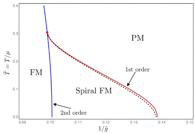
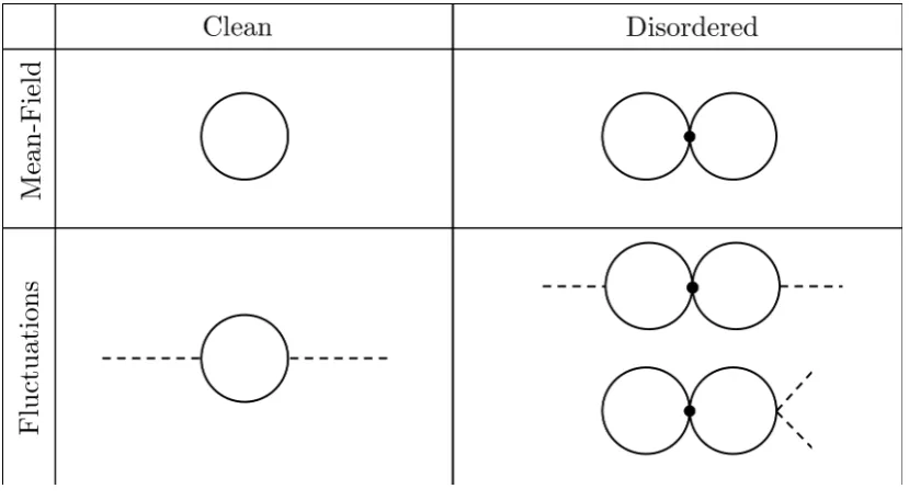
The fermionic order-by-disorder mechanism [83] is one of the proposed ways to extend and repair the conventional Hertz-Millis theory by including low-energy particle-hole fluctuations which couple to the order parameter and result in additional non-analytic corrections to the free energy. These fluctuation corrections reproduce the experimentally seen first-order behaviour in the vicinity of quantum critical points as well as the stabilisation of incommensurately ordered magnetic phases.

The name ‘order-by-disorder’ refers to the competition between internal energy and entropy rather than to any impurities or randomness. Previous work dealt purely with clean systems. My contribution to this mechanism, motivated by Ref. [84], was to consider the addition of quenched charge disorder into the system. We found that new fluctuation-corrections arise due to the presence of disorder in the system and these change the nature of the incommensurate phase from a long-range-ordered spiral ferromagnet to a new fluctuation-induced short-range ordered helical glass phase unlike anything predicted before in the literature.

2.2 Stoner Mean-Field Theory

The conventional mean-field theory of itinerant ferromagnetism in a fermionic Hubbard model is known as Stoner ferromagnetism [85, 86]. Before going on to more sophisticated extensions, we’ll take a look at the mean-field description of the paramagnet to ferromagnet transition.

We start from the fermionic Hubbard Hamiltonian:

ˆ

H= X

k, =±

["(k) µ] ˆnk, +g

X

i

ˆ

ni,+nˆi, , (2.1)

where ˆn is the fermionic number operator, =_±refers to the spin index, "(k) = k2_{/2 is the free-electron dispersion,} _g _{is the usual Hubbard contact interaction}