Exploiting NMR Spectroscopy for the Study of Disorder in Solids
Robert F. Moran, Daniel M. Dawson and Sharon E. Ashbrook*
School of Chemistry, EaStCHEM and St Andrews Centre of Magnetic Resonance, University of St Andrews, North Haugh, St Andrews KY16 9ST, UK
*Author to whom correspondence should be addressed.
E-mail: [email protected]
Abstract
Although the solid state is typically characterised by inherent periodicity, many
interesting physical and chemical properties of solids arise from a variation in this, i.e., changes in the nature of the atom occupying a particular site in a crystal structure or
variation in the position of an atom (or group of atoms) in different parts of a structure, or
variation as a function of time. This lack of long-range order poses significant challenges,
not just for the characterisation of the structure of disordered materials, but also simply for
its description. The sensitivity of nuclear magnetic resonance (NMR) spectroscopy to the
local, atomic-scale environment, without the requirement for long-range order, makes it a
powerful tool for the study of disorder in the solid state. Information on the number and
type(s) of coordinating atoms or through-space and through-bond connectivity between
atomic species enables the construction of a detailed picture of the structure. After a brief
description of the background theory of NMR spectroscopy, and the experimental
methods employed, we will describe the effects of disorder on NMR spectra and the use of
calculations to help interpret experimental measurements. We will then review a range of
applications to different types of disordered materials, including oxides and ceramics,
minerals, porous materials, biomaterials, energy materials, pharmaceuticals, polymers and
glasses. We will discuss the most successful approaches for studying different materials,
and illustrate the type of information available and the structural insight gained.
Keywords
1. Introduction
Although the solid state is typically characterised by long-range order or periodicity,
many of the more interesting physical and chemical properties of solids arise from a
variation in this, i.e., from some form of disorder. Variations in composition or atomic positions can lead to significant changes in the properties of a material, e.g., increasing ionic or electrical conductivity, improving chemical, mechanical or thermal stability or
enabling ferroelectric or magnetic behaviour. The sensitivity of many properties to even
very small changes in composition or structure, enables a system to be “tuned” to obtain
the desired behaviour under specific conditions, providing a variety of applications of
disordered materials in the energy arena, in the electronics industry, for construction, as
catalysts, for waste storage and in the pharmaceutical industry.
The characterisation of solid-state structure is typically dominated by methods
based on Bragg diffraction. For ideal solids (such as that shown schematically in Figure
1a), the long-range order in both atomic positions and site occupancies enables diffraction
to produce a complete and accurate structure solution from single-crystal measurements
or, in some cases, from powder data. However, any variation in periodicity hinders this
procedure, with diffraction then able only to provide information on the “average”
structure. For example, Figure 1b shows a schematic crystal structure where the
periodicity of the atomic positions is retained, but the atom occupying one of the
crystallographic sites varies. In this case of compositional disorder, it is typical for a
structure refinement to determine the atomic coordinates precisely, but to define a site as
having a fractional occupancy, e.g., B0.5C0.5 for the second atom in Figure 1b. While this
nomenclature indicates that two atom types are found at a particular site in the structure,
it does not provide any information on how the two might be distributed over these sites –
whether this distribution is random, or whether any clustering or preferred avoidance
occurs. In other cases, as shown schematically in Figure 1c, the position of atoms or groups
of atoms (e.g., OH–
, H2O, F –
vacancy. For example, in Figure 1c the A sites have a fractional occupancy of 0.75
(indicating each is vacant in 25% of cases). However, some caution is needed here as, more
generally, it is not clear from a fractional occupancy whether a site is occupied in 25% of
the material (as in Figure 1c) or for 25% of the time, i.e., a dynamic rather than a static disorder. Significant positional variation (be it static or dynamic) may result in atoms or
molecules not being located at all in the structure solution. This is often the case for water
or solvent molecules in pharmaceuticals, minerals or microporous materials. In addition to
fractional occupancies, it may be that variations in local geometry, i.e., bond distances and bond angles are present in a material. As this becomes more significant, the definition of a
“crystal structure” becomes less clear, posing significant challenges for diffraction-based
approaches. This is the case for amorphous materials, such as glasses, as shown in Figure
1d, where specific “sites” can no longer be defined and, while the local geometry around a
type of atom is often very similar, the long-range structure is now very different.
As the level and nature of disorder increases, Bragg diffraction (and perhaps even
the idea of “the crystal structure” itself) becomes less useful. In order to fully describe the
structure of a disordered solid it is necessary to consider not only any periodic aspects of
the structure that are retained, but also the changes in local geometry, e.g., the number and type of coordinating atoms, the nature of species on the next nearest neighbour (NNN)
sites and the variation in the bonding geometry. In this respect, nuclear magnetic
resonance (NMR) spectroscopy provides an ideal (and complementary) tool, with the
chemical shift a very sensitive probe of small changes in the local environment, and
couplings between nuclear spins (both through bond and through space) able to provide
information on covalent bonding and spatial proximities.[1] This has resulted in NMR
spectroscopy becoming one of the most widely-used analytical tools in the chemical
sciences, with widespread applications in many fields. However, unlike their
solution-state counterparts, NMR spectra of solids often contain broad and featureless lineshapes
as a result of the anisotropic (i.e., orientation-dependent) nature of the interactions that affect the nuclear spins – interactions that are averaged in solution by the rapid tumbling
improving resolution, some involving physical manipulation of the sample, such as
magic-angle spinning (MAS),[5] others just a manipulation of the nuclear spins, such as
decoupling. The spectra of nuclei with higher spin quantum number (i.e., I > 1/2) are also affected by an interaction with the electric field gradient (the quadrupolar interaction),
resulting in a broadening that cannot be removed by MAS and more complex techniques
are required to obtain high-resolution spectra.[1,6-8]
Even when high-resolution approaches are used, solid-state NMR spectra may still
contain complicated or overlapped spectral lineshapes, particularly as the structural
complexity and/or level of disorder in a material increases. This hinders resolution, and it
can be difficult both to assign the spectral resonances and to extract accurately the
structural information available. In general, NMR spectra of solids are more complicated
than those from solution-state experiments as the crystal packing in a solid produces not
only chemically- but also crystallographically-distinct species. Although, for molecular
solids, some insight can be gained through comparison to solution-state NMR spectra, this
does not help assign resonances from sites rendered inequivalent only by the packing,
which have very similar chemical environments and, therefore, very similar NMR
parameters. For many extended inorganic solids there is no molecular solution-state
counterpart to provide insight, and typically a range of less commonly-studied nuclear
species are investigated (many of which have inherently low natural abundance or low
sensitivity) and with, often, relatively little information in the literature to aid spectral
interpretation. Additional information can be obtained by measuring the magnitude of the
NMR parameters (both isotropic and anisotropic) although, in the latter case, this can
require recoupling (i.e., a selective reintroduction of interactions removed by techniques such as MAS), or by the use of experiments that transfer magnetisation between nuclear
spins, providing information on through-bond and through-space interactions.
The challenge in assigning and interpreting solid-state NMR spectra (and directly
producing a similar sort of structural picture to that available from diffraction) has
predict NMR parameters for a structure or structural model.[9-11] Although well
established for molecular systems, with a variety of codes available, such approaches have
only become widespread in the solid-state NMR community since the advent of
approaches able to calculate NMR parameters for periodic systems, i.e., exploiting the inherent transitional symmetry of the solid state.[12] For ordered crystalline solids,
calculations can be used to assign well-defined spectral resonances, to confirm unexpected
NMR parameters, or to predict the magnitude of parameters that are difficult to extract
experimentally (including anisotropic interactions or tensor orientations), in many cases
guiding experimental measurements or analytical fitting procedures. Calculations often
play a vital role in the emerging field of NMR crystallography (the use of NMR
spectroscopy, often in combination with diffraction experiments, to solve or refine
structures).[13,14] For disordered materials, the computational challenge is much greater,
with the deviation from periodicity often requiring a large number of different
calculations to be performed and/or larger supercells employed. However, the ability to
predict NMR parameters for species with varying local and long-range environments
provides insight into the interpretation of the complex spectral lineshapes and important
information about the local structural environments present.
In this review, we will discuss the use of solid-state NMR spectroscopy to
investigate the structure of disordered materials. After a brief description of the
background theory and the experimental methods employed, we will describe the effects
of disorder on NMR spectra and the use of calculations to help interpret experimental
measurements. We will then review a range of applications to different types of
disordered materials, including oxides and ceramics, minerals, porous materials,
biomaterials, energy materials, pharmaceuticals, polymers and glasses. Clearly, this
cannot be a comprehensive review of each area, but we hope to discuss the most
important considerations and most successful approaches for different materials, and to
illustrate the type of information available and the insight gained by discussing some
selected case studies in more detail. For further information on each area, readers are
2. Basics of Solid-State NMR
2.1 Magnetisation and Pulses
NMR spectroscopy is concerned with the interaction of electromagnetic radiation with the
intrinsic magnetic moments of nuclei. The nuclear magnetism arises from the
quantum-mechanical nuclear spin, I, (where the bold typeface represents a vector quantity)
described by the quantum number, I. As I arises from the combined spins of the protons
and neutrons (both of which have I = 1/2), I may take any integer or half-integer value.
The nuclear magnetic moment, µ, is given by
µ = γ I , 1
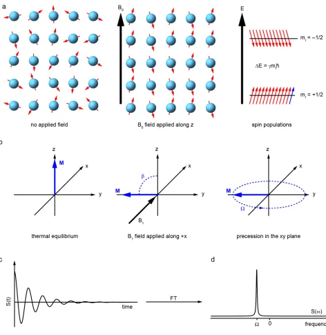
where γ is the gyromagnetic ratio, characteristic of a given nuclide. As shown in Figure 2a,
in an external magnetic field, B0, (magnitude B0), the magnetic moments are quantised
along the field direction (by definition the z axis) in units of ħ, with
µz = γ mIħ , 2
where mI is the magnetic quantum number, which can take any integer or half-integer
value between –I and +I. The energy of each spin state (the Zeeman energy) is given by –
µzB0 and the energy difference, ΔE, between two states is, therefore,
ΔE = ΔmIγ ħ B0 . 3
As only single-quantum transitions (ΔmI = ±1) are allowed by the NMR selection rules, all
observable transitions occur with ΔE = γ ħ B0, corresponding to a frequency (termed the
Larmor frequency) of ω0 = –γ B0 in rad s –1
or ν0 = ω0/2π in Hz. Typical B0 fields used range
from 4 to 24 T, giving rise to Larmor frequencies corresponding to the radiofrequency (rf)
region of the spectrum, on the order of ~5-1000 MHz.
In a macroscopic ensemble of spins, the Zeeman states are populated according to a
Boltzmann distribution, with
NmI+1 Nm
I
where N is the population of the corresponding mI state, kB is Boltzmann’s constant and T
is the absolute temperature. For I = 1/2 nuclei, the population difference between the two
spin states (mI = ±1/2) gives rise to a bulk magnetisation, M, which can be considered as
the observable in an NMR experiment, as shown in Figure 2. As the population difference
is typically on the order of a few spins in 105
to 107
, M is very small and NMR spectroscopy is inherently insensitive, leading to considerable interest in approaches for
improving sensitivity in many aspects of the technique. At thermal equilibrium, M is aligned along z and precesses about this axis with frequency, ω0. The magnetisation can be
manipulated by the application of short bursts of rf irradiation, or “pulses” with
frequency, ωrf≈ω0. The effect of a pulse is most easily considered in the rotating frame – a
coordinate system in which the z axis remains aligned with the laboratory z axis (defined
by B0) and the xy plane rotates about the z axis at ωrf. In this rotating frame, and as shown
in Figure 2b, the pulse appears as a static field, B1, (magnitude B1), in the xy plane and M
now precesses about z at an offset frequency, Ω, where
Ω = ω0 – ωrf , 5
which then implies an effective field along z of
Beff = Ω/γ . 6
When a pulse is applied “on resonance” ωrf = ω0, Beff = 0 and M nutates about B1 at a
frequency
ω1 = – γ B1 . 7
Over the duration of the pulse, τp, M will nutate through a “flip angle”,
β = ω1τp . 8
Once the B1 field is removed, M will again precess about z at frequency Ω, but now has a
component in the xy plane. Over time, M will return to equilibrium through spin-lattice or longitudinal relaxation, described by the time constant, T1, typically on the order of
seconds to hours for solids. In addition, the magnetisation in the xy plane will “dephase”
through spin-spin or transverse relaxation processes, described by the time constant, T2.
For solids, the apparent transverse relaxation (often termed T2*)[15] is generally much
The precession of M in the xy plane is recorded as the complex time-domain signal, S(t), or free induction decay (FID), as shown in Figure 2c, where the acquisition of both
real and imaginary components (or “quadrature detection”) by two detector coils allows
the sense of precession to be determined. Assuming T1 ≫ T2, the FID can be written as
S t
( )
= ei Ω t e–t T2 , 9and Fourier transform yields the frequency-domain spectrum, S(ω), the real component of
which is an absorptive Lorentzian function centred at Ω and with a full width at half
height of 1/πT2, as shown in Figure 2. As stated above, NMR spectroscopy is inherently
insensitive and, consequently, the signal in the FID is generally accompanied by a large
amount of electronic noise. This can be overcome by “signal averaging”, where N FIDs are
coadded with a “recycle interval” between successive acquisitions to allow magnetisation
to return to equilibrium. As the signal increases linearly with N, whereas the random
noise accumulates with √N, the signal-to-noise ratio (SNR) increases as √N. The return of
the z component of M, Mz, to thermal equilibrium is given by Mz
( )
t = M0 1 – e–t T1
(
)
, 10meaning that equilibrium (Mz(t) > 0.99 M0) is only achieved at t ≈ 5 T1. As a consequence,
NMR experiments can be very time consuming for nuclei with low sensitivity or slow
longitudinal relaxation.
2.2 Internal Interactions
Much of the practical value of NMR spectroscopy comes from the fact that nuclear
magnetic moments interact not just with the external magnetic field, but also with their
local surroundings (i.e., other nuclear spins, electrons and electric field gradients).[2-4]
These interactions alter the resonant frequency of the nucleus (generally by a few Hz to
tens of kHz, compared to the 10-800 MHz Larmor frequency), making NMR spectroscopy
an exquisitely sensitive probe of not just which nuclei are present in the material, but where
exactly they are with respect to their surroundings. One of these interactions, the chemical
shielding, arises from the motion of electrons in orbitals near the nucleus.[16] This motion
B = B0 – B’ = B0 (1 – σ) , 11
where σ is the field-independent shielding constant. It is practically challenging to
measure the absolute value of σ and, instead, the chemical shift, δ, of an observed
frequency, ωobs, is generally quoted relative to a reference, ωref, with δ = 106×
(ωobs – ωref) / ωref , 12
where the factor of 106
accounts for the fact that δ is normally quoted as parts per million
(ppm). As the sign of δ is opposite to that of σ, δ describes a deshielding scale. In solution, rapid molecular tumbling means that an average, or isotropic, chemical shift, δiso, is
observed, whereas such motion is absent for (most) solids and δ is anisotropic, described
by a second-rank tensor, δ. In the principal axis system (PAS), δPAS
is diagonal, with
principal components δ11, δ22 and δ33, with |δ11 – δiso| ≥ |δ33 – δiso| ≥ |δ22 – δiso| in the
Haeberlen notation[17] (other notations are also commonly used – see Ref. [17] for details).
The isotropic shift is given by
δiso = Tr {δ} = (δ11+δ22+δ33) / 3 , 13
the anisotropy of the tensor, ΔCS, is defined as
ΔCS = δ33–δiso , 14
and the asymmetry by
ηCS = (δ22–δ11) / ΔCS , 15
such that 0 ≤ ηCS ≤ 1. The observed chemical shift is given by δ = δiso + (ΔCS/2) [(3 cos
2θ
– 1) + ηCS (sin 2θ
cos2φ)] , 16
where the polar angles, θ and φ, describe the orientation of δ relative to the laboratory
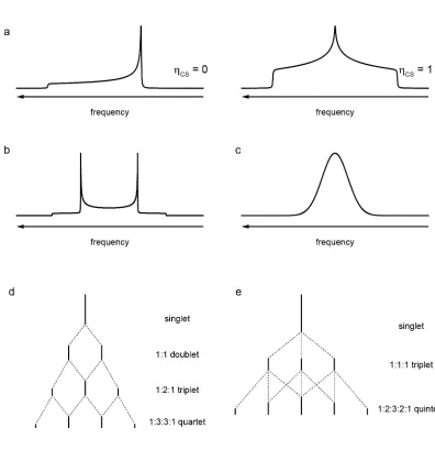
frame. This chemical shift anisotropy (CSA) gives an orientation-dependent resonance for
a single crystallite, and a characteristic powder-pattern lineshape, whose width depends
on ΔCS and whose shape depends on ηCS, as shown in Figure 3a. In an alternative
formalism,[17] the anisotropy can also be described in terms of the span
Ω = δ11–δ33 , 17
a measure of the magnitude, and the skew
κ = 3(δ22 – δiso)/Ω , 18
Nuclear spins can also interact with each other, either via the through-space dipolar coupling, or the electron-mediated J (or “scalar”) coupling.[18] In the PAS, the dipolar
interaction tensor, DPAS
, is traceless (i.e., there is no “isotropic dipolar shift”) and axially symmetric (ηD = 0). The dipolar coupling between two spins, I and S, separated by a
distance, rIS, gives rise to a splitting of
(
)
= 0 I S 2
D 3 IS
IS
h 1
3 cos – 1
4 r 2
µ γ γ
ω θ
π , 19
where θIS is the angle between the internuclear vector and B0. For a given I/S spin pair, the
only variable in Equation 19 is rIS, making the dipolar coupling, in principle, a very
sensitive measure of internuclear distances in solids. For isolated (I = S = 1/2) spin pairs in
a powdered sample, the dipolar coupling gives rise to a “Pake doublet”, as shown in
Figure 3b. Such cases are rare and in reality a nucleus will generally experience multiple
dipolar couplings of different magnitudes, leading to a more Gaussian-like lineshape,
shown in Figure 3c.
The scalar coupling occurs as nuclear spins can polarise nearby electrons (typically
in bonds), which then transfer this polarisation to other nearby nuclei. In solution, the
scalar coupling leads to an isotropic splitting characteristic of the number and spin
quantum number of the coupled nuclei, as shown in Figures 3d and 3e. The magnitude of
the scalar coupling constant, J, typically decreases with the number of bonds through
which the coupling occurs, in principle allowing the scalar coupling interaction to be used
to probe through-bond connectivity. However, as J rarely exceeds a few hundred Hz, the
effects of the scalar coupling are often masked by other internal interactions in solids, and
coupling patterns are rarely resolved. While J is technically a tensor quantity, giving rise to
an anisotropic broadening as well as an isotropic splitting, only the isotropic splitting is
generally considered as the anisotropy is sufficiently small as to be negligible under most
common experimental conditions (as discussed below).
In addition to the interactions discussed above, nuclei with I > 1/2 possess a
(EFG), described by the tensor, V.[6-8,19] In its PAS, VPAS
is diagonal and traceless, with
components |Vzz| ≥ |Vyy| ≥ |Vxx|. The interaction of eQ with V is described by its
magnitude, the quadrupolar coupling constant,
CQ = e Q Vzz/h , 20
and asymmetry,
ηQ = (Vxx – Vyy) / Vzz , 21
with 0 ≤ηQ≤ 1. The quadrupolar product, PQ, can also be defined as
PQ = CQ (1 + (ηQ 2
/3))1/2
, 22
giving CQ≤ PQ ≤ 1.155 CQ. When the EFG at the nucleus is zero, all single-quantum (ΔmI =
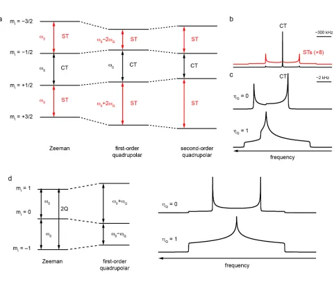
±1) transitions occur at ω0. The effect of a small EFG can be considered as a first-order
perturbation of the energy levels (shown for the case of I = 3/2 in Figure 4a), with
ωQ = (ωQ PAS
/2) (3 cos2β
– 1 + ηQ sin 2β
cos 2γ) , 23
where β and γ are two of the Euler angles relating the PAS to the lab frame and (in rad s–1
)
ωQ PAS
= 3π CQ/2I (2I – 1) . 24
For half-integer spins, the first-order perturbation leads to a differentiation between the
central transition (CT, mI = +1 ↔ mI = –1) and the other single-quantum “satellite”
transitions (STs) and, for a powdered sample, the CT occurs as a sharp line at ω0 (i.e.,
unaffected by the quadrupolar interaction), whereas the STs are broadened into Pake
doublets, as shown in Figure 4b. Although they cannot be observed directly, it should be
noted that the symmetrical multiple-quantum (MQ) transitions (ΔmI = +n ↔ΔmI = –n) are
also unaffected by the first-order perturbation. The influence of a larger EFG can be
considered as a second-order perturbation of the Zeeman energy levels, as discussed
further in Refs. [6-8, 19]. The second-order perturbation affects all transitions, with the STs
broadened typically over several MHz and the CT shifted from ω0 by an isotropic
quadrupolar shift, δQ, and broadened, typically by 1-10 kHz. In such cases, only the CT is
observed, with its width proportional to CQ and a characteristic shape dependent on ηQ, as
shown in Figure 4c. The magnitude of the second-order quadrupolar interaction is
proportional to (ωQ 2
/ω0), and so decreases with increasing B0 field. For nuclei with integer
spin quantum number, there is no CT and all single-quantum transitions are
4d for I = 1. However, the symmetrical multiple-quantum transitions (ΔmI = +n ↔ΔmI = –
n) are unaffected to first order.
In addition to all of the interactions described above, when unpaired electrons are
present, these may also affect the isotropic shifts and anisotropic broadening of
resonances.[20,21] As electrons have spin I = 1/2 and a gyromagnetic ratio ~660 times
greater than 1
H, through-bond and through-space interactions with unpaired electrons can
be large and long range. The through-bond interaction is mechanistically analogous to the
scalar coupling, but termed the hyperfine/transferred hyperfine interaction, with a
coupling constant, A/ħ, usually on the order of MHz. However, as the electronic
relaxation is many orders of magnitude more rapid than nuclear relaxation, the nuclei
experience only a thermally-averaged electronic spin state (rather than discrete α and β
spins), leading to a temperature-dependent isotropic shift rather than a splitting. The
through-space pseudocontact interaction is mechanistically similar to the internuclear
dipolar interaction, except that the electron spins are again thermally averaged, leading to
a small isotropic shift in addition to the anisotropic broadening. Where present, the
hyperfine coupling tends to dominate (with shifts of many hundreds or thousands of ppm
possible) but both interactions are generally described by a single “paramagnetic shift
anisotropy” (PSA) tensor, analogous to the CSA.[21] The rapid electronic relaxation can
also induce very rapid nuclear T1 and T2 relaxation, often several orders of magnitude
faster than in analogous diamagnetic materials. However, the precise effects of the
unpaired electrons will depend strongly on the types of bonding present and the
distribution of the paramagnetic centres within a material.
From the above discussion, it can be seen that an NMR spectrum of a material will
contain a wealth of information: the number of resonances corresponds to the number of
magnetically-distinct species (arising from chemical or crystallographic inequivalence),
peak integrals should correspond to site populations, the anisotropic broadening contains
information on point symmetry, the dipolar coupling can (in principle) be used to measure
network present.[2-4] However, in general, all of this information is present
simultaneously and, in most cases, the isotropic part of an interaction is much smaller than
the anisotropic part. Therefore, when multiple resonances are present, their width tends to
exceed their separation, leading to broadened and overlapped lineshapes that can often be
very challenging to interpret, even for perfectly crystalline and ordered materials.
3. Experimental Methodology
From Section 2, it is clear that NMR spectra of solids suffer from two inherent problems –
low resolution and sensitivity – and many experimental approaches have been developed
to overcome these. The resolution obtained from solution-state NMR spectroscopy is
much greater than for solids, as the rapid isotropic molecular tumbling present leads to an
effective averaging of the anisotropic interactions to their isotropic values. Such motion is
not generally present in solids, but can be mimicked using the technique of magic angle
spinning (MAS),[5] shown schematically in Figure 5a. In a MAS experiment, the sample is
packed into a holder, or rotor, oriented at the “magic” angle of θm = 54.736° to the z axis,
and then rapidly rotated. If the rotation is sufficiently rapid (rotation rates up to at up to
~111 kHz are available using commercial hardware), MAS achieves the same average
orientation (θ = 54.736°) for every crystallite, such that terms with an orientation
dependence of (1/2)(3cos2θ
– 1), i.e., the chemical shift, dipolar and J couplings and the first-order quadrupolar interaction, are averaged to their isotropic values (0 for the dipolar
and quadrupolar couplings, δiso for the chemical shift and J for the J coupling), as seen in
Figure 5b.[2-4] If the MAS rate, ωR, is “slow” compared to the magnitude of the interaction
to be removed, the powder-pattern lineshape is broken into a series of spinning sidebands
(as seen in Figure 5b), separated by integer multiples of ωR, with intensities related to the
static lineshape.[22] MAS is routinely used to enhance resolution, and has the added
advantage that the spectral intensity is focused into narrow isotropic resonances (and
For quadrupolar nuclei, MAS is capable (in principle) of removing the first-order
anisotropic quadrupolar broadening, although the magnitude of this interaction typically
means that the ST are observed as a series of sharp spinning sidebands spanning
hundreds of kHz.[2,3,6] However, MAS while narrowing the lineshape is unable to
completely remove the second-order anisotropic quadrupolar broadening of the CT,
owing to its more complex angular dependence. It is not possible to remove the
second-order quadrupolar broadening by spinning around a single angle, but it is possible to
achieve this by spinning at two angles simultaneously, as performed in the double
rotation (DOR) approach.[2,23] In DOR, a sample is rotated at an angle of 30.56° in a rotor
that is held within a second rotor, inclined at 54.74°, using a specialist probe. However, the
technical challenges of achieving stable spinning at two angles, and the diameter of the
large outer rotor restrict the maximum rotation rate of the inner rotor to ~2 kHz and DOR
spectra are often cluttered by spinning sidebands. Alternative methods, combining
multiple-pulse sequences and standard probe hardware to achieve high resolution, are
discussed below.
Heteronuclear spin-spin interactions (i.e., dipolar and scalar couplings) can be
removed by decoupling,[2,3,24] the simplest form of which involves observing the FID for
one spin, I, while continuously irradiating the coupled spin, S. Such continuous-wave
(CW) decoupling induces continuous transitions of the S spins, such that the average
coupling is zero. However, when the MAS rate is rapid, or the S spins experience large
anisotropic interactions (e.g., CSA or quadrupolar), more efficient decoupling sequences may be required, and many of these have been developed (with a greater or lesser degree
of transferability between different systems). Decoupling of homonuclear
couplings[2,3,25] is particularly challenging, as it involves the simultaneous irradiation
and observation of the same spin. This is usually achieved by a complex “windowed”
sequence, in which multiple pulses are applied to periodically refocus the homonuclear
interactions to zero, with a data point recorded each time this occurs. Combining this with
many of the timings in the sequence to be synchronised with the sample rotation,
imposing stringent requirements for experimental implementation.
In many cases, once a high-resolution spectrum has been achieved, it is desirable to
reintroduce an interaction in a selective and controlled manner, such that its effect can be
observed in the spectrum or it can be measured indirectly. A range of experiments have
been developed to reintroduce the dipolar interaction (for the measurement of direct
measurement of interatomic distances) and the CSA.[2,3,27-30] Information can also be
obtained by transferring magnetisation between nuclear spins, typically measured using
two-dimensional spectra.[31,32] A general two-dimensional experiment comprises four
parts: preparation, evolution, mixing and detection. Preparation involves excitation of the
first spin (or spins), via a pulse or series of pulses, with the magnetisation then allowed to evolve in a subsequent period of time (or time intervals and pulses), termed t1. In the
mixing stage, magnetisation is transferred between either heteronuclear or homonuclear
spins. Finally, in the detection period, t2, the signal (i.e., FID) is recorded. The intensity of
the signal recorded in t2 is modulated by any evolution of the magnetisation in t1 and,
therefore, by recording a series of one-dimensional FIDs for systematically increasing
values of t1, it is possible to construct a two-dimensional dataset with “direct” (t2) and
“indirect” (t1) dimensions. For nuclei with I = 1/2, two-dimensional experiments are most
commonly used to transfer magnetisation between nuclei (generally termed “correlation
experiments”) to determine the spatial (if the transfer is via the dipolar coupling) or covalent (if the transfer is via the scalar coupling) connectivity of a material. Two-dimensional experiments can also be used to reintroduce interactions such as the CSA or
scalar coupling in the indirect dimension (see above), allowing their accurate
measurement where this is not possible from the MAS spectrum.[27, 29, 33]
For quadrupolar nuclei, the most popular two-dimensional experiment by far is the
multiple-quantum (MQ) MAS experiment,[6,34] in which (after appropriate processing)
the indirect dimension contains an isotropic spectrum with no contribution from the first-
the direct dimension contains MAS lineshapes from which the quadrupolar interaction
parameters can be determined, as shown in Figure 5c. The experiment does not involve
the transfer of magnetisation between spins, as discussed above, but rather the correlation
of different transitions within the spin system, with the aim of removing completely the
second-order quadrupolar interaction. However, MQMAS suffers from poor sensitivity,
owing to the use of a formally “forbidden” multiple-quantum transition. While much
effort has been devoted to developing pulse schemes[35-37] to improve the sensitivity of
the experiment, the related satellite transition (ST) MAS experiment[6,38,39] offers much
higher inherent sensitivity (owing to the use of only allowed single-quantum transitions
throughout the experiment), albeit at the cost of a more exacting experimental setup in
terms of MAS stability and the precision of the magic angle setting. Both experiments are,
however, typically preferred to the one-dimensional DOR technique discussed above, as
there is no need for specialist hardware. The vast majority of the two-dimensional
magnetisation transfer experiments used for I = 1/2 nuclei can also be applied to
quadrupolar nuclei.[2,6,27] This will result in a broadened lineshape for the quadrupolar
nucleus unless an initial MQ filtration step is applied in order to achieve high resolution.
In addition to issues with resolution, another major challenge facing solid-state
NMR experiments is the inherently poor sensitivity. This arises not only from the low
Boltzmann population differences at or near room temperature, but also from either the
dilution of NMR-active isotopes (e.g., the only NMR-active isotopes of the two ubiquitous elements, C and O, 13
C and 17
O have natural abundances of just 1.07% and 0.037%,
respectively). It is possible to enhance the spin polarisation either by transfer from a
nearby nucleus with higher polarisation (and, typically, higher abundance) such as 1
H or
19
F using the cross polarisation (CP) experiment.[40,41] In a CP experiment, an initial 90°
pulse creates transverse magnetisation on the I spins, and this is transferred to the S spins
(through the dipolar coupling between them) by simultaneous irradiation of both nuclei
during a “spin lock” period. The rf field strength of the spin lock pulses must be
“matched” such that ω1I = ω 1S (± nωR in the case of MAS) in order to achieve efficient
the time constant TIS (dependent on the magnitude of the dipolar coupling) and decays by
a process described by the time constant T1ρ. When T1ρ ≫ TIS, it is possible to achieve a
theoretical polarisation enhancement of ~γS/γI (i.e., a factor of ~4 for 1
H and 13
C). As
polarisation is transferred via the dipolar interaction, CP is a non-quantitiative technique, with polarisation building up more rapidly for species such as CH3 than for, e.g., CO2
–
.
This non-quantitative nature of CP can be of use when assigning chemically-distinct
species with similar chemical shifts. CP often provides no signal enhancement for
quadrupolar nuclei, as it is difficult to achieve a transfer match for all crystallites present.
However, the experiment can still be used for signal editing and spectral assignment, e.g., to distinguish between SiOSi and SiOH resonances. Another approach to improving sensitivity is the use of a Carr-Purcell-Meiboom-Gill (CPMG) echo train.[42,43] The
application of a series of 180° pulses during acquisition results in an FID that consists of
multiple echoes, and subsequent Fourier transformation yields a spectrum consisting of a
series of “spikelets”, with intensities that reflect the lineshape, increasing the peak-height
signal. The use of CPMG under MAS requires that the pulses are applied synchronously
with the sample rotation.
The signal enhancement factor that is practically achievable when using other
nuclei as the source of polarisation is generally of the order of a factor of 2-10 (although
the typically more rapid relaxation of the I spins leads to a sensitivity enhancement per
unit time that can be ca. two orders of magnitude). An alternative source of polarisation would be electrons, which have a much greater spin polarisation. The technique of
dynamic nuclear polarisation (DNP) introduces unpaired electrons into a material in the
form of (typically) nitroxide-based radicals.[44,45] At the magnetic fields used for NMR
experiments, the electrons have a resonance frequency in the microwave region, and
irradiation of the sample with microwaves followed by spin diffusion leads to a
highly-polarised 1
H population. From here, the magnetisation can be transferred (e.g., by CP) to the nucleus of interest, leading to a sensitivity enhancement factor of, in principle, up to
γe/γH ≈ 660, but, in practice, of 10-100. Although an extremely promising technique for
suitable microwaves) and experiments to be performed at low (e.g., 100 K) temperatures, posing a technical challenge and limiting the possible rotation rates. DNP is also surface
sensitive and currently requires a sample to contain sufficient 1
H in close proximity to the
species of interest. Applications to proteins, organic systems, polymers and catalyst
surfaces have been demonstrated,[44,45] but it is yet to be seen how routine this approach
will become in the future for a wide range of systems.
In some cases, the resonance of interest is so broad that MAS is not a practical
option (e.g., in paramagnetic samples or cases of very large values of Ω or CQ) and it is
more suitable to record the static lineshape.[6,46] Such “wideline” spectra are often
recorded in a frequency-stepped fashion (i.e., in a series of sub spectra) in order to ensure uniform excitation at all frequencies, thereby avoiding any distortion of the lineshape.
However, this can be time-consuming and practically challenging, and various broadband
excitation pulses have been successfully applied (generally in conjunction with CPMG
echo trains) to reduce the number of frequency steps required.
4. The Effects of Disorder on NMR Spectra
Any variation in the local environment of a nucleus will result in changes to the NMR
parameters, i.e., in the isotropic and anisotropic shielding, the couplings between spins and the quadrupolar coupling. Unless dynamics are present (see below) the NMR
spectrum of a disordered material can be seen as the sum of signals from every individual
environment present. Hence, the appearance of the spectrum will depend on the type and
extent of disorder present, and the magnitude of the changes in the NMR parameters.
If polymorphic disorder is present (i.e., the atoms and/or molecules adopt completely different spatial arrangements within a solid), the NMR spectrum may be
significantly different in each case. This was shown in work on 17
O NMR spectra of four
polymorphs of MgSiO3,[47] where each material had different numbers of distinct O
the conditions required to synthesise each polymorph (i.e., the required temperature and pressure) are very different, and it is not likely they would be produced in the same
sample. However, for many molecular and inorganic solids, this is not the case and there
are a number of polymorphs with similar energies at room temperature and pressure,
which can appear together in the same bulk sample. This is particularly true for small
organic molecules and pharmaceuticals, and can pose a challenge for understanding a
bulk material, if the structure solution is carried out by single-crystal diffraction (which,
by definition, studies only a single polymorph per measurement). A similar problem can
also be found for some inorganic materials, as shown in recent work on a range of niobate
perovskites.[48-50] Peel et al.[50] showed that not only did samples of LixNa1–xNbO3 (0.08 ≤
x ≤ 0.20) contain mixtures of a polar orthorhombic phase (P21ma) and a rhombohedral
phase (R3c), the relative fractions of the two phases were shown to be critically# dependent on synthetic conditions. Furthermore, the orthorhombic phase transformed slowly to the
rhombohedral phase on standing in air at ambient temperature, a process that could be
followed using 23
Na MQMAS NMR spectroscopy.[50]
If the variation in the local environment for an atom in a disordered material is
significant (e.g., a change in coordination number), then this can produce a significant difference in chemical shift, and the appearance of separate resonances in the NMR
spectrum. Less significant (or more remote) changes, in environment produce a smaller
variation in the chemical shift, and the appearance of shoulders or splittings on the
spectral lineshapes. When changes are much smaller (e.g., a variation in bond distances or angles), or are much more remote, the chemical shift change will be very small and
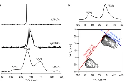
typically leads to a spectral broadening. These effects can be seen on the 89
Y NMR spectra
shown in Figure 6a. The 89
Y MAS spectrum of Y2Sn2O7 exhibits a single sharp resonance,
confirming one type of Y species is present, in a well-ordered solid, with the chemical shift
confirming that the Y has eight-fold coordination.[51] The substitution of Ti onto the NNN
sites in Y2SnTiO7 produces a number of shoulders and splittings of the lineshape, with the
chemical shift varying with the number and arrangement of surrounding atoms.[51] There
structural changes. The CPMG MAS spectrum of Y2Zr2O7 shows three very broad
lineshapes, with the shift ranges confirming the presence of 6-, 7- and 8-coordinate Y, as a
result of a disorder in the position of the oxygen vacancies in the structure.[52]
For systems where either only one geometrical parameter is varying, or where the
variation is much more significant than that in any other parameter, it may be possible to
relate the spectral broadening directly to the distribution of the geometrical parameters.
This has been attempted in glasses by a number of authors, with the width of 29
Si NMR
resonances being related directly to the distribution in the Si-O-Si bond angles.[53-55]
However, such analyses are often complicated both by the fact that even in simple systems
(e.g., SiO4 tetrahedra) more than one bond angle or distance needs to be considered.
Furthermore, in most practical cases more than one geometrical parameter will vary
simultaneously, complicating any quantitative spectral analysis. This was recently
investigated for aluminophosphate (AlPO) frameworks, where the 31
P chemical shift was
shown to depend not only on the average P-O-Al angle, as had been previously suggested,
but also on the average P-O bond distance.[56] When performing two-dimensional
experiments, the shape of the cross peaks observed, i.e., how the various contributions to each broad lineshape correlate with each other, can provide information on the spatial
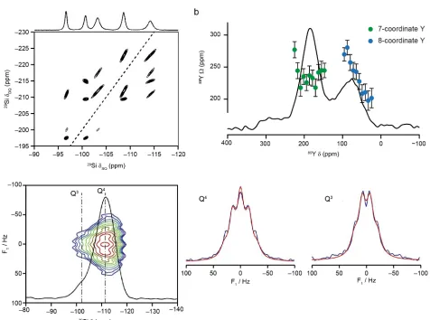
distribution of species in a sample. This can be seen in Figure 7a, where a 29
Si /29
Si
correlation spectrum of a surfactant-templated layered silicate is shown.[57] The elongated
nature of the cross peaks at higher temperature reveals the presence of correlated disorder,
with a Si species contributing to one part of one lineshape interacting (in this case through
covalent bonds) to Si species that have only one chemical shift within the second
resonance. More circular cross peaks, i.e., where all species that contribute to one lineshape interact with all that contribute to a second, would be observed if species were more
randomly distributed.
It is also possible to obtain information on the nature of the order/disorder of
surrounding species from the intensity of the spectral resonances. For example, if an atom
(X and Y), there are five possible local environments (X4, X3Y, X2Y2, XY3 and Y4).
Assuming these give rise to five resonances that can be resolved and accurately assigned,
the relative intensity of each can be directly related to the amount of that environment
present. Clearly, if clustering of X and Y is preferred, the intensity of the X4 and Y4
resonances will be greater than those from more mixed atomic distributions. Alternatively,
if there is some preference for ordering, the X2Y2 resonance might have higher intensity.
For a random distribution of the atoms on the surrounding sites, it is possible to predict
the expected intensity of the resonances expected using simple statistics. For the general
case, the probability of finding a particular environment, i.e., a atoms of species A, b of species B, c of species C, etc., on N surrounding sites is given by
P = (N!/a! b! c!...) (pA)a
(pB)b
(pC)c
… , 25
where pA, pB, etc., represent the probability of finding species A, B, etc., (which can be determined from the chemical formula), and a + b + c … has to equal N. For the specific
case described above, this can be simplified to
P = (N!/n! (N – n)!) (pX)n
(1 – pX))N–n
, 26
where pX represents the fraction of X and 1 – pX the fraction of Y in the sample. For
example, for pX = 0.6 (i.e., there is 60% X and 40% Y distributed on the four sites), the probability of finding X4, X3Y, X2Y2, XY3 and Y4 environments would be 13.0%, 34.5%,
34.5%, 15.5% and 2.5%, respectively. Therefore, if the relative spectral intensities are in
agreement with this analysis then it can be assumed that the atomic distribution is
random.
Although for spin I = 1/2 nuclei it is often changes to the isotropic chemical shift
that have the most significant effect upon the NMR spectrum, there are also changes to
other NMR parameters as the local environment varies in a disordered solid. Changes in
the isotropic shift result from a change in the principal components of the shielding tensor,
which can result in a concomitant change in the anisotropic parameters (Ω and κ).
Therefore, it is often seen that the anisotropy varies across a spectral lineshape, i.e., with a
change in δiso. This can be measured using amplified PASS experiments, where the use of
measured in the indirect dimension of a two-dimensional experiment. This is shown in
Figure 7b, where CSA measurements (specifically Ω = δ33 – δ 11), acquired using amplified
PASS experiments are shown overlaid on the 89
Y MAS NMR spectrum of Y2Zr2O7.[52]
Three 89
Y signals are seen (corresponding to YVI
, YVII
and YVIII
) owing to the disorder of the
oxygen vacancies on the anion lattice of this defect fluorite material. For YVIII
, Ω varies
across the broadened lineshape, decreasing with decreasing δiso. In contrast, there is little
change in Ω across the YVII
lineshape. The J coupling can also vary as the local
environment changes. For a disordered material, where the distribution of chemical shift
may well obscure any splittings resulting from J couplings, these can be measured in the
indirect dimension of a two-dimensional J-resolved spectrum. As shown in Figure 7c for a
29
Si spectrum of (29
Si enriched) SiO2, the changes in J can be correlated to those in the
chemical shift, resulting in a J coupling that varies at different positions within the spectral
lineshape.[58]
For nuclei with spin I > 1/2, variation in the local structure changes not only the
chemical shift, but also the magnitude and asymmetry of the quadrupolar interaction. As
the second-order quadrupolar interaction produces resonances that have a characteristic
shape (determined by ηQ) disorder produces not just a broadening of the line, but also a
change in its shape. This can be seen in the 27
Al MAS NMR spectrum of γ-Al2O3 shown in
Figure 6b, where the resonances display a characteristic “tail” to low frequency resulting
from the distribution of quadrupolar parameters.[6] The exact shape of the line is
determined by the magnitude (and the type) of the distributions in δiso, CQ and ηQ, and
whether these are correlated. It is difficult to extract this information from a single MAS
lineshape unless some assumptions about the distributions can be made. One approach to
simplify this problem is to assume a joint distribution in the quadrupolar parameters
using the Czjzek model (and its various extensions),[59-61] exploiting the fact that both CQ
and ηQ are related to the principal components of the EFG tensor. Thus, the distribution in
the quadrupolar parameters can be described by a single parameter. Lineshapes can then
be fitted assuming a Czjzek distribution of the EFG and, typically, a Gaussian distribution
considering the shape of the resonances in two-dimensional MQMAS spectra. As seen in
Figure 6b for γ-Al2O3, MQMAS lineshapes for disordered materials contain ridges that are
broadened along different gradients by distributions in chemical shifts and/or the
quadrupolar parameters. These axes are shown on the MQMAS spectrum in Figure 6b for
a spin I = 5/2 nucleus (note that, in the spectrum shown, an ordered material would
exhibit a ridge-like lineshape that lies parallel to the δ2 axis, as shown in Figure 5c).[62]
Using freely-available fitting programs,[63] it is possible to fit the two-dimensional
lineshapes (typically assuming a Czjzek distribution of the EFG and a Gaussian
distribution of the chemical shift) and extract the information on the magnitude of the
distribution of the NMR parameters present.
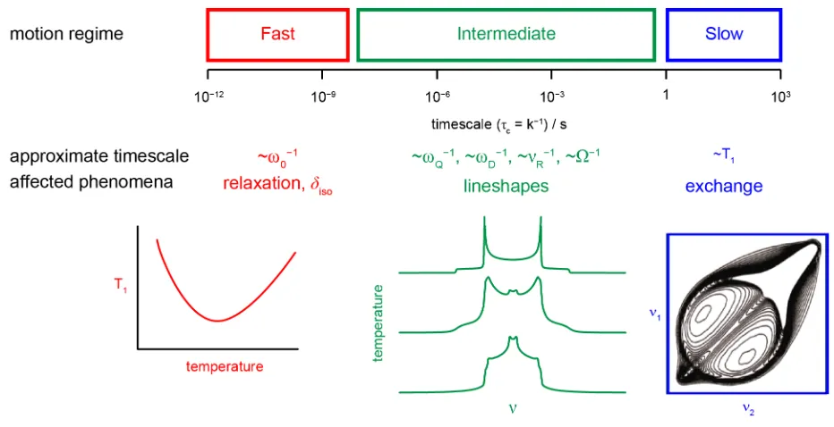
In many materials the positions of atoms or groups vary over time, leading to
temporal or dynamic disorder. It can be extremely challenging to distinguish this case
from that where atomic positions vary in different parts of a material (i.e., static positional disorder), with diffraction providing information simply on the average structure, and
refining sites as having a fractional occupancy. NMR spectroscopy, however, is sensitive
to motion on timescales spanning 15 orders of magnitude, as shown in Figure 8.[2,3] Very
fast motion leads to changes in the relaxation processes, with T1 relaxation affected by
dynamic processes with a correlation time τc ≈ 1/ν0. Slow motion can be measured using
two-dimensional exchange experiments, where cross peaks show the change in the NMR
parameters that result from the physical motion of an atom when a “mixing time” (usually
10–3
to 102
s) is introduced into the pulse sequence. Although resolution is higher in
MAS-based experiments (providing site specific information), in some cases information on the
change in geometry (i.e., the type of motional process) is more easily obtained from the shape of the cross peaks in static experiments. In general, the position, shape and width of
the resonances within an NMR spectrum are affected by motion on timescales
intermediate to these two extremes, resulting from changes in the shielding, dipolar or
quadrupolar couplings as atomic environments vary.[2,3,6] This could result from motion
of an atom itself, or from changes in the position of surrounding atoms. In most cases,
enabling information on the type of motion, its timescale and activation energy to be
obtained. The most significant effects are observed when the dynamic process has a
correlation time similar to the inverse of the magnitude of the anisotropic broadening. If
experiments are performed under MAS, dynamics on the timescale of 10-100 µs (i.e., ≈ 1/νR) can also affect the desired averaging of sample rotation, resulting in a
temperature-dependent broadening of the lineshape.[2,6,64,65] A similar broadening can affect the
STMAS experiment (used to obtain high-resolution spectra for quadrupolar nuclei, as
described above).[66] This provides site-specific information on dynamics, and the
comparison between MQMAS and STMAS spectra can help to identify motional processes
on the µs timescale, as demonstrated by work on the dynamics of guest within phosphate
materials, and 1
H motion in silicates.[65,66]
5. Calculation of NMR Parameters
The prediction of NMR parameters using quantum-chemical calculations has been
possible for many years although, until relatively recently, these have been applied
predominantly to discrete systems.[67,68] While it is perhaps easy to see how a molecular
solid might be considered in this approach, most periodic solids must be modelled as a
discrete “molecule” or cluster of atoms, with any “hanging” bonds terminated, usually by
hydrogen atoms, as shown schematically in Figure 9a. The most obvious benefit of
treating a periodic solid in this way is that it reduces the problem to one of calculating the
NMR parameters for a finite number of atoms, significantly reducing the cost associated
with any calculation. While initially it may seem acceptable (and, in many cases, a
necessity) to treat a repeating periodic solid as a cluster, this approach does have inherent
limitations, and may not provide a sufficiently accurate model of the true solid-state
structure. Terminating the cluster introduces a surface layer not present in a periodic solid,
which can affect the electronic properties of the bulk, although this effect decreases
exponentially as the cluster size increases. Additionally, the electric field, which is zero in
periodic solids, is non-zero in all but the largest clusters,[68] possibly affecting the
The introduction of the gauge-including projector augmented wave (GIPAW)
approach by Pickard and Mauri in 2001 heralded a step change in the use of the theoretical
calculation of NMR parameters for periodic solids.[12] GIPAW allows the chemical
shielding for a periodic system to be calculated, using a planewave basis set (see later),
exploiting the inherent translational symmetry of the solid state. This is achieved by
recreating an infinitely repeating structure from a unit cell (Figure 9b), from which the
NMR parameters for all atoms can be calculated simultaneously (i.e., there is no restriction that the calculation is only accurate for the atom at the centre of a hypothetical molecular
cluster). This approach has gained widespread popularity, particularly among the
experimental community, and has been applied to the study of microporous materials,
pharmaceuticals, ceramics, minerals and glasses.[9,10,69] For ordered solids, calculations
are primarily used to interpret and assign spectral resonances, and to provide supporting
evidence for magnitude of parameters that are difficult to measure experimentally (e.g., anisotropic interactions or tensor orientations) and to suggest the presence of interactions
or couplings between atoms. Calculations can provide insight into the effect of structural
changes on NMR parameters, and can be used to predict spectra and guide experimental
measurement, particularly when sensitivity is limiting. For disordered materials, in
principle, calculations offer unique insight into the understanding (and decomposition) of
the complex spectral lineshapes typically encountered, and enable the prediction of NMR
parameters for a series of possible structural models. In addition, significant differences
between experiment and calculation can suggest the presence of dynamics, and can be
used to determine the average parameters that might be measured experimentally.
To compute NMR parameters requires an approximation of the time-independent
non-relativistic Schrödinger equation, providing the total energy of the system. However,
even with simplifications such as the Born-Oppenheimer approximation, solving the
Schrödinger equation is often unfeasible for large systems. Therefore, the majority of
ground state electronic energy, E0, is defined as a functional solely of the electron
density[70,71]
E0[ρ(r)] = ENe[ρ(r)] + TS[ρ(r)] + J[ρ(r)] + EXC[ρ(r)] . 27
ENe, TS and J represent the attractive nucleus-electron interaction energy, kinetic energy of
a non-interacting electron and the electron-electron Coulomb interactions, respectively.
These three terms are known and can be calculated efficiently, whereas the form of the
final term, EXC (the exchange-correlation energy), is not known exactly and must be
approximated. The simplest exchange-correlation functional, the local density
approximation (LDA),[67,68,72] assumes that the electron density is constant over small
distances, allowing it to be approximated as that of a uniform electron gas of equivalent
density. Though suitable for many systems, the LDA functional has a tendency to
overbind,[67,68] resulting in overestimated atomization energies and underestimated
interatomic distances. The generalized gradient approximation (GGA) provides an
improvement on the LDA, as it includes the gradient of the electron density, ∇ρ(r), in the
exchange-correlation functional.[73,74] Further accuracy improvements for calculating EXC
can be achieved by employing hybrid-GGA or meta-GGA functionals,[75] although the
cost of these approaches often restricts their use in the solid state.
Given the periodic nature of most solids, Bloch’s theorem,
V(r + L) = V(r) , 28
applies, with V(r) defining the potential at r and V(r + L) the potential at r displaced by the lattice vector L, enabling the ground state electronic energy of a solid to be determined from its unit cell. As the electron density is also periodic, so too is the magnitude of the
wavefunction Ψ (r). However, the phase is only pseudoperiodic, giving
Ψ(r) = eikr
uk(r) , 29
where eikr
is a phase factor and uk(r) is a periodic function. In many DFT codes designed to
calculate properties for solids, the wavefunction is represented using a planewave basis
set, of the form
uk(r) = ΣGcGke
where cGk are Fourier coefficients and G are reciprocal lattice vectors, often termed
“G-vectors”. The quality of a planewave DFT calculation is primarily determined by two
factors: the number of indices k or “k-points” used to sample the first Brillouin zone in
reciprocal space; and the number of G-vectors for the number of basis functions, which is
described via a kinetic energy cut off.
The efficiency of calculations is improved in many codes by using
pseudopotentials.[9,12,68] These enable two approximations relating to the atomic core to
be made. The first, termed the frozen core approximation, treats electrons within a defined
atomic core radius (rcut) as “frozen”, and only the valence electrons are treated explicitly.
In the second, the rapid oscillations in the wavefunction of the valence electrons close to
the nuclei can be substituted by a “smoothed” or “pseudised” version, simplifying the
description of this region when using planewaves, reducing the basis set size, and thus
increasing calculation efficiency. Although these approximations provide significant cost
benefits, with little loss in accuracy (as the total energy and many chemical properties rely
primarily on the valence electrons), some properties (importantly including the nuclear
shielding) require a full treatment of the electrons close to the nucleus. The all-electron
wavefunction can be reconstructed using the projector augmented wave (PAW)
approach,[76] with the GIPAW[12] extension required to compute magnetic response
properties.
An appropriate and accurate structural model is a vital pre-requisite for the
prediction of NMR parameters. In many cases, these are generated from diffraction
experiments (although models from prior computational work or from other experimental
measurements can also be employed).[11] The errors inherent in experimental structure
solution, particularly when using X-ray diffraction, where the position of light atoms is
often not determined directly and isoelectronic atoms cannot be distinguished, often
necessitates the optimization of the geometry prior to the calculation of NMR
parameters.[77] Such optimizations can involve varying only the position of the light
optimisation does require some caution, however, as the neglect of dispersion interactions
by some of the functionals used in DFT can produce inaccurate results, with overestimated
interatomic distance or cell dimensions.[9,11,78] This can be a particular problem in
molecular crystals, or in flexible inorganic solids such as phosphate frameworks or
MOFs.[9,11,78] Recently, this has been overcome in many codes with the introduction of
semi-empirical dispersion correction (SEDC) schemes,[11,79] which attempt to account for
the attractive term in the “12-6” Lennard-Jones potential.
For ordered solids, the periodic approach described above is both efficient and
intuitive. However, for disordered materials, where this periodicity is not rigidly retained,
periodic boundary conditions limit the possible environments that can be considered
computationally. It might not be possible to generate models that correspond exactly to
the “real” structure, and simplified approaches, aimed at understanding the relative
variations in the NMR parameters, rather than determining their exact magnitude, have to
be employed. The use of a cluster model, discussed above, can provide insight into the
variation of NMR parameters with structural changes, and this may be sufficient to assign
resonances or explain the appearance of a spectral lineshape, even if an exact magnitude is
not accurately calculated. For the case of low-level compositional disorder, insight can be
gained simply by substituting one atom into the unit cell of a periodically-ordered
counterpart, providing information on the type and magnitude of the changes expected
for the surrounding atoms and predicting NMR parameters for the substituted species.
Examples of recent studies include work on Mg-substituted hydroxyapatite,
Al-substituted magnesium silicates, Mg-Al-substituted AlPOs, Y substitution into perovskites,
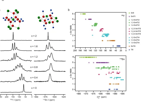
Sn/Ti disorder in pyrochlore ceramics and F substitution into hydrous
minerals.[9,11,69,80-86] A better approximation for an aperiodic structure (particularly for
low level disorder) can be obtained by using a repeating crystal composed of “supercells”,
as shown in Figure 9c, where the supercell is chosen to be sufficiently large to minimise
the effect of any structural change on the neighbouring cells. It should also be noted that
using a supercell increases the number of atoms to be treated explicitly, thereby increasing