PROBLEMS
E. K. Burke , A. J. Eckersley , B. McCollum
, S. Petrovic , R. Qu
University of Nottingham, Nottingham NG8 1BB, UK
Queen’s University of Belfast, Northern Ireland
Abstract
A large number of heuristic algorithms have been developed over the years which have been aimed at solving examination timetabling problems. However, many of these algorithms have been developed specifically to solve one partic-ular problem instance or a small subset of instances related to a given real-life problem. Our aim is to develop a more general system which, when given any exam timetabling problem, will produce results which are comparative to those of a specially designed heuristic for that problem. We are investigating a Case based reasoning (CBR) technique to select from a set of algorithms which have been applied successfully to similar problem instances in the past. The assump-tion in CBR is that similar problems have similar soluassump-tions. For our system, the assumption is that an algorithm used to find a good solution to one problem will also produce a good result for a “similar” problem. The key to the success of the system will be our definition of similarity between two exam timetabling prob-lems. The study will be carried out by running a series of tests using a simple Simulated Annealing Algorithm on a range of problems with differing levels of “similarity” and examining the data sets in detail. In this paper an initial inves-tigation of the key factors which will be involved in this measure is presented with a discussion of how the definition of good impacts on this.
Keywords: Timetabling, Heuristic Search
1.
Introduction
con-straints into account regarding driver working hours, starting and ending points for vehicles and many other constraints which are relevant to the individual timetable. These types of timetable give a good overview of the key elements of a generic timetabling problem - namely that a set of events must be sched-uled to certain times whilst obeying a number of rules, known as constraints.
Timetabling is mainly concerned with the assignment of events to timeslots subject to constraints. There is not necessarily any allocation of resources to the events timetabled. In reality however, it is almost always required to know that there are sufficient resources available for the given event to take place at its specified time as well as which resources are allocated. More formally, Wren [15], says:
“Timetabling is the allocation, subject to constraints, of given resources to ob-jects being placed in space time, in such a way as to satisfy as nearly as possible a set of desirable objectives”
The University timetabling problem can be divided into two areas, these be-ing course (or lecture) timetablbe-ing and examination timetablbe-ing. In this paper we will consider only the exam timetabling problem which will be described in more detail in Section 2.
Some recent research [6] has focused on hyper-heuristic methods applied to timetabling problems with the aim being to develop a more general approach than producing problem-specific heuristics. These hyper-heuristics work on a level of abstraction above that of standard heuristics, to select the best from a selection of lower-level heuristic algorithms. The focus of this paper will be on a case based reasoning system for exam timetabling problems which works at the level of a hyper-heuristic. Case-based reasoning (CBR) has been ap-plied directly to University course timetabling problems [2], [3] successfully and the next logical step is to consider using CBR at a higher level of ab-straction to select from a set of previously used heuristics to solve any given timetabling problem. A more detailed description of case based reasoning and its use within our project as a heuristic selector will be given in Section 3.
The focus of this paper is on investigating the data sets in more detail to discover some of the key elements that will define how well an algorithm per-forms when applied to the problem. For this purpose, we will be using a simple Simulated Annealing algorithm to produce results on a number of variants of the given data sets. A brief description of this algorithm will be given in Sec-tion 4. Our analysis of the data sets used and our plans for further analysis are reported in Section 5.
2.
Examination Timetabling
are a large number of variations on the theme of exam timetabling with dif-ferent institutions having difdif-ferent requirements and constraints (see [1]). In some cases, there will be a limited number of rooms into which exams must be placed whilst in others this may not be an issue. Similarly, some institutions will have large amounts of inter-departmental modular courses whereas others will offer more strictly department-based courses meaning fewer conflicts with exams from other departments.
In the most basic timetabling problem, every exam timetabling problem has
a set
of exams and a set
of periods into which all exams must be scheduled. A number of other side-constraints must also be either fully or partially satisfied to form the timetable. Hard constraints are those which must be satisfied in order for the timetable to be feasible. The most important of these are:
any pair of exams,
, with students in common cannot both be as-signed to the same period
.
there must be sufficient resources available in each period,
, for all the exams timetabled.
Soft constraints are those whose violation should be minimised in order to
produce the best timetable. Unlike hard constraints these are not essential, but soft constraint satisfaction provides a measure of how good a timetable is. Soft constraints vary greatly between institutions. Some of the most common ones are [1], [6]:
Time assignment - An exam may need to be scheduled in a specific
pe-riod
Time constraints between events - One exam may need to be scheduled
before/after another
Spreading events over time - Students should not have exams in
consec-utive periods or two exams within periods of each other
Resource assignment - An exam must be scheduled into a specific room
which have been developed are very problem-specific and cannot be used to find high quality solutions to a wide range of problem instances. In general though, no one algorithm will give best results for all exam timetabling prob-lems to which it is applied. Some algorithms will perform well on one subset of problems whilst fairing fairly poorly when different constraints are introduced. Our aim is to develop a system which can select the best from a range of heuristics when given a new problem so that good results can be obtained across a wide spectrum of problem instances. A case based approach requires a large amount of knowledge of past performance of algorithms on particular problems in order to make an intelligent selection of which algorithm should perform best on the new problem. Each exam timetabling problem has a
land-scape which is defined on its horizontal plane by the set of all feasible
so-lutions1 with the vertical aspect defined at each of the points representing a solution by the objective function for the problem – this gives the measure of how good the solution is based on certain criteria. How successful a given algorithm is at finding a good solution (a good local minima, or ideally the global minima) therefore depends on how well it traverses this landscape to escape from local minima and navigate towards better ones whilst providing a good coverage of the search space. If we can show that a given algorithm traverses two different problem landscapes equally well, we can consider the two landscapes to be similar and the key elements which define the shapes of these landscapes to form good measures of similarity.
3.
Case Based Reasoning (CBR)
Case based reasoning is motivated by a process used by humans, often sub-consciously when making everyday decisions. CBR is a process of learning from previous experiences, storing that knowledge in a useful manner and re-trieving it to reuse when a similar situation presents itself later. Kolodner [12] gives an in-depth explanation of CBR, its applications and the key ideas behind it, of which a brief summary is presented here.
A Case is a ‘contextualised piece of knowledge which represents an expe-rience.’ Each case contains knowledge about one previous experience, repre-sented and indexed in such a way that it can be retrieved easily when a similar situation is encountered. The cases are all indexed within a case base, with each case adding a separate piece of knowledge to the system.
The motivation underlying case based reasoning is that similar problems
have similar solutions. When a new problem is encountered, its key
descrip-tors will be noted and matched against those of problems in the case base using some measure of similarity. The most similar case(s) will be retrieved
to be re-used for the new problem. In some cases, the exact same solution can be re-used, but more often there will be differences between the new problem and the retrieved problem which must be reconciled. In these situations, the retrieved solution must be adapted before it can be used to solve the new prob-lem. An important aspect of any successful CBR system is the feedback which the system receives regarding how good the retrieved solution was for the new problem. If the solution was good, then the new problem may be added to the system if it contains any new information which may be useful in the future. If the solution was bad, however, the indexing for the retrieved case needs to be reconsidered so that this case would no longer be regarded as similar to the new case. Feedback about failure is just as important as feedback about success for the system to function to the highest standard. Learning from past mistakes and making sure not to repeat them provides very valuable knowledge.
For example, CBR is used very successfully in the medical field for diag-nosing illnesses. Key descriptors of patient’s symptoms and other important information is stored as a case in the case base. When a new patient arrives with similar symptoms, the case will be retrieved and the differences between the two must be reconciled (for instance a difference in blood pressure or heart beat), then the old case may be adapted to find a diagnosis for the new patient.
CBR for Scheduling
CBR has been discussed and applied directly to scheduling problems by Burke et al. [2], [3] (course timetabling), Miyashita and Sycara [14] (job shop scheduling) and MacCarthy [13] (general scheduling) amongst others. Burke et al. use cases from the case base to help construct a solution to a new prob-lem by using graph isomorphism of attribute graphs. The main issues they considered are:
how to represent complex timetabling problems how to organise the case base
how to measure similarity between two problems to retrieve the most useful case
how to adapt the retrieved solution for the new problem. These are discussed in more detail in [2] and [6].
Our CBR system for Exam Timetabling
One of the next major areas for CBR is to work on the level of a hyper-heuristic. This would select, from a range of previously used heuristics, the
a system is how we define the best algorithm to be used for the new problem. Applying the general theory behind CBR, we assume that an algorithm which performs well on one problem will also perform well on a similar problem. Therefore the main area of consideration is how two problems can be measured as similar in such a way that this reasoning holds.
Each case in our case base will consist of a problem definition together with an algorithm used to successfully solve the problem. A standard format for defining exam timetabling problems has been developed for use in the system to enable matching of any two problems to measure their similarity. Once a new problem is presented to the system, the matching process will retrieve the most similar problem from the case base along with the most successful algo-rithm(s) used to solve that problem. Based on how similar the retrieved case is to the new one, the retrieved algorithm may be adapted by tuning its parameters in some way or by using a hybrid of more than one retrieved algorithm.
The development of such a system provides a large number of research ar-eas. Of these, the biggest is the definition of similarity which is the one we consider here. In this paper we consider the key elements in the definition of an exam timetabling problem and work towards a definition for similarity based on which features seem to have the biggest effect on how successful an algorithm is. Of course, for our purposes, two similar timetabling problems would mean that the same algorithm would be suitable for both problems. Two problems would be dissimilar if a particular algorithm/heuristic worked very well on one problem but not on the other. Essentially this means that two sim-ilar problems should have a simsim-ilar landscape as seen from the point of view of the algorithm operating on these landscapes. Given the nature of the do-main in question, there are a potentially infinite number of simple and more complex statistical measures which could be used to compare two given exam timetabling problems. Many of these will actually have very little impact on the success of a given algorithm on the problem, whereas others could be ma-jor factors in how well the algorithm navigates the search space to find a good solution. Our aim here is to study the make up of the data sets themselves to examine the effects of some of the more likely problem descriptors on the solutions produced by our Simulated Annealing Algorithm.
4.
Testing Algorithm
Ultimately our aim is to have a large number of different types of algorithms in our system which have been applied to a number of different problems of varying difficulty. Each (problem, algorithm) pair which produces a good re-sult will be stored as a case with some problems possibly being duplicated if more than one algorithm provides high quality results. Initially, however, we plan to start building up a case base from the simplest algorithms and de-velop them and introduce more complex algorithms in future research work. With our initial algorithms we are running a series of tests on real life data sets from a wide variety of institutions to provide a better idea of how the problem definition affects the algorithm’s behaviour and leads towards a definition of similarity.
Our definition of similarity, , between two cases, ! and!" has the fol-lowing form:
$#% "'& )(
#
+* ,
#-./ 10
./2
-&%&
where:
(
#
& and
,
#
& are functions which will be tuned as more cases are added to the case base
is the number of features in the similarity measure ./
and./2
are the values of the3 th feature of cases and " respec-tively
The main purpose of the tests we are carrying out firstly with our simple algorithms and later with more complex algorithms is to eliminate the features in the problem definition which have no effect on the behaviour of the algo-rithm and to see how stable certain algoalgo-rithms are regarding other features - for instance, how large a change in a particular feature is needed to have a signifi-cant affect on the quality of solution produced by a particular algorithm when compared to another algorithm.
Given the complex nature of the problem landscapes involved it is unlikely that our tests will produce any concrete, quantitative results regarding exactly which parts of the problem definition have what effect on the algorithm per-formance, but we aim to acquire as much qualitative information as possible to enable us to make value judgements on which features to include in our simi-larity measure and what type of tolerance to allow for each individual feature in order for two cases to be considered similar based on that feature. The tol-erance for each feature will be defined and tuned as the set of functions,
We use a largest degree graph colouring heuristic with backtracking to pro-vide an initial feasible solution2 for our initial algorithm which will then only explore the set of feasible solutions. The simple neighbourhood used is defined by all solutions in which one exam is moved to a new time slot. The objec-tive function to be optimised for our problems is discussed in Sections 5 and 6 whilst a brief description of our Simulated Annealing algorithm is given in the following subsection.
Simulated Annealing
Our Simulated Annealing algorithm selects both exam,
, and period,
, at random, checking whether moving exam
to period
is a legal move3. If not, a maximum of 9 more periods are tested to find a feasible move, otherwise a new exam is randomly chosen and the process repeated. This move is then accepted or rejected using the standard probabilistic acceptance criteria of Simulated Annealing (see e.g. [11]) with improving moves always accepted and worse moves accepted with decreasing probability based on the geometric cooling schedule. The starting temperature and cooling schedule are initially chosen arbitrarily and tuned based on results.
Results may be improved by limiting exam selection to only those involved in second-order conflicts, although this will also reduce the range of the search space investigated. Hill Climbing could also be incorporated in some way to ensure that local minima are found before the search moves away to a new area, (in a similar manner to a memetic algorithm). For the purposes of this paper, however, we used a very simple implementation which still produces results of an acceptable quality since our aim isn’t to compare the absolute results with those obtained by other algorithms at this stage.
5.
Data Sets
Initially, all our tests have been carried out on Carter’s Benchmark data sets [9] without any soft constraints. The objective function used by Carter is based only on the sum of proximity costs as defined below:
46587 :9;
;
5
=<8> ?
@
where465
is the weight given to clashing exams scheduled<
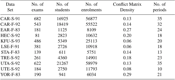
periods apart. Initially the most obvious problem features have been identified and are presented in Tables 1 and 2, although many of these are likely to have only a small effect on the performance of algorithms. As well as those shown, there
2with all hard constraints satisfied
Table 1. Features for Carter Data Sets
Data No. of No. of No. of Conflict Matrix No. of
Set exams students enrolments Density periods
CAR-S-91 682 16925 56877 0.13 35
CAR-F-92 543 18419 55522 0.14 32
EAR-F-83 181 1125 8109 0.27 24
HEC-S-92 81 2823 10632 0.20 18
KFU-S-93 486 5349 25113 0.06 20
LSE-F-91 381 2726 10918 0.06 18
STA-F-83 139 611 5751 0.14 13
TRE-S-92 261 4360 14901 0.18 23
UTA-S-92 622 21267 58979 0.13 35
UTE-S-92 184 2750 11793 0.08 10
YOR-F-83 190 941 6034 0.29 21
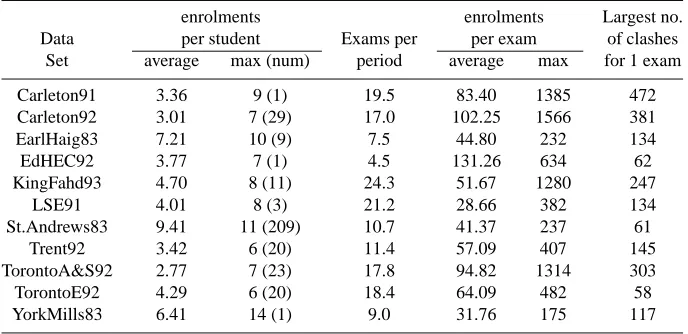
are a large number of statistical measures which can be applied to the data sets in order to determine the distributions of exams and enrolments amongst students. Table 2 shows that there is a wide variation in the average number of enrolments per student between the different data sets and the maximum number of exams that any student is taking. A statistical analysis of these enrolments should give an idea as to how well spread they are away from the average and whether there are any significant anomalies within any of the data sets. Such analysis should provide further basis for our study of similarity measures.
In this paper, however, we look in more detail at the student enrolments themselves and examine the effect they have on the structure of the problem. We also consider how big an impact the objective function has on these mea-sures of similarity.
6.
Analysis of Data Sets - Results & Conclusions
Table 2. Features for Carter Data Sets
enrolments enrolments Largest no.
Data per student Exams per per exam of clashes
Set average max (num) period average max for 1 exam
Carleton91 3.36 9 (1) 19.5 83.40 1385 472
Carleton92 3.01 7 (29) 17.0 102.25 1566 381
EarlHaig83 7.21 10 (9) 7.5 44.80 232 134
EdHEC92 3.77 7 (1) 4.5 131.26 634 62
KingFahd93 4.70 8 (11) 24.3 51.67 1280 247
LSE91 4.01 8 (3) 21.2 28.66 382 134
St.Andrews83 9.41 11 (209) 10.7 41.37 237 61
Trent92 3.42 6 (20) 11.4 57.09 407 145
TorontoA&S92 2.77 7 (23) 17.8 94.82 1314 303
TorontoE92 4.29 6 (20) 18.4 64.09 482 58
YorkMills83 6.41 14 (1) 9.0 31.76 175 117
the various problem descriptors – for instance, what effect would removing 10 students from a given data set have on enrolments and the conflict matrix4?
Removing redundancy from Data Sets
The input files for the Carter Data sets consist of sets of # <ACBED
A
EFHG & pairs representing one enrolment for a given student. Further enrolments for the same student are recorded in the same fashion on following lines. It was observed that in many of the data sets there were a significant number of stu-dents who had only one enrolment. These stustu-dents, it was decided have no impact on the difficulty of the exam timetabling problem or its landscape since they are involved in no clashes and therefore they do not have any effect on the end result – they can sit their one exam equally easily whenever it is sched-uled since capacity constraints are not considered. Our first new data sets were then produced by removing all those students with a single enrolment from the problem and running the Simulated Annealing algorithm on this reduced student set. Table 3 shows some of the key statistics of these data sets for 3 of the Carter problems and the results confirm that removing these students has no impact on the final result,5 as calculated by dividing the total penalty for
Table 3. Results using Simulated Annealing on 3 Carter Data Sets with all single enrolment students removed
Data Students Total Average Standard Result
Set enrolment enrolment Deviation
Carleton91 16925 56877 3.36 1.57 6.84
Carleton91 minus 13516 53468 3.96 1.15 6.82
Trent92 4360 14901 3.42 1.41 11.32
Trent92 minus 3693 14234 3.85 1.15 11.40
EdHEC92 2823 10632 3.77 1.44 15.33
EdHEC92 minus 2502 10311 4.12 1.11 15.50
the timetable by the number of students6. The reduced data sets are denoted by adding ‘ minus’ to the original data set in the table.
The main points to note from the results in Table 3 are that, whilst removing a relatively large number of students from the problem ( 20% in the case of the Carleton91 data set) there is no effect at all on the final timetable produced. However, it does have a fairly noticeable effect on many of the other measures which we put forward as being possible factors in a similarity measure – many of which would be statistical measures based on the number of students or enrolments and ratios involving these two factors. From the point of view of the algorithm operating on the problems, the Carleton91 data set and its reduced Carleton91 minus data set are identical and should therefore be regarded as
similar (or indeed identical) from a Case based reasoning ‘heuristic selector’
perspective. This result shows us that a fairly detailed analysis of the data sets and what the students in these data sets actually add to the overall problem is necessary before we start to consider any measures of similarity between two data sets.
On the face of it, using the measures shown in Table 3, the reduced data sets are not very similar to their equivalent complete sets at all, when com-paring the students, enrolments, average enrolment and the standard deviation of the enrolments, yet as we have shown, the reduced sets should be consid-ered identical to their complete sets from the point of view of selecting an algorithm to solve the problems. Therefore, if these factors are still to be considered when investigating measures of similarity, we need to make sure that we have reduced our data sets to their minimum definition by removing any redundancy before comparing them for similarity. For example, if
Car-6The results for the reduced sets are calculated by dividing by the number of students in the equivalent full
leton91 minus formed part of a case7within our case base and the Carleton91 data set were input to the system to find a match, it would be pre-processed before the matching process to remove the single enrolment students, then the Carleton91 minus case would be retrieved as an exact match and its corre-sponding algorithm used to solve the Carleton91 set.
This result prompted a variety of further research questions which needed to be examined further. Amongst these were the questions of how a ‘good’ timetable is defined and whether there is any more redundancy which can be removed from the data sets before the matching process.
A measure for reporting results for the Carter data sets is Average penalty
per student which is calculated by taking the overall penalty for the whole
timetable, defined by the objective function, and dividing by the number of students in the data set. However, in absolute terms this number means very little since, as shown above, the number of students in a data set is not a very good measure of similarity. It can be argued that since 3409 students in the Carleton91 data set are only taking 1 exam and therefore add no penalty to the overall timetable, that these students shouldn’t be included in the Average
penalty per student measure. In an extreme case, a data set could contain 50%
of students who take only 1 exam - in this case, dividing the total penalty for the timetable by all the students would give a result twice as good as if you ignore half of the students who add nothing to the “difficulty” of the problem - yet the timetable itself would be identical in both cases. In itself this isn’t a major concern since the results produced for these data sets are only used for comparison purposes against each other so as long as everyone uses the same measure, algorithms can be compared to see which is better. These observa-tions did, however lead us in the direction of our further research into the issue of more redundancy in the data sets.
Examining subsets of the Data Sets
Having removed all the single enrolment students from the data sets and witnessed the impact this had on the results and potential similarity measures, we decided to see if there was any more redundancy within the problem defini-tion for these sets. The next obvious area to investigate was the issue of repeat students, i.e. 2 or more students with the exact same enrolments. These are very common in real-life problems given that students on the same course tend to have many or all exams in common. In addition to exact repeat students, there are also students whose enrolments form a subset of 1 or more other stu-dents. With the student enrolment file sorted in descending order of number of enrolments we could now read in students one at a time and remove any
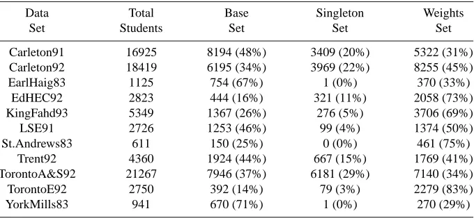
Table 4. Percentages and numbers of students in the Base Set, Singleton Set and Weights Set for Carter Data Sets
Data Total Base Singleton Weights
Set Students Set Set Set
Carleton91 16925 8194 (48%) 3409 (20%) 5322 (31%)
Carleton92 18419 6195 (34%) 3969 (22%) 8255 (45%)
EarlHaig83 1125 754 (67%) 1 (0%) 370 (33%)
EdHEC92 2823 444 (16%) 321 (11%) 2058 (73%)
KingFahd93 5349 1367 (26%) 276 (5%) 3706 (69%)
LSE91 2726 1253 (46%) 99 (4%) 1374 (50%)
St.Andrews83 611 150 (25%) 0 (0%) 461 (75%)
Trent92 4360 1924 (44%) 667 (15%) 1769 (41%)
TorontoA&S92 21267 7946 (37%) 6181 (29%) 7140 (34%)
TorontoE92 2750 392 (14%) 79 (3%) 2279 (83%)
YorkMills83 941 670 (71%) 1 (0%) 270 (29%)
duplicate students from the data set. These would also include any students whose clashes had already been recorded by earlier students. For example, if a student with enrolmentsF ,I andJ is followed by 3 students with enrolments #%F I & , #%F J & and #%I J & respectively, the last 3 students can all be discarded from the data set since their clashes were recorded by the first student.
In removing these duplicate students, it was noted that their absence would have an impact on the final penalty for the timetable, unlike the removal of the single enrolment students. The reason for this being that the objective function used weights all clashes by the number of students involved in the clash so that clashes with a large number of students are a higher priority to spread well apart than those with only a few students. Therefore, duplicate students do add to the overall penalty of the timetable. Despite this, it was still considered worthwhile to remove them to examine the remaining set. The justification for this being that while duplicate students do contribute to the problem definition, they only do so relative to the objective function used to define a good timetable. In terms of the hard constraints they don’t alter the problem and we are interested to examine the effect of the objective function on measuring the similarity of problems. The results obtained are shown in Table 4.
The Singleton Set is the set of single enrolment students removed initially, the weights set is the set of duplicate students (as defined above) whilst the
Base Set is the set of students remaining after all students in both the Singleton
the set of feasible solutions to the larger problem whilst the Weights set is so named because the students in that set simply add weights to the already existing clashes.
One major point to note from the 3 sets is that whilst the Singleton set can be taken on its own, the Base set and the Weights set are less easy to split in a meaningful way since the Base set does still include a number of weights on various edges. This is due to the fact that only students whose entire set of clashes had already been noted were removed to the weights set, leaving those who have only some of their clashes already noted to be included in the Base set as their remaining clashes add new information to the set. If any single student is removed from the Base set, the definition of the feasible problem will change because one or more clashes will be lost. Removing students from the weights set, whilst keeping the rest for the problem would retain the same basic problem definition, but will change the weightings and therefore the bias of the clashes when the Simulated Annealing algorithm operates on the problem.
Using the objective function given by Carter [9] to provide results for the problems therefore, it is difficult to use the information discovered by splitting the data sets up in this way due to the above mentioned weights included in the Base set. However, we decided that this splitting up of the data sets into subsets looked promising as a potentially important factor in comparing dif-ferent data sets since the percentage of students forming the base set varies greatly between data sets - for instance, the fact that only 14% of the 2750 students in the TorontoE92 data set are required to define the problem in terms of feasibility compared to 71% of the 941 YorkMills83 students is a significant difference.
As a result of this we decided to re-consider the definition of a good timetable as proposed by Carter’s objective function. From the point of view of a student taking the exams, their criteria for how important particular clashes are could include a variety of individual reasons based on how difficult they find certain exam schedules to be, but none of these can be taken into account in the overall timetable since they are individual preferences. However, the number of other students involved in a particular clash is completely unimportant to any indi-vidual student. Whether they are the only student doing two particular exams or whether there are 100 other students also taking those two exams does not matter to them and therefore weighting clashes by the number of students in-volved in the clash gives what could be considered an unbalanced bias in the timetable.8 Exams with many students in common may often be easier ones
8This is a highly debatable issue and ours is just one perspective on how to consider what a "good" timetable
from the point of view of the student having to revise for and sit the exam. Conversely, exams with relatively few students may be more specialised and difficult from a student’s perspective - students would need more intensive revi-sion for such exams if they are scheduled close together. Weighting the former far more than the latter would result in the ‘easier’ exams being spread well apart for lower overall penalty whilst the ‘harder’ exams for the students may be relatively close together since their total penalty in the timetable is small.
Using this justification we decided that removing all student weightings from the objective function and weighting clashes purely by the number of periods apart in the timetable would produce what could be considered a “fair” timetable from the student’s point of view and would vastly simplify the prob-lem from the point of view of the data sets, meaning that we could totally dis-card all the Weights sets and concentrate purely on the Base Sets of students which define the conflict matrix9.
Experiments carried out on the whole data set and on just the base set of each data set using such an objective function with no student weightings showed, as expected, that the results produced (the total penalty for the timetable as de-fined by the new objective function) were identical for the full set of students and for the base set. The conclusion to be drawn from this is that the definition of a good timetable can have a huge impact on the relevant statistics of a given data set. Using our new definition of good, the 2750 student TorontoE92 prob-lem is identical to the 392 student TorontoE92 Base Set probprob-lem and therefore, should be matched as such by our similarity measure.
Conclusions and Further Work
To summarise the main conclusions found in our work so far, in order to use any of the statistical measures produced for a given data set as a measure of similarity within our CBR system, we must first strip away any redundancy from the data based on the particular objective function used and use only the minimum set of students which adequately define the problem to match against data sets existing in the database. Our experiments have shown that, depending on how you define a good timetable, the same data set can be split up and stripped down into very different looking data sets, but which are actually identical for the purposes of running an algorithm to find the best results.
Our future work will continue with this analysis and introduce a number of new statistical measures of the data sets, examining their distributions and seeing how the removal of sets of students or exams from the data set changes the problem. As has been shown in this paper, removing students at random,
similarity - our justification being that purely from a student’s perspective, the number of students involved in any given clash is not a relevant factor for the scheduling of exams
even a large number, from the original data set may have no impact at all on the problem, whereas removing just 1 or 2 students from the Base Set can completely change the problem definition and difficulty. We will also carry out tests of the same kind using our other algorithms as well as examining the effect on one optimisation function of optimising results using a different function. - i.e. we will output the results from two functions whilst optimising the solution using only one of them and observe how the results from the other function alter.
References
[1] Burke, E.K., Elliman, D.G., Ford, P., Weare, R.F. Examination Timetabling in British Uni-versities - A Survey, in [7], pp 76-92.
[2] Burke, E.K., MacCarthy, B., Petrovic, S., Qu, R. Structured cases in case-based reasoning - re-using and adapting cases for time-tabling problems. Knowledge-Based Systems 13 (2000) pp 159-165.
[3] Burke, E.K., MacCarthy, B., Petrovic, S., Qu, R. Case-Based Reasoning in Course Timetabling: An Attribute Graph Approach. Proceedings of the 4th. International Con-ference on Case-Based Reasoning, ICCBR-2001, Vancouver, Canada, 30 July - 2 August 2001. Springer, Lecture Notes in Artificial Intelligence vol. 2080, pp. 90-104
[4] Burke, E.K. and Erben, W. (eds). PATAT 2000 - Proceedings of the 3rd international con-ference on the Practice and Theory of Automated Timetabling.
[5] Burke, E.K. and Erben, W. (eds). The Practice and Theory of Automated Timetabling III, volume 2079 of Lecture Notes in Computer Science. Springer-Verlag, 2001.
[6] Burke, E.K. and Petrovic, S. Recent Research Directions in Automated Timetabling. Euro-pean Journal of Operational Research - EJOR, 140/2, 2002, 266-280
[7] Burke, E.K. and Ross, P., editors. Practice and Theory of Automated Timetabling, volume 1153 of Lecture Notes in Computer Science. Springer-Verlag, 1996.
[8] Carter, M. W. and Laporte, G. Recent Developments in Practical Examination Timetabling In [7], pp 3-21.
[9] Carter, M. W., Laporte, G. and Lee, S. Y. Examination timetabling: Algorithmic strategies and applications. Journal of Operational Research Society, 74:373-383, 1996.
[10] Erben, W. A Grouping Genetic Algorithm for Graph Colouring and Exam Timetabling. In [5], pp 132-158
[11] Henderson, D., Jacobson, S. H. and Johnson, A. W. The Theory and Practice of Simulated Annealing. In Glover, F. and Kochenberger, G. A. (eds), Handbook of Metaheuristics, pp. 287-319.
[12] Kolodner, J. Case-Based Reasoning. Morgan Kaufmann Publishers, Inc. San Mateo.
[13] MacCarthy, B. and Jou, P. Case-based reasoning in scheduling. In M. K. Khan, C. S. Wright (Eds.), Proceedings of the Symposium on Advanced Manufacturing Processes, Systems and Techniques. (AMPST96), MEP Publications, 1996, pp. 211-218.