Revised
Proof
DOI 10.1007/s00466-014-1032-2O R I G I NA L PA P E R
A hysteretic multiscale formulation for nonlinear dynamic
analysis of composite materials
S. P. Triantafyllou · E. N. Chatzi
Received: 19 July 2013 / Accepted: 7 April 2014
© The Author(s) 2014. This article is published with open access at Springerlink.com
Abstract A new multiscale finite element formulation 1
is presented for nonlinear dynamic analysis of heteroge-2
neous structures. The proposed multiscale approach utilizes 3
the hysteretic finite element method to model the micro-4
structure. Using the proposed computational scheme, the 5
basis functions, that are used to map the micro-6
displacement components to the coarse mesh, are only eval-7
uated once and remain constant throughout the analysis pro-8
cedure. This is accomplished by treating inelasticity at the 9
micro-elemental level through properly defined hysteretic 10
evolution equations. Two types of imposed boundary condi-11
tions are considered for the derivation of the multiscale basis 12
functions, namely the linear and periodic boundary condi-13
tions. The validity of the proposed formulation as well as 14
its computational efficiency are verified through illustrative 15
numerical experiments. 16
Keywords Heterogeneous materials·Multiscale finite 17
elements·Hysteresis·Nonliner dynamics 18
1 Introduction 19
Composite materials have long been utilized in construc-20
tion and manufacturing in various forms. Nowadays, their 21
scope of applicability spans a large area including, though
S. P. Triantafyllou (
B
)School of Engineering and Design, Brunel University, Kingston Lane, Uxbridge UB8 3PH, UK
e-mail: [email protected] E. N. Chatzi
Institute of Structural Engineering, ETH Zürich, Stefano-Franscini-Platz 5, 8093 Zürich, Switzerland e-mail: [email protected]
not limited to the aerospace, automobile and sports indus- 22 tries [28]. Their appeal lies in the fact that composites exhibit 23 some enhanced mechanical properties, such as high strength 24 to weight ratio, high stiffness to weight ratio, high damp- 25 ing, negative Poisson’s ratio and high toughness. In the 26 field of Civil Engineering, composite materials are used 27 either in the form of fiber reinforcing or more recently 28 as textile composites in various applications such as retro- 29 fitting and strengthening of damaged structures [11], or sup- 30 porting cables for cable stayed bridges and high strength 31 bridge decks [26] amongst many others. This vast and mul- 32 tidisciplinary implementation of composites results in the 33 need for better understanding of their mechanical behav- 34 iour. Research efforts are oriented towards further improving 35 the mechanical properties of composites while at the same 36 time alleviating some of their disadvantages such as high 37 production/ implementation costs and damage susceptibility 38
[52]. 39
Revised
Proof
and distributions of heterogeneities that the material consists57 of. 58
The derivation of reliable numerical models for the sim-59
ulation of mechanical processes occurring across multiple 60
scales can aid both the design and/or optimization of new 61
composite systems. Using appropriate modelling assump-62
tions accounting for plasticity and damage [38], estimates 63
on the damage susceptibility of composites can be read-64
ily derived and parametric models can be established where 65
micro-material properties are identified based on experimen-66
tally measured quantities. 67
Modelling of structures that consist of composites could 68
be accomplished using the standard finite element method 69
[65]. However, a finite element model mesh accounting for 70
each micro-structural heterogeneity would require signifi-71
cant computational resources (both in CPU power and stor-72
age memory). In general, the computational complexity of a 73
finite-element solution procedure is of the order ofO
n3z/2
74
wherenz is the number of degrees of freedom of the
under-75
lying finite element mesh [37]. Therefore, the finite ele-76
ment scheme is usually restricted to small scale numeri-77
cal experiments of a representative volume element (RVE) 78
[1,53]. 79
To properly capture the micro-structural effects in the 80
large scale more refined methods have been developed. 81
Instead of implementing the standard finite element method, 82
upscaled or multiscale methods have been proposed to 83
account for such types of problems, therefore significantly 84
reducing the required computational resources [36,59,67]. 85
Upscaling techniques rely on the derivation of analytical 86
forms to describe a coarser (i.e. large scale) model based 87
on smaller scale properties [40]. Usually this is accomplished 88
by analytically defining a homogenized constitutive law from 89
the individual constitutive relations of the constituents. Thus, 90
a continuous mathematical model that is problem depen-91
dent replaces the fine scale information. On the other hand, 92
multiscale methods use the fine scale information to formu-93
late a numerically equivalent problem that can be solved in 94
a coarser scale, usually through the finite element method 95
[2,55]. An extensive review on the subject can be found in 96
[33]. 97
In general, multiscale methods can be separated in two 98
groups, namely multiscale homogenization methods [45] and 99
multiscale finite element methods (MsFEMs) [20]. Within 100
the framework of the averaging theory for ordinary and par-101
tial differential equations, multiscale homogenization meth-102
ods are based on the evaluation of an averaged strain and cor-103
responding stress tensor over a predefined space domain (i.e. 104
the RVE) [5]. Amongst the various homogenization meth-105
ods proposed [25], the asymptotic homogenization method 106
has been proven efficient in terms of accuracy and required 107
computational cost [61]. 108
However, these methods rely on two basic assumptions, 109 namely the full separation of the individual scales and the 110 local periodicity of the RVEs. In practice, the heterogeneities 111 within a composite are not periodic as in the case of fiber- 112 reinforced matrices . In order to adapt to general heteroge- 113 neous materials, the size of RVE must be sufficiently large 114 to contain enough microscopic heterogeneous information 115 [3,54], thus increasing the corresponding computational cost. 116 Furthermore, in an elasto-plastic problem, periodicity on the 117 RVEs also dictates periodicity on the damage induced which 118 could result in erroneous results. 119 The MsFEM is a computational approach that relies on 120 the numerical evaluation of a set of micro-scale basis func- 121 tions. These are used to map the micro-structure informa- 122 tion onto the larger scale. These basis functions depend both 123 on the micro-structural geometry and constituent material 124 properties. Therefore, the heterogeneity can be accounted 125 for through proper manipulation of the underlying finite ele- 126 ment meshes defined at different scales. MsFEM was first 127 introduced in [31] although a variant of the method was 128 earlier introduced in [7] for one-dimensional problems and 129 later for the multi-dimensional case [6]. Along the same 130 lines, domain-decomposition [66] and sub-structuring [68] 131 approaches have also been introduced for the solution of elas- 132 tic micro-mechanical assemblies. 133 Although MsFEMs have been extensively used in linear 134 and nonlinear flow simulation analysis [19,27] the method 135 has not been implemented in structural mechanics problems. 136 This is attributed to the inherent inability of the method to 137 treat the bulk expansion/ contraction phenomena (i.e. Pois- 138 son’s effect). To overcome this problem, the enhanced mul- 139 tiscale finite element method (EMsFEM) has been proposed 140 for the analysis of heterogeneous structures [62]. EMsFEM 141 introduces additional coupling terms into the fine-scale inter- 142 polation functions to consider the coupling effect among dif- 143 ferent directions in multi-dimensional vector problems. The 144 method has been also extended to the nonlinear static analy- 145 sis of heterogeneous structures [63]. Recently, the geometric 146 multiscale finite element method was introduced [14] along 147 with a novel approach for the numerical derivation of dis- 148 placement based shape functions for the case of linear elastic 149
problems. 150
Revised
Proof
nonlinear dynamic analysis, where a time integration scheme161
is also required on top of the iterative procedure [30]. 162
In this work, a modified multiscale finite element analysis 163
procedure is presented for the nonlinear static and dynamic 164
analysis of heterogeneous structures. In this, the evaluation 165
of the micro-scale basis functions is accomplished within 166
the hysteretic finite element framework [56]. In the hys-167
teretic finite element scheme, inelasticity is treated at the 168
element level through properly defined evolution equations 169
that control the evolution of the plastic part of the deformation 170
component. Using the principle of virtual work, the tangent 171
stiffness matrix of the element is replaced by an elastic and 172
a hysteretic stiffness matrix both of which remain constant 173
throughout the analysis. 174
Along these lines, a multi-axial smooth hysteretic model 175
is implemented to control the evolution of the plastic strains 176
that is derived on the basis of the Bouc–Wen model of hys-177
teresis [10]. The smooth model used in this work accounts 178
for any kind of yield criterion and hardening law within 179
the framework of classical plasticity [38]. Smooth hysteretic 180
modelling has proven very efficient with respect to classi-181
cal incremental plasticity in computationally intense prob-182
lems such as nonlinear structural identification [12,35,43], 183
hybrid testing [13] and stochastic dynamics [58]. Further-184
more, the proposed hysteretic scheme can be extended to 185
account for cyclic damage induced phenomena such as stiff-186
ness degradation and strength deterioration [4,22]. The ther-187
modynamic admissibility of smooth hysteretic models with 188
stiffness degradation has proven on the basis of an equiva-189
lence principle to the endochronic theory of plasticity [21]. 190
However, such concepts are beyond the scope of this work. 191
The present paper is organized as follows. The smooth 192
hysteretic model together with the hysteretic finite element 193
scheme that form the basis of the proposed method are 194
described in Sect.2. In Sect.3, the enhanced multiscale finite 195
element method (EMsFEM) is briefly described. In Sect.4, 196
the proposed hysteretic multiscale finite element method is 197
presented. The method used for the solution of the governing 198
equations at the coarse mesh is described in Sect.5. The lat-199
ter is based on the simulation of the governing equations of 200
motion in time using the Newmark direct-integration method 201
[17]. In Sect.6a set of benchmark problems is presented to 202
verify both the accuracy and the efficiency of the proposed 203
multiscale formulation. 204
2 Hysteretic modelling 205
2.1 Multiaxial modelling of hysteresis 206
Classical associative plasticity is based on a set of four 207
governing equations, namely the additive decomposition of 208
strain rates, the flow rule, the hardening rule and the consis- 209 tency condition [38,49]. 210 The additive decomposition of the total strain rate into 211 reversible elastic and irreversible plastic components [41] is 212
established as: 213
{˙ε} =ε˙el+ε˙pl⇒ε˙el= {˙ε} −ε˙pl
(1) 214
where {˙ε}is the rate of the total deformation tensor,ε˙el 215 is the rate of the elastic part of the total deformation vector, 216
˙
εplis the rate of the plastic part of the total deformation
217 vector while(.)denotes differentiation with respect to time. 218 Based on observations, the unloading stiffness of a plastified 219 material is considered equal to the elastic and thus the fol- 220 lowing relation holds between the total stress tensor{σ}and 221 the elastic part of the strain rate: 222
{ ˙σ} =[D]
˙
εel (2)
223
where [D] is the elastic constitutive matrix. 224 The plastic deformation rate is determined through the 225 flow rule using the following relation 226
˙
εpl= ˙λ∂Φ ({σ},{η})
∂{σ} (3) 227
whereλ˙the plastic multiplier,Φis the yield surface and{η} 228 the back-stress tensor. The consistency condition or normal- 229 ity rule of associative plasticity [38] is defined as: 230
˙
λΦ˙ =0 (4) 231
The evolution of the back-stress{η}, determines the type of 232 kinematic hardening introduced in the material model during 233 subsequent cycles of loading and unloading and corresponds 234 to the gradual shift of the yield surface in the stress-space. 235 A commonly used type of hardening is the linear kinematic 236 hardening assumption which dictates a constant plastic mod- 237 ulus during plastic loading such that: 238
{ ˙η} =C
˙ εpl
(5) 239
whereCis defined as the hardening material constant. During 240 a plastic process the current stress state, the plastic multiplier 241 and consequently the vector of plastic deformations are read- 242 ily evaluated through the solution of the nonlinear system of 243
Eqs. (1)–(5) [49]. 244
Substituting Eq. (3) into relation (1) and using relation (2) 245 the following equation is derived: 246
{ ˙σ} =[D]{˙ε} − ˙λ{α} (6) 247
where 248
Revised
Proof
is a 6×1 column vector. From the consistency condition250
defined in Eq. (4) the following relation is established: 251
˙
λΦ˙ =0⇒ ˙λ
{α}T{ ˙σ} + {
b}T { ˙η}
=0 (7)
252
where 253
{b} =∂Φ/∂{η} 254
where again{b}is a 6×1 column vector. 255
The plastic multiplier assumes a positive value when 256
the material yieldsλ >0 and thus relation (˙ 7) reduces to: 257
{α}T { ˙σ} + {
b}T{ ˙η} =0⇒ {α}T { ˙σ} = − {b}T{ ˙η} (8) 258
Pre-multiplying relation (6) with{α}Tthe following equation 259
is derived: 260
{α}T { ˙σ} = {α}T
[D]
{˙ε} − ˙λ{α}T
(9) 261
Substituting Eq. (8) into Eq. (9) the following relation is 262
established: 263
−{b}T { ˙η} = {α}T [D]{˙ε} − ˙λ{α} (10) 264
In classical plasticity the hardening law is defined as a relation 265
between the back-stress tensor and the plastic strain tensor. 266
This relation can be either rate dependent or rate independent. 267
In any case, the back-stress is finally derived as a function of 268
the plastic multiplierλ˙ and one can write: 269
{ ˙η} = ˙λG ({η}, Φ) (11) 270
whereG is defined herein as the hardening function. Sub-271
stituting relation (11) into Eq. (10) the following relation is 272
derived: 273
−{b}T λ˙G({η}, Φ)= {α}T[D]{˙ε} − ˙λ{α} (12) 274
Rearranging and solving for the plastic multiplier the follow-275
ing expression is derived: 276
˙
λ=κ{α}T[D]{˙ε} (13)
277
whereκis a scalar that assumes the following form: 278
κ=
⎛ ⎝− {b}T
1×6
G({η}, Φ)
6×1
+ {α}T
1×6 [D]
6×6 {α}
6×1
⎞ ⎠
−1
(14) 279
In the case of the elastic perfectly plastic materialG =0, and 280
relation (13) coincides with the Karray–Bouc formulation 281
described in [15]. Equations (8)–(13) hold when yielding has 282
occurred, either in the positive or in the negative semi-plane 283
and thus by introducing the following Heaviside functions: 284
H1(Φ)=
1, Φ=0 0, Φ <0 , H2
˙
Φ =
1, Φ >˙ 0 0, Φ <˙ 0 (15) 285
a single relation is established for the plastic multiplier, in 286
the whole domain of the strain tensor: 287
˙
λ=H1H2κ{α}T [D]{˙ε} (16) 288
Instead of describing the cyclic behavior of a material in a 289 step-wise approach considering the domains of non-smooth 290 Heaviside functions [Eq. (15)], Casciati [15], proposed the 291 smoothening of the latter, introducing additional material 292 parameters. According to this approach, the two Heaviside 293 functions are approximated using the following expressions: 294
H1=
Φ ({σΦ0},{η})N, N ≥2 (17) 295
and: 296
H2=β+γsgn
˙
Φ (18) 297
whereN, βandγare model parameters andΦ0is the maxi- 298 mum value of the yield function or yield point. In the special 299 case whereβ =γ =0.5, the unloading stiffness is equal to 300 the elastic one. The total derivativeΦ˙ in Eq. (18) is derived 301 from the following expression 302
˙
Φ =∂{σ∂Φ}{σ˙} +∂{η}∂Φ {η}˙ (19) 303
Substituting the plastic multiplier from Eq. (16) into rela- 304 tion (6) and rearranging, the following expression is derived: 305
{ ˙σ} =[D]([I]−H1H2[R]){˙ε} (20) 306 where [I] is the 6×6 identity matrix and [R] is evaluated as: 307
[R]
6×6
=κ{α} 6×1
{α}T
1×6 [D]
6×6
(21) 308
Matrix [R] in equation determines the interaction relation 309 between the components of the stress tensor at yield so that 310 the consistency condition in relation (7) is satisfied. 311 The corresponding smooth back-stress evolution law can 312 be derived accordingly by substituting Eq. (16) into Eq. (11): 313
{ ˙η} = H1H2G({η}, Φ)
˜ R
{˙ε} (22) 314
whereR˜is the corresponding hardening interaction matrix 315 defined by the following relation 316
˜ R
=− {b}TG ({η}, Φ)+ {α}T[D]{α}
−1 {α}T
[D] 317
(23) 318
Revised
Proof
St
re
s
s
ε Strain
εel
εp
0, 0
0
λ= Φ<
Φ>
0, 0
0
λ> Φ=
Φ=
0, 0 0
λ= Φ<
Φ<
0, 0
0
λ= Φ<
Φ>
0, 0
0
λ> Φ=
Φ= 0, 0
0
λ= Φ<
Φ<
(a)
1 0, 2 1 H = H =
1=0, 2=0
H H
1 1, 2 1 H = H =
1=0, 2=0
H H
1 0, 2 1 H = H =
1 1, 2 1 H = H =
εel
εp
S
t
re
ss
ε Strain
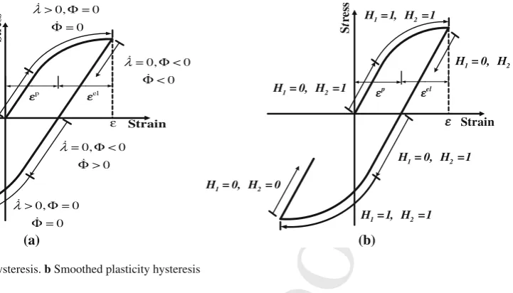
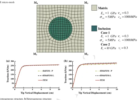
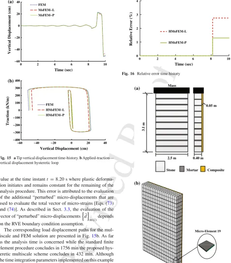
[image:5.595.157.518.55.261.2](b) Fig. 1 aClassical plasticity hysteresis.bSmoothed plasticity hysteresis
equal to zero, the material behaves elastically. The elastic 331
material behaviour corresponds to either small values of the 332
ratioΦ/Φ0or elastic unloading (in which caseΦ <˙ 0). On 333
the other hand, when bothH1=1 andH2=1 the material 334
yields. 335
Although rate forms are used herein for the sake of for-336
malism, an incremental procedure is implemented for their 337
solution, described in Sect.5.3. The continuum tangent mod-338
ulus of the model is readily derived from Eq. (20) as 339
[D]T =[D]([I]−H1H2[R]) (24) 340
In the case where a return-mapping scheme is implemented 341
for the solution of Eqs. (20) and (22), a consistent, smooth, 342
modulus can also be defined, following the procedure intro-343
duced in [50]. The implications of the selection of an appro-344
priate material modulus in conjunction with the solution pro-345
cedure implemented are also discussed in [56]. 346
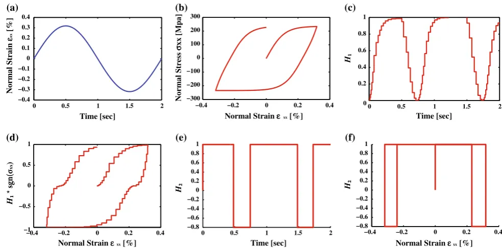
2.2 Test case 347
The behaviour of the smoothed Heaviside function is pre-348
sented through an illustrative example. A von-Mises no 349
hardening material is considered with the following mate-350
rial properties, namely E = 210 GPa, σy = 235 MPa,
351
N =2, β =0.1 andγ =0.9. One cycle of imposed strain 352
is applied and the corresponding time history is presented 353
in Fig.2a. The resulting stress–strain hysteresis loop is pre-354
sented in Fig.2b. Due to the small value of parameter N, 355
the transition from the elastic to the inelastic regime of the 356
response is smooth. Furthermore, the particular choice of 357
parametersβandγwithβ < γ results in a bulge hysteresis 358
loop, since the material stiffness at the beginning of unload-359
ing is slightly larger than the stiffness of elastic loading. 360
In Fig.2c, the time history of the smoothed Heaviside 361
function H1 is presented. The graph displays subsequent 362
regions of elastic loading, yielding and elastic unloading cor- 363 responding to the stress–strain hysteresis loop presented in 364 Fig.1b. In Fig.2d H1is multiplied by the sign of the corre- 365 sponding normal stress and plotted with respect to the strain. 366 Small values of imposed strain correspond to small values of 367 H1and the elastic response is retrieved in Fig.2b. Finally, in 368 Fig.2e and f the evolution of functionH2is presented with 369 respect to time and strain respectively. As predicted by the 370 model, in elastic loading it holds that H1=1 in both direc- 371 tions of strain. However, during unloading the value of H1 372 turns intoH1=β−γ = −0.8. As long as the valueH1is not 373 sufficiently small, the stiffness retrieved during unloading is 374 different than that of the elastic loading. 375 The smooth hysteretic model implemented in this work is 376 based on the Karray–Bouc model of hysteresis [16]. How- 377 ever, instead of relying on the assumptions of von-Mises yield 378 and linear kinematic hardening, the constitutive formulation 379 proposed herein accounts for any type of yield function and 380 kinematic hardening, within the framework of classical rate- 381 independent plasticity. The advantages of a Bouc–Wen type 382 model accounting for deformation dependent hardening were 383 recently highlighted in [47,60] where the linear kinematic 384 hardening coefficient of the Bouc–Wen model is substituted 385 by a continuous function derived from calibration of experi- 386
mental data. 387
2.3 The hysteretic finite element scheme 388
Substituting Eq. (1) into (2) the following relation is estab- 389
lished 390
{ ˙σ} =[D]
˙
εel=[D]{˙ε} −ε˙pl (25)
391
Comparing Eqs. (20) and (25) the following expression 392 for the evolution of the plastic strain component is readily 393
Revised
Proof
0 0.5 1 1.5 2
−0.4 −0.3 −0.2 −0.1 0 0.1 0.2 0.3 0.4
Time [sec]
Norm
a
l Str
a
in
ε
xx
[
%
]
(a)
−0.4 −0.2 0 0.2 0.4 −300
−200 −100 0 100 200 300
Normal Strain εxx [%]
Norm
a
l Stress
σ
xx [M
pa
]
(b)
0 0.5 1 1.5 2
0 0.2 0.4 0.6 0.8
1
Time [sec]
H
(c)
−0.4 −0.2 0 0.2 0.4 −1
−0.5 0 0.5 1
Normal Strain εxx [%]
H
xx
)
(d)
0 0.5 1 1.5 2
−0.8
−0.6 −0.4 −0.2 0 0.2 0.4 0.6 0.8
1
Time [sec]
H
(e)
−0.4 −0.2 0 0.2 0.4 −0.8
−0.6 −0.4 −0.2 0 0.2 0.4 0.6 0.8
1
Normal Strain εxx [%]
H
[image:6.595.49.541.54.297.2](f)
Fig. 2 aImposed strain.bStress–strain hysteresis loop.cTime history of smoothed Heaviside functionH1.dEvolution ofH1(normalized by the sign of the stress component) with respect to the imposed strain.eTime-history of Heaviside functionH2,fevolution ofH2with respect to the imposed strain
˙ εpl=
H1H2[R]{˙ε} (26)
395
where the interaction matrix [R] is defined in Eq. (21). The 396
discrete formulation is derived on the basis of the following 397
rate form of the principle of virtual displacements [57] 398
Ve
{ε}T{ ˙σ}
d Ve= {d}T
˙
f (27)
399
where{d}is the vector of nodal displacements over the finite 400
mesh,{f}is the corresponding vector of nodal forces and 401
Veis the finite volume of a single element. Only nodal loads
402
are considered herein for brevity however the evaluation of 403
body loads and surface tractions can be treated accordingly. 404
Substituting Eq. (25) into the variational principle (27) the 405
following relation is derived: 406
Ve {ε}T
[D]{˙ε}d Ve−
Ve {ε}T
[D]
˙ εpl
d Ve = {d}T
˙
f 407
(28) 408
The following interpolation scheme is considered for the con-409
tinuous displacement field{u} 410
{u} =[N]{d} (29)
411
with the accompanying strain-displacement compatibility 412
relation: 413
{ε} =[B]{d} (30)
414
where{d}is the vector of displacements at the finite element 415 nodes, [N] is the matrix of shape functions,{ε}is the vector 416 of strains evaluated at the nodes and [B]=∂[N] is the strain- 417 displacement matrix [18]. Substituting Eq. (30) into Eq. (28) 418 the following relation is derived: 419
Ve
[B]T [D] [B]d Ve
˙
d−
Ve
[B]T[D]
˙ εpl
d Ve =
˙
f 420
(31) 421
Next, a set of interpolation functions [Nσ] for the plastic part 422 of the strainεplis introduced, namely: 423
˙ εpl=
[Nσ]
˙ εpl
cq
(32) 424
where
εpl cq
is the vector of plastic strains measured at prop- 425 erly defined collocation points 426
εpl cq
= εpl cq
1
εpl cq
2
. . .εpl cq
ncqT
(33) 427
wherencqis the total number of collocation points within the 428 element. Substituting Eq. (32) in relation (31) the following 429 relation is finally derived: 430
kel d˙−
kh ε˙cqpl
Revised
Proof
wherekelis the elastic stiffness matrix of the element432
kel
=
Ve
[B]T[D] [B]d Ve (35)
433
andkhis the hysteretic matrix of the element. 434
kh
=
Ve
[B]T [D] [Nσ]d Ve (36)
435
Bothkelandkhare constant and inelasticity is controlled 436
at the collocation points through the accompanying plastic 437
strain evolution equations defined in Eq. (26). The latter is 438
based on the smooth plasticity model presented in Sect.2.1. 439
However, any type of plastic evolution law can be imple-440
mented. 441
The exact form of the interpolation matrix [Nσ] depends 442
on the element formulation and is also relevant to the stress 443
recovery procedure implemented within the finite element 444
formulation [56]. In this work the collocation points are 445
chosen to coincide with the Gauss quadrature points where 446
stresses are evaluated in standard FEM [65]. Furthermore, 447
smooth evolution equations of the form of relation (26) are 448
implemented. The classical formulation of classical plastic-449
ity however can be also used by considering the flow rule 450
defined in relation (3). 451
Equation (34) is the rate form of the equilibrium equa-452
tion. Considering zero initial conditions for brevity, rates are 453
dropped and the equilibrium equation of the hysteretic finite 454
element scheme assumes the following form 455
kel
{d} −
kh εcqpl
= {f} (37)
456
Equation (37) is supplemented by the set of nonlinear equa- 457 tions accounting for the evolution of the plastic part of the 458 deformation components defined at the collocation points. 459 These are the rates of the plastic strain vector defined in Eq. 460 (33) and assume the following form at the component level 461
˙ εpl
cq i q
=H1i qH2i q[R]i qε˙cq i q
, i q =1, . . . ,ncq (38) 462
Equations (37) and (38) form the governing equations of the 463 hysteretic finite element scheme. The latter is then used to 464 describe the micro-scale nonlinear behaviour of the multi- 465 scale scheme introduced in this work. 466
3 The enhanced multiscale finite element method 467
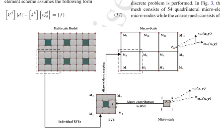
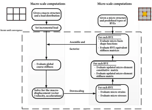
3.1 Overview 468
The EMsFEM is briefly presented in this section as a refer- 469 ence for subsequent derivations. In Fig.3the FEM computa- 470 tional model of a composite heterogeneous structure is pre- 471 sented. A 2D periodic structure, meshed with quadrilateral 472 plane stress elements is considered for brevity. However, the 473 numerical method presented in this work is also established 474 for the case of 3D meshes. The corresponding applications 475 are presented in Sect.6. Since EMsFEM is a computational 476 multiscale scheme, no requirements exist on the periodicity 477 of the underlying mesh [39]. 478 In the MsFEM the structure consists of two layers, namely 479 a fine-meshed layer up to the scale of the heterogeneities and 480 a coarse mesh of the macro-scale where the solution of the 481 discrete problem is performed. In Fig. 3, the fine element 482 mesh consists of 54 quadrilateral micro-elements and 70 483 micro-nodes while the coarse mesh consists of 6 quadrilateral 484
[image:7.595.42.486.437.695.2]Revised
Proof
macro-elements and 12 macro-nodes. Furthermore, twodis-485
placement fields are established corresponding to each level 486
of discretization. 487
Thus, in the fine mesh the displacement of a micro-488
material pointpis described by the micro-displacement vec-489
tor field 490
{dm} =
um(x,y) vm(x,y) T
491
Accordingly, the macro-displacement field is described by 492
the vector 493
{dM} =
uM(x,y) vM(x,y) T
494
In general, the subscriptm is used throughout this work to 495
denote a micro-measure while the capitalMis used to denote 496
a macro-measure of the indexed quantity. 497
Instead of implementing a one-step approach, i.e. solving 498
the fine meshed FEM model, a two-step solution procedure 499
is performed. In the first step, a mapping is numerically eval-500
uated that maps the fine mesh within each coarse-element 501
to the corresponding macro-nodes. Next, the solution proce-502
dure is performed in the coarse mesh. Finally, the fine-mesh 503
stress and strain history is retrieved by implementing the 504
inverse micro-mapping procedure onto the results obtained 505
on the coarse mesh. 506
3.2 Numerical evaluation of micro-scale basis functions 507
The numerical mapping is established by considering each 508
type of coarse element and its corresponding fine mesh as 509
a sub-structure. Considering groups of coarse-elements that 510
bare the same geometrical and mechanical properties these 511
coarse element types can be grouped into sets of represen-512
tative volume elements (RVE). In this work the term RVE 513
will be used to denote the coarse element together with its 514
underlying fine mesh structure as in [62]. For each RVE a 515
homogeneous equilibrium equation is established consider-516
ing specific boundary conditions. The solution of this equi-517
librium problem forms a vector of basis functions that maps 518
the displacement components of the fine mesh within the 519
element to the macro-nodes of the RVE. 520
In Fig.4, the RVE finite element mesh of the periodic com-521
posite structure (Fig.3) is presented. This mesh is assigned 522
a local nodal numbering since it is solved as an independent 523
structure. 524
EMsFEM is based on the assumption that the discrete 525
micro-displacements within the coarse element are interpo-526
lated at the macro-nodes using the following scheme: 527
um(xi,yi)=
nMacr o
j=1
Ni j x xuMj +
nMacr o
j=1
Ni j x yvMj 528
vm(xi,yi)=
nMacr o
j=1
Ni j x yuMj +
nMacr o
j=1
Ni j yyvMj (39) 529
Fig. 4 Finite element mesh of an RVE
Ni j x x =Nj x x(xi,yi) , Ni j yy =Nj yy(xi,yi) , 530 Ni j x y =Nj x y(xi,yi) , i =1, . . . ,nmi cr o 531
where um, vm are the horizontal and vertical components 532 of the micro-nodes, nmi cr o is the number of micro-nodes 533 within the coarse element,nMacr ois the number of macro- 534 nodes of the coarse element, (xi,yi)are the local coordi- 535 nates of the micro-nodes,uMj, vMj are the horizontal and 536 vertical displacement components of the macro-nodes and 537 Nj x x, Nj x y, Nj yyare the micro-basis functions. In MsFEM 538 as well as the interpolation techniques of the standard dis- 539 placement based finite element procedure [8] the interpolated 540 displacement fields are considered uncoupled. However in 541 EMsFEM the coupling terms Ni j x y are introduced that are 542 more consistent with the observation that a unit displacement 543 in the boundary of a deformable body may induce displace- 544 ments in both directions within the body. 545 It can be demonstrated [20,62] that a necessary and suf- 546 ficient condition for relations (39) to hold is that the micro- 547 basis functions adhere to the following property 548
nMacr o
i=1
Ni j x x =1
nMacr o
i=1
Ni j x y=0
nMacr o
i=1
Ni j yx=0
nMacr o
i=1
Ni j yy =1
, j =1, . . . ,nMacr o 549
(40) 550
Further details on the numerical evaluation of the micro-basis 551 functions are given in the Appendix section. 552 Considering the micro to macro-displacement mapping 553 introduced in relation (39), the following equation can be 554 established in the micro-elemental level 555
{d}m(i)=[N]m(i){d}M (41) 556
where {d}m(i) is the nodal displacement vector of theit h 557 micro-element, [N]m(i)contains the micro-basis shape func- 558 tions evaluated at the nodes of theit h micro-element while 559 {d}Mis the vector of nodal displacements of the correspond- 560 ing macro-nodes. For the case of micro-element #6 of the 561 coarse-element presented in Fig.4, the corresponding micro 562 and macro-displacement vectors assume the following form, 563
Revised
Proof
{d}m(6) =
um9vm9um10 vm10um14vm14 um13 vm13
T
565
(42) 566
and 567
{d}M =
uM1vM1uM2vM2uM6vM6uM5vM5
T
(43) 568
respectively. Variablesumi andvmiin Eq. (42) stand for the
569
horizontal and vertical displacement component of micro-570
nodei whileuM j andvM j in Eq. (43) are the
correspond-571
ing macro-displacement components of coarse node j. The 572
micro-basis shape function matrix is defined as: 573
[N]m(6) 574
=
⎡ ⎢ ⎢ ⎢ ⎢ ⎢ ⎢ ⎢ ⎢ ⎢ ⎢ ⎣
N9,1x x N9,1x y N10,1x x N10,1x y N14,1x x N14,1x y N13,1x x N13,1x y
N9,1x y N9,1yy N10,1x y N10,1yy N14,1x y N14,1yy N13,1x y N13,1yy
N9,2x x N9,2x y N10,2x x N10,2x y N14,2x x N14,2x y N13,2x x N13,2x y
N9,2x y N9,2yy N10,2x y N10,2yy N14,2x y N14,2yy N13,2x y N13,2yy
N9,3x x N9,3x y N10,3x x N10,3x y N14,3x x N14,3x y N13,3x x N13,3x y
N9,3x y N9,3yy N10,3x y N10,3yy N14,3x y N14,3yy N13,3x y N13,3yy
N9,4x x N9,4x y N10,4x x N10,4x y N14,4x x N14,4x y N13,4x x N13,4x y
N9,4x y N9,4yy N10,4x y N10,4yy N14,4x y N14,4yy N13,4x y N13,4yy ⎤ ⎥ ⎥ ⎥ ⎥ ⎥ ⎥ ⎥ ⎥ ⎥ ⎥ ⎦ 575
(44) 576
The(2nmi cr o×1)vector of nodal displacements of the
577
micro-mesh{d}m is evaluated as:
578
{d}m=[N]m{d}M (45)
579
where in this example 580
{d}m=
um1vm1um2vm2um3vm3. . .um16 vm16
T
581
(46) 582
and{d}M is defined in Eq. (43).
583
Matrix [N]m in Eq. (45) is a 32×8 matrix containing
584
the components of the micro-basis shape functions evaluated 585
at the nodal pointsxj,yj ,j = 1, . . . ,16 of the
micro-586
mesh. According to the property introduced in Eq. (40), each 587
column of [N]m corresponds to a deformed configuration of
588
the RVE where the corresponding macro-degree of freedom 589
is equal to unity and all of the remaining macro-degrees of 590
freedom are equal to zero. 591
Deriving micro-basis functions with these properties can 592
be accomplished by considering the following boundary 593
value problem 594
[K]RV E{d}m = {∅}
595
{d}S=
¯
d (47)
596
where [K]RV E is the stiffness matrix of the RVE,{d}Sis a
597
vector containing the nodal degrees of freedom defined at 598
the boundarySof the RVE andd¯is a vector of prescribed 599
displacements. The r.h.s vector{/0}in Eq. (47) stands for the 600
zero vector. 601
The RVE stiffness matrix [K]RV Eis formulated using the
602
standard finite element method [8]. Thus, [K]RV E is
assem-603
bled by evaluating the contribution of the individual stiffness 604
of each micro-element in the stiffness of the RVE, the latter 605 being considered as a stand-alone structure. In this work, the 606 direct stiffness method [65] is implemented for that purpose. 607 In the example case presented in Fig.4, the RVE consists of 608 16 nodes and 9 quadrilateral plane stress elements. Therefore, 609 the corresponding [K]RV E is a 32×32 matrix. 610 Each column of the shape function matrix [N]min Eq. (45) 611 corresponds to a displacement pattern derived from the solu- 612 tion of the linear system introduced in Eq. (47) for a specific 613 set of boundary conditions. Thus, for the example case pre- 614 sented in Fig.4, eight (8) different prescribed displacement 615 vectorsd¯need to be defined and the corresponding solu- 616 tions need to be performed. In this work, the solution of the 617 boundary value problem established in Eq. (47) is performed 618 using the Penalty method [9,23]. 619 The type of the boundary conditions implemented for the 620 evaluation of the micro-basis shape functions significantly 621 affects the accuracy of EMsFEM. Four different types of 622 boundary conditions are established in the literature namely 623 linear boundary conditions, periodic boundary conditions, 624 oscillatory boundary conditions with oversampling and peri- 625 odic boundary conditions with oversampling. In the first case, 626 the displacements along the boundaries of the coarse element 627 are considered to vary linearly. Periodic boundary conditions 628 are established by considering that the displacement compo- 629 nents of periodic nodes lying on the boundary of the coarse 630 element differ by a fixed quantity that varies linearly along 631 the boundary of the coarse element. The oscillatory bound- 632 ary condition method with oversampling considers a super- 633 element of the coarse element whose basis functions are eval- 634 uated using the linear boundary condition approach. Finally, 635 the periodic boundary conditions with oversampling com- 636 bine the oversampling technique with the periodic boundary 637 condition method, thus allowing for the implementation of 638 the latter in non-periodic RVE meshes [39,63]. 639 In this work, the cases of linear and periodic boundary 640 conditions are considered. An example on the application of 641 the periodic boundary conditions is described in the Appen- 642 dix, however further details on the procedure implemented 643 for the derivation of the micro-basis functions can be found 644
in [20,63]. 645
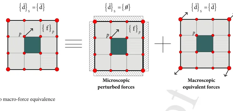
3.3 Macro equivalent micro-nodal forces 646
Revised
Proof
Fig. 5 Micro to macro-force equivalence
between the macro and the micro-scale [63], the following 656
relation is derived for the equivalent macro-loads 657
{F}M(i)=[N]mT(i){F}m(i) (48)
658
where{F}M(i) is the equivalent force vector of the
micro-659
nodal forces{F}m(i) of theit h micro-element. Since these
660
equivalent forces are derived in terms of an energy equiva-661
lence principle, compatibility within the fine mesh needs to 662
be enforced by calculating a set of “perturbed” micro-forces. 663
The micro-forces, acting on the micro-nodes will result in 664
the correct stress distribution within the fine mesh without 665
altering the displacement assumption along the boundary of 666
the coarse-element. 667
Therefore, an additive decomposition scheme is enforced 668
where the effect of a micro-force nodal vector{f}pacting
669
on a micro-nodepis decomposed into the effect of the same 670
force on the fine mesh but considering fixed boundaries and 671
the effect of the macro-equivalent forces on the coarse ele-672
ment (Fig.5). 673
The local effect of the “perturbed” micro-forces on the 674
micro-mesh is numerically evaluated from the solution of 675
the following equilibrium equation 676
[K]RV E
˜ d
m =
˜ F
m
677
˜ d
S=
¯
d (49)
678
where
˜ F
mis the vector of nodal “perturbed” micro-forces,
679
˜ d
mis the corresponding nodal displacement vector, while
680
˜ d
Sis the vector of imposed boundary conditions
¯
d. The 681
boundary conditions considered are similar to the boundary 682
conditions implemented for the evaluation of the micro to 683
macro mapping [Eq. (47)] [62,63] . 684
The evaluation of the “perturbed” micro-displacement 685
vector is crucial for the efficiency of the multiscale scheme 686
and will be further treated in Sect.5.2where the numerical 687
aspects of the proposed method are presented. Equivalently, 688
the actual stress field within the micro-element needs to be 689 evaluated taking into account the contribution of both the 690 micro-forces evaluated from the micro to macro-mapping 691
and the “perturbed” forces. 692
4 The hysteretic multiscale analysis scheme 693
4.1 Equilibrium in the fine scale 694
In this work the hysteretic finite element scheme defined by 695 Eqs. (37) and (38) is used to formulate the governing equa- 696 tions of the micro-scale. Thus, at the micro-scale the follow- 697
ing relations are defined 698
kel
m(i){d}m(i)−
kh
m(i)
εpl cq
m(i)= {f}m(i) (50)
699
and 700
˙ εpl
cq i q
m(i)=H i q
1 H
i q
2 [R]
i qε˙ cq
i q
m(i), i q=1, . . . ,ncq 701
(51) 702
where the index m(i)denotes the corresponding measure 703 of theit hmicro-element. Substituting Eq. (41) into Eq. (50) 704 and pre-multiplying with [N]mT(i) the following relation is 705
derived: 706
kel
M
m(i){d}M −
kh
M
m(i)
εpl cq
m(i)= {f} M
m(i) (52) 707
where 708
kel
M
m(i)=[N] T m(i)
kel
m(i)[N]m(i) (53) 709
[image:10.595.105.477.52.229.2]Revised
Proof
kh
M
m(i)=[N] T m(i)
kh
m(i) (54)
714
Finally,{f}mM(i)in Eq. (52) is the equivalent nodal force vec-715
tor of the micro-element mapped onto the macro-nodes of 716
the coarse element and is evaluated from Eq. (55) below 717
{f}Mm(i)=[N]Tm(i){f}m(i) (55)
718
Rearranging terms, Eq. (52) can be cast in the following form 719
kel
M
m(i){d}M = {f} M
m(i)− {fh}mM(i) (56)
720
where 721
{fh}mM(i) = −
kh
M
m(i)
εpl cq
m(i) (57)
722
can be considered as a nonlinear correction to the externally 723
applied load vector{f}mM(i). 724
Equation (52) is a multiscale equilibrium equation involv-725
ing the displacement vector{d}Mthat accounts for the nodal
726
displacements of the coarse-element nodes and the plastic 727
part of the strain tensor
εpl cq
m(i) that is evaluated at
col-728
location points within the micro-scale element mesh. Using 729
the micro-displacement to macro-displacement interpolation 730
relation [Eq. (41)] the micro-element state matrices, namely 731
the elastic stiffness matrix and the hysteretic matrix, defined 732
in Eqs. (35) and (36) respectively are mapped onto their mul-733
tiscale counterpartskelMm(i)andkhMm(i). 734
The derived multiscale elastic stiffness and hysteretic 735
matrices are constant and need only be evaluated once during 736
the analysis procedure. Therefore, the corresponding micro-737
basis functions introduced in relation (47) are also evaluated 738
once, thus significantly reducing the required computational 739
cost. 740
4.2 Micro to macro scale transition 741
Having established the micro-element equilibrium in Eq. (52) 742
in terms of macro-displacements using the micro-basis map-743
ping introduced in Eq. (41), a procedure is required to also 744
formulate the global structural equilibrium equations in terms 745
of macro-quantities. Denoting with a subscriptMthe corre-746
sponding macro-measures over the volumeV of the coarse 747
element, the Principle of Virtual Work is established at the 748
coarse scale as 749
VM {ε}T
M{σ}Md VM = {d}TM{f}M (58)
750
where{f}Mis the vector of nodal loads imposed at the coarse
751
element nodes. Equivalently to relation (34) the variational 752
principle of equation (58) gives rise to the following equation: 753
VM {ε}T
M{σ}Md VM =
Kel
M
C R(j){d}M
754
−Kh
M
C R(j) εpl cq M (59) 755
whereKelMC R(j),KhMC R(j)are the equivalent elastic stiff- 756 ness and hysteretic matrix of the jt hcoarse element respec- 757 tively while
εpl cq
M is the vector of plastic strains defined
758 at the collocation points. Within the multiscale finite ele- 759 ment framework, these quantities are not known a priori and 760 need to be expressed in terms of micro-scale measures, thus 761 accounting for the micro-scale effect upon the macro-scale 762 mesh. This is accomplished by postulating that the strain 763 energy of the coarse element is additively decomposed into 764 the contributions of each micro-element within the coarse- 765 element. Thus, the following relation is established: 766
V
{ε}T
M{σ}Md V = mel
i=1
Vm(i) {ε}T
m(i){σ}m(i)d V(i) (60) 767
where{ε}m(i),{σ}m(i)are the micro-strain and micro-stress 768 field defined over the volumeVm(i)of theithmicro-element. 769 Using relation (37), the following equation is established for 770 the r.h.s of equation (60) 771
mel
i=1
Vm(i) {ε}T
m(i){σ}m(i)d V(i) 772
=
mel
i=1
"
{d}mT(i)
kel
m(i){d}m(i)
773
− {d}miT
kh
m(i)
εpl cq
m(i) #
(61) 774
Substituting relation (45) into relation (61) gives rise to the 775
following expression 776
mel
i=1
Vmi {ε}T
m(i){σ}m(i)d Vi = {d}TM 777
·
mel
i=1
"
[N]TM(i)
kel
m(i)[N]M(i){d}M 778
−[N]TM(i)
kh
m(i)
εpl cq
m(i)
#
(62) 779
Substituting Eqs. (59) and (62) into Eq. (60), the following 780
expression is derived: 781
Kel
M
C R(j){d}M −
Kh
C R(j) εpl cq 782 = mel
i=1
kel
M
m(i){d}M − mel
i=1
kh
M
m(i)
εpl cq
Revised
Proof
Relation (63) holds for every compatible vector of nodaldis-784
placements{d}M as long as:
785
Kel
M
C R(j)= mel
i=1
kel
M
m(i) (64)
786
and 787
Kh
M
C R(j)
εpl cq
M =
mel
i=1
kh
M
m(i)
εpl cq
m(i) (65)
788
thus, substituting in relation (59) the following multiscale 789
equilibrium equation is derived for the coarse element: 790
Kel
M
C R(j){d}M = {f}M − {fh}M (66)
791
Vector{fh}M in Eq. (66) is the nonlinear correction to the
792
external force vector. This correction is evaluated by consid-793
ering the micro to macro mapping arising from the evolution 794
of the plastic strains within the micro-structure. 795
{fh}M = − mel
i=1
kh
M
m(i)
εpl cq
m(i)= mel
i=1
{fh}mM(i) (67)
796
where{fh}mM(i)has been defined in Eq. (57) while the plastic
797
strain vectors
εpl cq
m(i) are considered to evolve according
798
to relation (26). 799
Equations (66) and (67) are used to derive the equilibrium 800
equation at the structural level as will be described in the 801
next section. In analogy to the equilibrium equation of the 802
micro-element (mapped onto the coarse element) defined in 803
relation (56), the hysteretic force nodal load vector{fh}M is
804
the nonlinear correction to the external force vector{f}M at
805
the coarse element level. However, the evolution of{fh}M
806
is manifested through the evolution of the plastic deforma-807
tions at the micro-level and is therefore the link between the 808
inelastic processes occurring at the fine scale and the macro-809
scopically observed nonlinear structural behaviour. 810
The coarse element stiffness matrices are evaluated con-811
sidering only their individual micro-mesh properties. Thus, 812
they are independent and their evaluation can be performed 813
in parallel. 814
5 Solution procedure 815
5.1 Governing equations in the macro-scale 816
Considering the general case of a coarse mesh withndo fM
817
free macro-degrees of freedom and using Eq. (66), the global 818
equilibrium equations of the composite structure can be 819
established in the coarse mesh. In the dynamic case the fol-820
lowing equation is established: 821
[M]C R
¨
UM +[C]C R
˙
UM 822
+Kel
C R{U}M = {F}M − {Fh}M (68) 823
where [M]C R,[C]C R,
KelC Rare the(ndo fM×ndo fM) 824 macro-scale mass, viscous damping and stiffness matrix 825 respectively, evaluated at the coarse mesh. 826 The formulation of the mass matrix, defined at the coarse 827 mesh, is established on the grounds of the micro-basis shape 828 functions presented in Sect.3. This leads to a multi-scale 829 consistent mass matrix formulation where the derived mass 830 matrix is non-diagonal. Well-known mass diagonalization 831 techniques can then be performed to derive an equivalent 832 lumped mass matrix [18]. However, the implications of such 833 approaches are beyond the scope of this work. Similarly, the 834 viscous damping can be of either the classical or non-classical 835
type [17]. 836
The global stiffness matrix of the structure, defined at 837 the coarse mesh, is formulated through the direct stiffness 838 method from the contributions of the coarse elements equiv- 839 alent stiffness matricesKelMC R(j)[Eq. (64)]. Accordingly, 840 the(ndo fM×1)vector{U}M consists of the nodal macro- 841
displacements. 842
The external load vector {F}M and the hysteretic load 843 vector{Fh}M are assembled considering the equilibrium of 844 the corresponding elemental contributions{f}M and{fh}M, 845 defined in Eqs. (58) and (67) respectively, at coarse nodal 846
points. 847
Equation (68) is supplemented by the evolution equations 848 of the micro-plastic strain components defined at the colloca- 849 tion points within the micro-elements. These equations can 850 be established in the following form: 851
˙ Ecqpl
m =[G]
˙
Ecq
m (69) 852
where the vector 853
˙ Ecqpl
m = ε˙
pl cq
m(1)
˙ εpl
cq
m(2). . .
˙ εpl
cq
m(mel)
T
(70) 854
holds the plastic strain components evaluated at the colloca- 855 tion points of each micro-element and 856
˙
Ecq
m = ε˙cq
m(1)
˙ εcq
m(2) . . .
˙ εcq
m(mel)
T
(71) 857
Revised
Proof
[G]=⎡ ⎢ ⎢ ⎢ ⎢ ⎢ ⎢ ⎢ ⎢ ⎢ ⎢ ⎢ ⎢ ⎣ ⎡ ⎢ ⎣
[g1] ...
gncq
⎤ ⎥ ⎦
(1) ...⎡
⎢ ⎣
[g1] ...
gncq
⎤ ⎥ ⎦
(mel)
⎤ ⎥ ⎥ ⎥ ⎥ ⎥ ⎥ ⎥ ⎥ ⎥ ⎥ ⎥ ⎥ ⎦ 862 (72) 863
wheregi q
,i q=1, . . . ,ncqare 6×6 sub-matrices defined
864 as 865
gi q(i) =H1i qm(i)H2i qm(i)[R]i qm(i)
866
andncqis the total number of collocation points within each
867
micro-element. 868
Equations (69) are independent and thus can be solved 869
in the micro-element level resulting in an implicitly paral-870
lel scheme. Both relations (69) and (72) depend on the cur-871
rent micro-stress state within each micro-element and conse-872
quently on the micro-strain and micro-displacement distrib-873
ution. Thus, a procedure needs to be established that down-874
scales the macro-displacements{U}Mevaluated at the coarse
875
mesh to the micro-displacements of the micro-nodes within 876
the fine mesh. 877
5.2 Downscale computations 878
Considering that the value of the coarse mesh displace-879
ments{U}M is known, the interpolation scheme introduced
880
in relation (39) can be used to derive the micro-displacement 881
components within each coarse element. Extracting the 882
nodal macro-displacements{d}M of a macro-element from
883
{U}M the corresponding micro-displacement vector of the
884
it h micro-element {d}m(i) is derived through relation (41)
885
that is re-written here for brevity 886
{d}m(i)=[N]m(i){d}M (73)
887
However, this micro-displacement vector only contains infor-888
mation derived from the macro to micro-displacement map-889
ping and does not take into account the local effect of the 890
micro-displacement on the neighbouring micro-nodes, as 891
discussed in Sect.3.3. Therefore, the actual displacement 892
vectord¯m(i)that is compatible with the strain field within 893
the micro-element is evaluated as 894
¯
dm(i)= {d}m(i)+
˜ d
m(i) (74)
895 where ˜ d
m(i)is evaluated from relation (49). The total strain
896
vector at the collocation points is then evaluated by using the 897
strain-displacement relation defined in Eq. (30) 898
εcq i q
m(i)=[B] i q m(i)
¯
dm(i), i q=1, . . . ,ncq (75)
899
wherencqis the number of collocation points within the ele- 900 ment and [B]i qm(i)is the strain-displacement matrix evaluated 901 at each collocation pointi q. The rate of total strains is derived 902
accordingly through 903
˙ εcq
i q
m(i) =[B] i q m(i)
˙¯ d
m(i), i q=1, . . . ,ncq (76)
904
The total stresses at the collocation points are evaluated by 905 integrating Eqs. (25) and (22) defined at the micro-scale as 906
˙ σcq
i q
m(i)=[D]m(i) "
˙ εcq
i q m(i)−
˙ εpl
cq i q
m(i) # (77) 907 and 908 ˙ ηcq i q
m(i) 909
=H1i qm(i)H2i qm(i)G
{η}i q m(i), Φ
i q m(i) R˜
i q
m(i)
˙ εcq
i q
m(i) 910
(78) 911
respectively. Equations (77) and (78) are supplemented by 912 the following set of evolution equations for the plastic strain 913
˙ εpl
cq i q
m(i)=H i q
1m(i)H i q
2m(i)[R] i q m(i)
˙ εcq
i q
m(i) (79) 914
Since the current micro-stress state is required to evaluate 915 the Heaviside functions H1i qm(i), H2i qm(i) [Eqs. (17) and (18) 916 respectively] and the interaction matrix [R]m(i)[Eq. (21)] an 917 iterative procedure is required at the micro-element level. 918
5.3 Newton iterative scheme 919
In this section, the nonlinear static analysis procedure imple- 920 mented is presented for clarity, while the dynamic case is 921 treated accordingly using the Newmark average acceleration 922 method to integrate the equations of motion [17]. 923 Dropping the inertia and viscous damping terms from Eq. 924 (68) the following equation is derived: 925
Kel
C R{d} = {F}M− {Fh}M (80)
926
Considering an iterative Newton–Raphson incremental 927 scheme the following equation is established 928
Kel
C R j
i {d} = j
i {P} −
j
i{Fh}M (81) 929
where j stands for the current iteration within the current 930 loading stepi,ij{P}is the current externally applied force 931 increment that at the beginning of the load increment is eval- 932
uated as: 933
0
i {P} =i
Pext−i−1
Pext (82) 934