Generalized Shift Splitting Preconditioner for Saddle Point Problems with Block Three by Three Structure

(1)

ISSN Online: 2333-9721 ISSN Print: 2333-9705

DOI: 10.4236/oalib.1105968 Dec. 25, 2019 1 Open Access Library Journal

Generalized Shift-Splitting Preconditioner

for Saddle Point Problems with Block

Three-by-Three Structure

Linna Wang, Ke Zhang

*

Department of Mathematics, Shanghai Maritime University, Shanghai, China

Abstract

We propose a generalized shift-splitting iteration method for saddle point problems with block three-by-three structure. As a new iteration method, the method converges to the unique solution of the saddle point problem uncon-ditionally. When exploited as a preconditioner, the spectral distribution of the preconditioned matrix is investigated. Numerical experiments show that the new variant is efficient in speeding up GMRES for solving the block three-by-three saddle point problem.

Subject Areas

Numerical Mathematics

Keywords

Saddle Point Problem, Generalized Shift-Splitting, Krylov Subspace, GMRES

1. Introduction

We consider the saddle point problems with the following block three-by-three structure

T T 0

0 or ,

0 0

A B x f

B C y g u b

C z h

 _{    }  _{    }

− − = =

 _{    }  _{    }_{   }

 

 (1)

where _A_∈_n n× _{is a symmetric positive definite matrix,} _B_∈_m n× _and s m

C_∈_× _{are matrices of full row rank,} _f _∈_n_, _g_∈_m_and _h_∈_s_{are given}

vectors. The linear system of equations (1) has many practical applications in How to cite this paper: Wang, L.N. and

Zhang, K. (2019) Generalized Shift-Split- ting Preconditioner for Saddle Point Pro- blems with Block Three-by-Three Structure. Open Access Library Journal, 6: e5968.

https://doi.org/10.4236/oalib.1105968

Received: November 29, 2019 Accepted: December 22, 2019 Published: December 25, 2019

This work is licensed under the Creative Commons Attribution International License (CC BY 4.0).

http://creativecommons.org/licenses/by/4.0/

(2)

DOI: 10.4236/oalib.1105968 2 Open Access Library Journal scientific computing and engineering fields, including the constrained quadratic optimization problem, the constrained least squares problem and the computa-tional fluid dynamics [1].

In practice, the coefficient matrix  in (1) is generally sparse and of large size. Therefore, iterative methods are usually preferred for their low memory requirement per iteration. Among these candidates, the Uzawa-type methods [2], the matrix splitting methods [3] and the Krylov subspace methods [4] have re-ceived much attention during the past decades. For instance, the Uzawa method [2] is a classical approach which is known for its low computational overhead and easy implementation. To improve the numerical performance, some Uza-wa-type variants have been proposed recently which include the inexact Uzawa [5] [6] [7], Uzawa-SOR [8] and Uzawa-PSS [9], etc. The other way for solving the saddle point problems is to exploit the matrix splitting. By using the Hermi-tian and skew-HermiHermi-tian splitting (HSS), Bai et al. [3] propose the HSS iteration method. Following this reasoning, some efficient variants such as the accelerated Hermitian and skew-Hermitian splitting (AHSS) [10], the modified Hermitian and skew-Hermitian splitting (MHSS) [11] and the relaxed Hermitian and skew- Hermitian splitting (RHSS) [12] have been proposed henceforth. Recently, the sophisticated Krylov subspace methods have been used to solve the saddle point problems. Due to the structure of the saddle point matrices, however, a slow convergence or even stagnation is often witnessed during the actual computation. Such drawback can be alleviated by employing an appropriate preconditioner. In the context of saddle point problems, many efficient preconditioners, to name just a few, the block diagonal preconditioners, the constrained preconditioners, the HSS-based preconditioners, have been developed; see [13] [14] [15] [16] and the more recent monograph [17] for detail.

In [18], Bai et al. propose a class of shift-splitting iteration method for solving non-Hermitian positive definite linear system Au b= . It can be recast in the following way. Suppose that _A_∈_n n× _{is a non-Hermitian positive definite}

ma-trix. Then the shift-splitting of the coefficient matrix A is given by

( )

1

(

)

1

(

)

,

2 2

A M= α −N α = αI A+ − αI A−

which leads naturally to the shift-splitting iteration scheme

( ) ( )

( )

1 1 1 _, _0,1,2,

k k

u + ₌M−

α

N

α

u ₊M−

α

b k₌

(3)

ge-DOI: 10.4236/oalib.1105968 3 Open Access Library Journal neralized saddle point problems and propose a modified generalized shift-splitting preconditioner [21].

By taking into account the special structure of (1), Cao [22] proposes shift- splitting preconditioners for solving (1). Motivated by [20] and [22], we devise a new generalized shift-splitting (GSS) iteration scheme for the structured linear system (1). A corresponding GSS preconditioner is induced to accelerate the convergence of GMRES. Theoretical results on the convergence of GSS iteration method and the eigenvalue distribution of the preconditioned matrix are also given.

The organization of this paper is as follows. In Section 2, we introduce the ge-neralized shift-splitting iteration method for solving the block three-by-three saddle point problem and look into its convergence property. In Section 3, we obtain a GSS preconditioner derived from the GSS iteration and analyze the spectrum of the preconditioned matrix. In Section 4, some numerical experi-ments are carried out to illustrate the effectiveness of GSS by comparing it with other shift-splitting preconditioners given in [22]. Finally, some conclusions are given in Section 5.

2. Generalized Shift-Splitting Iteration Method and Its

Convergence

The proposed generalized shift-splitting (GSS) iteration is based on the work of [22]. Therefore, it is reasonable for us to recap briefly the shift splitting used in [22] before introducing the new iteration method in this section.

In its simplest form, the shift splitting (SS) of the coefficient matrix  in (1) goes as follows

(

)

(

)

T T

1 1

2 2

0 0

1 1 _,

2 2

0 0

I I

I A B I A B

B I C B I C

C I C I

α α

= + − −

 +   − − 

   

= _ − − _− _ _

   ₋ 

   

  

(2)

where I is the identity matrix with conforming size. The parameter

α

_{in (2) is} used to monitor the convergence of the SS iteration method and hence the spec-trum of the preconditioned matrix. In other words,

α

_{plays the same role in} adjusting the two block diagonal matrices in (2), i.e.,

( ) ( )

T

and 0 . 0

m n m n s s

A B B

+ × + ×

 

∈ ∈

₋ 

    (3)

(4)

DOI: 10.4236/oalib.1105968 4 Open Access Library Journal splitting

(

)

(

)

(

)

(

)

T T T T 1 1 , , 2 2 0 0

1 1 _.

2 ₀ 2 ₀

M N

I A B I A B

B I C B I C

C I C I

α β α β

α α

β β

= − = Ω + − Ω −

 +   − −      = _ − − _− _ _    ₋         (4)

Here α >0_, β >0 and

I I I α α β    

Ω =  

 

 

. Then it is trivial to find that

the generalized shift-splitting (4) reduces to the shift-splitting (2) if

α β

= _.

Using the splitting (4), we obtain the following stationary iteration

1 _,

k k

GSS

u + _{= Γ} u ₊c ₍₅₎

where 1

(

_,

) (

_,

)

GSS M−

α β

N

α β

Γ = , _{c M}₌ −1

(

_{α β}

_,

)

_b_and _k₌_0,1,_{. To put it} another way, the generalized shift-splitting method (GSS) for the block three-by- three saddle point problem (1) that can be stated as follows. Given an initial vector _u0_{, compute}

T T

T 1 T

0 0

1 1

2 2

0 0

k k

I A B I A B f

B I C u B I C u g

C I C I h

α α α α β β +  +   − −     ₋ ₋  ₌   ₊           −   _{ }     (6)

until _uk_{converges, where} _k₌_0,1,_.

It is known that the GSS iteration method (5) enjoys the unconditional con-vergence if the spectral radius of the iteration matrix ΓGSS is less than 1. The

following results are adapted from [22] and [23] which are instrumental in prov-ing such sound convergence property.

Lemma 1. Suppose that _A_∈_n n× _{is a symmetric positive definite matrix}_, m n

B_∈_ × _and _C_∈_s m× _{are of full row rank}_._Let _λ_{be an eigenvalue of the}

saddle point matrix , then

( )

0.

Re λ >

Proof. The proof can be found in ([22], Lemma 2.2).

Lemma 2. Let _W_∈_n n× _{be a non-Hermitian positive semidefinite matrix}

and _{E W}

(

_,_δ

) (

_δ_{I W}

) (

−1 _δ_{I W}

)

= + − be the extrapolated Cayley transform with

0

δ > _._Then

1) the spectral radius of E W

(

,δ

)

_{is bounded by 1,}_i_._e_., ρ

(

E W

(

,δ ≤

)

1; 2) ρ

(

E W

(

,δ =

)

1 if and only if the matrix W has a (reducing) eigenvalue of the form ιξ with ξ ∈ and

ι

_{the imaginary unit.}

Proof. See ([23], Theorem 2.1) for detail.

The following theorem on the convergence of GSS iteration method comes out as a result of Lemma 1 and Lemma 2.

Theorem 1. Suppose that _A_∈_n n× _{is a symmetric positive definite matrix}_, m n

B_∈_ × _and _C_∈_s m× _{are matrices of full row rank}_._Let _{α >}₀_and _{β >}₀_.

(5)

DOI: 10.4236/oalib.1105968 5 Open Access Library Journal

(

GSS

)

1,

ρ Γ <

i.e., the GSS iteration method converges to the unique solution of (1) uncondi-tionally.

Proof. By (4) and (5), we rewrite the iteration matrix ΓGSS as

(

) (

1

)

1₂ 1₂ 1₂ 1 ₂1 ₂1 1₂

.

GSS I I

−

− − − − −

−    

Γ = Ω + Ω − = Ω _ + Ω Ω  _{ } − Ω Ω _Ω

   

   

Let _ˆ_{= Ω}−12__Ω−12_{. It is easy to see that}

GSS

Γ _{is similar to the matrix}

(

_ˆ

) (

1 _ˆ

)

ˆ_GSS _I − _I

Γ = + − . Therefore, it suffices to prove

ρ

( )

ΓˆGSS <1. By the construction of _ˆ _{= Ω}−12__Ω−12_{, we have}

( )

1 1 T 2 2 T

1 1 T

1

1 ₂ T

1 2 0 ˆ ₀ 0 0 0 0 . 0 0

I A B I

I B C I

I C I

A B B C C α α α α β β α α α αβ αβ − − − − − − −             =_ _ _− − __ _                  = −_ − _       

Since

α

_and

β

are positive, then _α−1_A_{is a symmetric positive definite} matrix, _α−1_B_and

( )

_αβ −1₂_C

are matrices of full row rank. Thus ˆ is a nonsymmetric positive semi-definite matrix. Moreover, it follows from Lemma 1 that Re

( )

λ

( )

_ˆ >0_{. Therefore, it can be deduced from Lemma 2 that}

( )

ˆ_GSS ₁

ρ

Γ ≤ _{. The equality}

ρ

( )

ΓˆGSS =1 holds if and only if ˆ has a (reducing) eigenvalue of the form

ιξ

, which is impossible because Re

( )

λ

( )

_ˆ >0_{. It turns} out that

ρ

( )

ΓˆGSS <1. As a result, ρ

(

ΓGSS

)

<1 which completes the proof.

3. GSS Preconditioner and Its Properties

Though the GSS iteration method is proved to converge unconditionally, its convergence can be rather slow when compared with the involved Krylov sub-space methods [24]. In the context of linear system solvers, it is more interesting to exploit the generalized shift-splitting as a preconditioner to accelerate the Krylov subspace methods like GMRES.

In this section, we present the following generalized shift-splitting precondi-tioner (GSS) T T 0 1 _. 2 ₀ GSS

I A B

B I C

C I α α β  +    = _ − − _    

 (7)

When applying a preconditioner, the convergence of the preconditioned li-near system is closely related with the eigenvalue distribution. The following finding shows that the eigenvalues of GSS-preconditioned matrix 1

GSS−

(6)

DOI: 10.4236/oalib.1105968 6 Open Access Library Journal right preconditioning here such that the residual of the original saddle point problem is the same as that of its right-preconditioned counterpart.

Theorem 2. Suppose that _A_∈_n n× _{is a symmetric positive definite matrix}_, m n

B_∈_ × _and _C_∈ s m×

 are matrices of full row rank. Let θ be an eigenvalue of 1

GSS−

 , then

1− <θ 1. Proof. Since the preconditioned matrix 1

GSS−

 is similar to 1

GSS−

 , then it is only necessary to investigate the spectrum of 1

GSS−

 . Since GSS =M

(

α β,

)

, then it follows from (4) that

(

)

(

)

(

)

(

)

(

)

(

)

1 1 1 , , , , , . GSS GSS GSS M N

M M N

I

α β α β α β α β α β

− −

−

= −

= − Γ

  

From Theorem 1, we know that 1− <θ 1_{, where}θ_{is an eigenvalue of}

1

GSS−

 .

Before ending this section, we give some implementation details when apply-ing the GSS preconditioner. In actual computations, a matrix-vector product

1

GSS− r

 is often needed which can be solved from the linear system GSSz r= .

Note that the preconditioner GSS can be decomposed as

1 T T T 1 T T T 1 T 1 ₀

1 ₀ 1

2

0 0

1 ₀ ₀

1

0 0

1 _{0 .}

1 0

GSS

I B I C C

I C

I

I A B I C C B

I C C

I

I C C B I

C I α β β α α β α β β α β β − − −  _ _  +  _ _          = −            _ _  + + +  _ _          ⋅ +                     ⋅ −_ _ + _ _            (8)

Let T T T T

1 , ,2 3

r_{= }r r r _ _and T T T T 1, ,2 3

z_{= }z z z _ _{, where}_{r z}₁, ₁_∈_n_,

2, 2 m

r z ∈

and r z3, 3∈s. By using the decomposition (8), we obtain the following

sub-routine for solving 1

GSS

z₌_− r_.

1) Solve w1 from αI _β1C C wT 1 2r2 _β2C rT 3

 

+ = +

 

(7)

DOI: 10.4236/oalib.1105968 7 Open Access Library Journal 2) Solve z1 from

1

T T T

1 1 1

1 ₂

I A B I C C B z r B w

α α β −  _ _   + + _ + _  = −  _ _    ;

3) Solve w2 from αI _β1C C wT 2 Bz1

 ₊  ₌

 

  ;

4) Update z2 =w w1+ 2; 5) Update z3=_β1 2

(

r Cz3− 2

)

.

In computing 1

GSS− r

 , the computational overhead by GSS is the same as that by SS [22]. As indicated in the numerical examples, however, an appropriate choice of

(

α β,

)

generally yields better numerical performance (concerning CPU time and iteration steps) than using a single parameter

α

_{(as in SS). In} this sense, the GSS can be regarded as a more promising variant than its prede-cessor SS.

4. Numerical Experiments

In this section, we give some numerical experiments to illustrate the effective-ness of the new preconditioner GSS in terms of the number of iteration steps (iter), CPU time in seconds (time) and the relative residual norm (res). For completeness, we display both the number of restarts and the number of inner steps in the last restart; see, for instance, Table 3. The unconditioned GMRES(k), the shift-spliting-preconditioned GMRES(k) (SS) [22] and the relaxed shift- splitting-preconditioned GMRES(k) (RSS) [22] are employed for comparison, where k is the restarting frequency. In what follows, the right preconditioning is used for SS, RSS and GSS, the reason of which is given in Section 3. We set the restarting frequency k to be 5 and the initial guess _u0_{to be the zero vector.} The right-hand side vector b in (1) is given by 10⋅rand m n s

(

+ + ,1

)

. All

algo-rithms mentioned above terminate if 6

2

2 10

i

b₋_u b _< − _{within 1500}

res-tarts, where _ui_{is the}_i_{th iterate. Numerical experiments are carried out on a}

laptop using MATLAB 2014b with Intel Core (8G RAM) under Windows 10 system.

The testing problem is adapted from [25]. It is a block three-by-three saddle point problem with A, B and C of the following structure

[

]

2 2 2 2 2 2 2 2 2 0 , 0 , , p p p p p p

I T T I A

I T T I

B I F F I

C E F

× × × ⊗ + ⊗   =_ _∈ ⊗ + ⊗   = ⊗ ⊗ ∈ = ⊗ ∈

where _T 1 tridiag 1,2, 1₂

(

)

p p

h

×

= ⋅ − − ∈_ _, _F 1 tridiag 0,1, 1

(

)

p p

h

×

= ⋅ − ∈_ _,

(

2

)

diag 1, 1, , 1

E= p+ p − +p with ⊗_{being the Kronecker product and}

1 1 h

p

=

(8)

4.1. Choice of the Parameter Pair

(

α β

,

)

As mentioned in Section 2, the main motivation for embracing an extra para-meter

β

in GSS is to strike a balance in controlling the sub-matrices in (3). A proper choice of

α

and

β

will make the GSS preconditioner more appealing. As shown in (7), the GSS preconditioner GSS becomes closer to (half of) the

saddle point matrix  as

α

and

β

decrease. This implies that the choice 0

α β= = seems to be the optimal one. However, we do not suggest using ex-tremely small values of

α

_and

β

for numerical concerns. Instead, we use the experimental (optimal) values of

α

_and

β

in the following experiments.

To this end, we first tabulate the CPU time of the GSS preconditioner with varying

α

_and

β

for p=16 and p=32 in Table 1 and Table 2, respec-tively. The parameter pair

(

α β,

) (

= 0.01,0.001

)

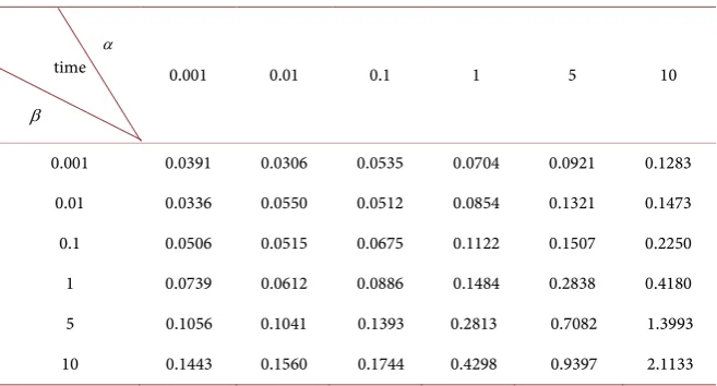
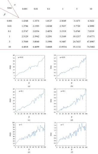
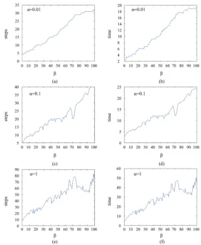
_{yields the shortest CPU time in} both tables. To further verify this finding, we carry out more experiments in Fig-ure 1 and Figure 2 by depicting the number of total iteration steps1_{and CPU time} of GSS with varying

β

when

α

_{is chosen to be 0.01, 0.1 and 1, respectively.} Some remarks are in order. Loosely speaking, for a fixed value of

α

_{, the number} of total iteration steps and CPU time increase as

β

goes up although there are some zigzags; see Figure 1 and Figure 2. Moreover, a similar pattern is also ob-served for

β

when the value of

β

is fixed while

α

varies; for instance, when

50

β

= _{, the total iteration steps increase as}

α

_{changes from 0.01 to 1, which} reads readily by comparing the subplots (a), (c) and (e) in Figure 1. This justifies our choice of using

(

α β,

) (

= 0.01,0.001

)

as the experimental optimal value.

[image:8.595.210.539.488.665.2]

Based on the above experiments, we use

(

α β,

) (

= 0.01,0.001

)

as the expe-rimental optimal choice for

α

and

β

in GSS. As for the optimal value of

α

Table 1. CPU time of the GSS preconditioner with different values of α and β

(p=16_). α

time

β

0.001 0.01 0.1 1 5 10

0.001 0.0391 0.0306 0.0535 0.0704 0.0921 0.1283 0.01 0.0336 0.0550 0.0512 0.0854 0.1321 0.1473 0.1 0.0506 0.0515 0.0675 0.1122 0.1507 0.2250 1 0.0739 0.0612 0.0886 0.1484 0.2838 0.4180 5 0.1056 0.1041 0.1393 0.2813 0.7082 1.3993 10 0.1443 0.1560 0.1744 0.4298 0.9397 2.1133

1_{By “total iteration steps”, we mean the total number of matrix-vector products associated with}

1

GSS −

(9)

DOI: 10.4236/oalib.1105968 9 Open Access Library Journal in SS and RSS, we follow the choice α =0.01_{used in}_[22]_{and regard it as the} empirical optimal value.

4.2. Comparison with Other SS-Type Methods

[image:9.595.211.539.180.693.2]

In this subsection, we compare the numerical performance of GSS with SS and

Table 2. CPU time of the GSS preconditioner with different values of α and β (p=32).

α time

β

0.001 0.01 0.1 1 5 10

0.001 1.4348 1.3374 1.8127 2.5649 3.1475 4.3422 0.01 1.3786 2.1595 1.8248 2.7657 3.7720 4.5090 0.1 2.3747 2.0354 2.4876 3.1519 5.4760 7.0319 1 2.5129 2.5942 3.2291 5.2169 10.1217 15.6771 5 3.7049 3.8040 5.1990 9.5487 24.7657 47.8987 10 4.4818 4.4699 5.6668 13.9554 35.1132 74.5482

(10)

[image:10.595.225.518.69.426.2]

Figure 2. Total iteration steps (left) and CPU time (right) of the GSS preconditioner for different values of α and β (p=32).

RSS regarding CPU time and iteration steps. It should be noted that all sub-linear equations involved in computing matrix-vector product _−1_r_{are solved by} direct methods.

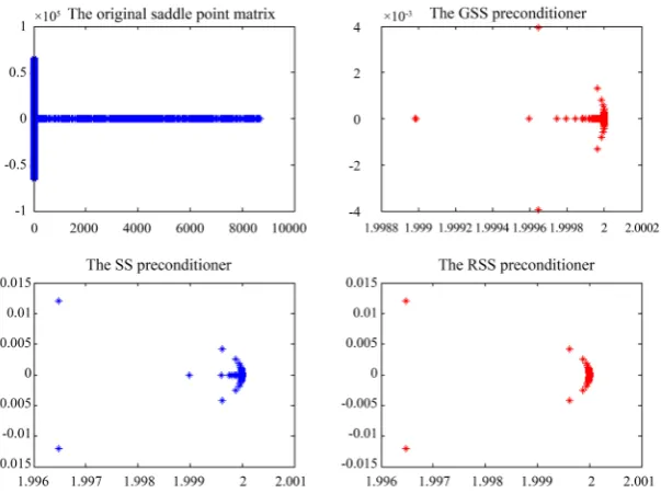
It is known that the spectrum imposes a great effect on the convergence of the preconditioned linear system. To begin with the discussion, we plot respectively the spectral distributions of the original saddle point matrix , the GSS-preconditioned matrix 1

GSS−

 , the SS-preconditioned matrix 1

SS−

 , and the RSS-preconditioned matrix 1

RSS−

(11)

[image:11.595.224.526.70.295.2]

Figure 3. Eigenvalue distributions of the unpreconditioned saddle point matrix and of three SS-type preconditioned matrices (p=32).

Table 3. Numerical results for three preconditioned GMRES methods with different grid sizes.

SS RSS GSS

size iter time res iter time res iter time res

16

p= 1(3) 0.0744 9.3431e−09 1(3) 0.0651 5.1792e−09 1(2) 0.0415 4.5483e−07

32

p= 1(3) 1.9894 8.5844e−09 1(3) 1.8084 4.4832e−09 1(2) 1.2381 3.4408e−07

48

p= 1(3) 16.5567 7.8697e−09 1(3) 16.2467 2.7591e−09 1(2) 10.9178 3.1121e−07

64

p= 1(3) 88.9495 7.6631e−09 1(3) 84.8754 2.641e−09 1(2) 57.3213 2.7896e−07

even if the problem size ₄_p2_{soars. Fortunately, this desirable property has also}

been carried over to GSS. Furthermore, GSS outperforms SS and RSS in that it requires the shortest CPU time and the least number of iteration steps in all test problems, as observed in Table 3. In light of this, we conclude that GSS is a competitive shift-splitting variant for solving the structured saddle point prob-lem (1).

5. Conclusion

[image:11.595.210.538.368.468.2]

(12)

DOI: 10.4236/oalib.1105968 12 Open Access Library Journal convergence of GMRES. It is proved that the preconditioned matrix using the new preconditioner has a well-clustered spectrum which is verified by the nu-merical examples. Future works include finding the theoretically optimal choice of the parameters in the new scheme and develop other efficient shift-splitting preconditioners.

Acknowledgements

This work is supported by the National Natural Science Foundation (grant number: 11601323) and the Key Discipline Fund (2018) of College of Arts and Sciences in Shanghai Maritime University. The authors would like to thank the referees for their constructive suggestions.

Conflicts of Interest

The authors declare no conflicts of interest regarding the publication of this pa-per.

References

[1] Benzi, M., Golub, G.H. and Liesen, J. (2005) Numerical Solution of Saddle Point Problems. Acta Numerica, 14, 1-137.https://doi.org/10.1017/S0962492904000212 [2] Arrow, K.J., Hurwicz, L. and Uzawa, H. (1958) Studies in Nonlinear Programming.

Stanford University Press,Redwood City, CA.

[3] Bai, Z.-Z., Golub, G.H. and Ng, M.K. (2003) Hermitian and Skew-Hermitian Split-ting Methods for Non-Hermitian Positive Definite Linear Systems. SIAM Journal on Matrix Analysis and Applications, 24, 603-626.

https://doi.org/10.1137/S0895479801395458

[4] Bai, Z.-Z. (2015) Motivations and Realizations of Krylov Subspace Methods for Large Sparse Linear Systems. Journal of Computational and Applied Mathematics, 283, 71-78. https://doi.org/10.1016/j.cam.2015.01.025

[5] Bramble, J.H., Pasciak, J.E. and Vassilev, A.T. (1997) Analysis of the Inexact Uzawa Algorithm for Saddle Point Problems. SIAM Journal on Numerical Analysis, 34, 1072-1092. https://doi.org/10.1137/S0036142994273343

[6] Cao, Z.-H. (2003) Fast Uzawa Algorithm for Generalized Saddle Point Problems. Applied Numerical Mathematics, 46, 157-171.

https://doi.org/10.1016/S0168-9274(03)00023-0

[7] Bai, Z.-Z. and Wang, Z.-Q. (2008) On Parameterized Inexact Uzawa Methods for Generalized Saddle Point Problems. Linear Algebra and Its Applications, 428, 2900- 2932. https://doi.org/10.1016/j.laa.2008.01.018

[8] Zhang, J. and Shang, J. (2010) A Class of Uzawa-SOR Methods for Saddle Point Problems. Applied Mathematics and Computation, 216, 2163-2168.

https://doi.org/10.1016/j.amc.2010.03.051

[9] Cao, Y. and Yi, S.-C. (2016) A Class of Uzawa-PSS Iteration Methods for Nonsin-gular and SinNonsin-gular Non-Hermitian Saddle Point Problems. Applied Mathematics and Computation, 275, 41-49.https://doi.org/10.1016/j.amc.2015.11.049

(13)

DOI: 10.4236/oalib.1105968 13 Open Access Library Journal [11] Bai, Z.-Z., Benzi, M. and Chen, F. (2010) Modified HSS Iteration Methods for a

Class of Complex Symmetric Linear Systems. Computing, 87, 93-111. https://doi.org/10.1007/s00607-010-0077-0

[12] Cao, Y., Yao, L., Jiang, M. and Niu, Q. (2013) A Relaxed HSS Preconditioner for Saddle Point Problems from Meshfree Discretization. Journal of Computational and Applied Mathematics, 31, 398-421.https://doi.org/10.4208/jcm.1304-m4209 [13] Pan, J.-Y., Ng, M.K. and Bai, Z.-Z. (2006) New Preconditioners for Saddle Point

Problems. Applied Mathematics and Computation, 172, 762-771. https://doi.org/10.1016/j.amc.2004.11.016

[14] Benzi, M. and Guo, X.-P. (2011) A Dimensional Split Preconditioner for Stokes and Linearized Navier?-Stokes Equations. Applied Numerical Mathematics, 61, 66-76. https://doi.org/10.1016/j.apnum.2010.08.005

[15] Zhang, G.-F., Ren, Z.-R. and Zhou, Y.-Y. (2011) On HSS-Based Constraint Precon-ditioners for Generalized Saddle-Point Problems. Numerical Algorithms, 57, 273-287. https://doi.org/10.1007/s11075-010-9428-3

[16] Wang, N.-N. and Li, J.-C. (2019) A Class of New Extended Shift-Splitting Precondi-tioners for Saddle Point Problems. Journal of Computational and Applied Mathe-matics, 357, 123-145. https://doi.org/10.1016/j.cam.2019.02.015

[17] Rozložnk, M. (2018) Saddle-Point Problems and Their Iterative Solution. Birkhäu-ser.https://doi.org/10.1007/978-3-030-01431-5

[18] Bai, Z.-Z., Yin, J.-F. and Su, Y.-F. (2006) A Shift-Splitting Preconditioner for Non-Hermitian Positive Definite Matrices.Journal of Computational and Applied Mathematics, 24, 539-552.

[19] Cao, Y., Du, J. and Niu, Q. (2014) Shift-Splitting Preconditioners for Saddle Point Problems. Journal of Computational and Applied Mathematics, 272, 239-250. https://doi.org/10.1016/j.cam.2014.05.017

[20] Cao, Y., Tao, H. and Jiang, M. (2014) Generalized Shift Splitting Preconditioners for Saddle Point Problems, in Chinese. Mathematica Numerica Sinica, 36, 16-26. [21] Salkuyeh, D.K., Masoudi, M. and Hezari, D. (2015) On the Generalized Shift-Splitting

Preconditioner for Saddle Point Problems. Applied Mathematics Letters, 48, 55-61. https://doi.org/10.1016/j.aml.2015.02.026

[22] Cao, Y. (2019) Shift-Splitting Preconditioners for a Class of Block Three-by-Three Saddle Point Problems. Applied Mathematics Letters, 96, 40-46.

https://doi.org/10.1016/j.aml.2019.04.006

[23] Bai, Z.-Z. and Hadjidimos, A. (2014) Optimization of Extrapolated Cayley Trans-form with Non-Hermitian Positive Definite Matrix. Linear Algebra and Its Applica-tions, 463, 322-339.https://doi.org/10.1016/j.laa.2014.08.021

[24] Zhang, K., Zhang, J.-L. and Gu, C.-Q. (2017) A New Relaxed PSS Preconditioner for Nonsymmetric Saddle Point Problems. Applied Mathematics and Computation, 308, 115-129. https://doi.org/10.1016/j.amc.2017.03.022