Processing and visualising association data from animal borne proximity loggers

RESEARCH

Processing and visualising association

data from animal-borne proximity loggers

E. M. Bettaney

_{, R. James}

_{, J. J. H. St Clair}

_{and C. Rutz}

Abstract

Background: With increasing interest in animal social networks, field biologists have started exploring the use of advanced tracking technologies for mapping social encounters in free-ranging subjects. Proximity logging, which involves the use of animal-borne tags with the capacity for two-way communication, has attracted particular atten-tion in recent years. While the basic raatten-tionale of proximity logging is straightforward, systems generate very large datasets which pose considerable challenges in terms of processing and visualisation. Technical aspects of data handling are crucial for the success of proximity-logging studies, yet are only rarely reported in full detail. Here, we describe the procedures we employed for mining the data generated by a recent deployment of a novel proximity-logging system, “Encounternet”, to study social-network dynamics in tool-using New Caledonian crows.

Results: Our field deployment of an Encounternet system produced some 240,000 encounter logs for 33 crows over a 19-day study period. Using this dataset, we illustrate a range of procedures, including: examination of tag reciproc-ity (i.e. whether both tags participating in an encounter detected the encounter and, if so, whether their records differed); filtering of data according to a predetermined signal-strength criterion (to enable analyses that focus on encounters within a particular distance range); amalgamation of temporally clustered encounter logs (to remove data artefacts and to enable robust analysis of biological patterns); and visualisation of dynamic network data as timeline plots (which can be used, among other things, to visualise the simulated diffusion of information).

Conclusions: Researchers wishing to study animal social networks with proximity-logging systems should be aware of the complexities involved. Successful data analysis requires not only a sound understanding of hardware and soft-ware operation, but also bioinformatics expertise. Our paper aims to facilitate future projects by explaining in detail some of the subtleties that are easily overlooked in first-pass analyses, but are key for reaching valid biological conclu-sions. We hope that this work will prove useful to other researchers, especially when read in conjunction with three recently published companion papers that report aspects of system calibration and key results.

Keywords: Animal social network, Biologging, Business card tag, Contact network, Corvus moneduloides, Encounter mapping, Encounternet, Reality mining, Transceiver tag, Wireless sensor network

© 2015 Bettaney et al. This article is distributed under the terms of the Creative Commons Attribution 4.0 International License (http://creativecommons.org/licenses/by/4.0/), which permits unrestricted use, distribution, and reproduction in any medium, provided you give appropriate credit to the original author(s) and the source, provide a link to the Creative Commons license, and indicate if changes were made. The Creative Commons Public Domain Dedication waiver (http://creativecommons.org/ publicdomain/zero/1.0/) applies to the data made available in this article, unless otherwise stated.

Background

Animal social networks (ASN) are usually constructed from data on the spatiotemporal co-occurrence of iden-tifiable subjects (reviews: [1–3]). Whenever two ani-mals come within a pre-defined distance of each other, an ‘association’ (sometimes also called an ‘encounter’

or ‘contact’) is recorded for the dyad, which can be rep-resented graphically as an ‘edge’ in a social network. Directly observing wild animals is often challenging, and in most study systems produces datasets that are biased (some subjects are easier to observe than others) and may be too sparse for robust statistical analyses (focal sub-jects are usually observed in the order of once per month, week, or day). With increasing interest in the dynamics and drivers of ASN topology [4–7], research areas that require particularly large amounts of high-quality data, field biologists have started exploring opportunities for automated data collection (review: [8]).

Open Access

*Correspondence: [email protected]; [email protected]

1 _{Department of Physics and Centre for Networks and Collective}

Behaviour, University of Bath, Bath BA2 7AY, UK

3 _{Present Address: Centre for Biological Diversity, School of Biology,}

University of St Andrews, St Andrews KY16 9TH, UK

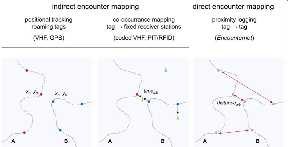
Two types of encounter mapping technology can be distinguished (see schematic in Fig. 1; [8]). With ‘indirect encounter mapping’, the spatiotemporal movements of tagged animals are tracked individually, and co-occur-rence patterns are inferred post hoc at the data analysis stage. This includes, for example, the use of VHF (very high frequency) radio-telemetry [9] or GPS (global posi-tioning system) logging [10] to locate animals (yielding time-stamped X and Y coordinates), or more recently, of PIT/RFID (passive integrated transponder/radiof-requency identification) tags [11] that are detected by a grid of stationary reading stations (yielding time-stamped visitation data). In contrast, ‘direct encounter mapping’ involves the use of animal-mounted tags—so-called proximity loggers (or ‘business card’ tags; [12])—that communicate with each other, to produce reciprocated records of social contacts (in the form of time-stamped encounter logs; Fig. 2). Direct encounter mapping can thus occur when animals associate away from fixed read-ing stations and in habitats where movement trackread-ing would be challenging (e.g. because forest cover limits the use of GPS). Proximity loggers are ‘transceiver’ tags that both transmit and receive radio signals (acoustic versions for aquatic habitats are available; [12, 13]) and exploit the fact that radio signals attenuate predictably with

distance. The technology can therefore be used to make inferences about the ‘proximity’ of associating individuals (see below, and for a detailed discussion, [14]), but data on the physical locations of encounters are usually lack-ing (but see [15, 16]). Georeferencing the data collected by proximity loggers remains a major challenge [16], but promises unprecedented insights into the spatiotemporal dynamics of a wide range of biological processes.

We have recently conducted the first full-scale deploy-ment of a novel proximity-logging system, “Encounter-net” (Encounternet LLC, Washington, Seattle, USA), to investigate the social networks of tool-using New Cal-edonian crows Corvus moneduloides. As explained in detail below, Encounternet is a fully digital proximity-logging technology, which unlike other commercially available terrestrial systems [17–22] enables tag-to-tag communication over distances well in excess of 10  m (other systems usually transmit over a few metres) and records raw signal-strength data for encounters [other systems record detections as binary (yes/no) data]. In earlier papers, we have described how we calibrated our system for field deployment [14] and reported the anal-ysis of both time-aggregated [23] and dynamic network data [15]. Here, we explain the basic procedures for pro-cessing and visualising proximity-logger data, focussing

indirect encounter mapping

direct encounter mapping

positional tracking roaming tags

(VHF, GPS)

co-occurrance mapping tag fixed receiver stations

(coded VHF, PIT/RFID)

proximity logging tag tag (Encounternet)

xb, yb

xa, ya timea/b

distancea/b

A B A B A B

specifically on Encounternet-unique features (for an ear-lier study on tags developed by Sirtrack Ltd., see [24]) and on some subtleties that may be easily overlooked by first-time users. Taken together, our four papers [14, 15, 23,

this study] provide a comprehensive description of how to use Encounternet and similar wireless sensor network (WSN) technology [25, 26], to study the social dynamics of free-ranging animals.

Transmitter

ID ReceiverID Start End Duration

A B

B A

83

68

143

168

60

100

a

c

b

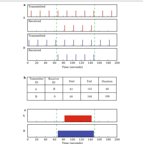
Fig. 2 Schematic illustrating the recording and basic interpretation of proximity-logging data. a Proximity loggers are transceiver tags that both transmit and receive radio signals (see main text). In this hypothetical example, tags A and B transmit radio pulses every 20 s and are within reception range of each other between t₁= 65 s and t₂= 150 s, indicated by green dashed lines. b Simplified log file showing how the encounter is recorded in the tags’ memories (for a sample of a genuine log file, see Table 1). c At the analysis stage, the encounter between A and B can be reconstructed from their respective log files. The upper plot shows the encounter according to what tag A received, and the lower plot according to what tag B received. The disparity in start and end times for the encounter, as recorded by A and B, arises from the difference in times at which tags

Methods

Proximity‑logging technology

The Encounternet system consists of animal-mounted loggers (henceforth ‘tags’ for simplicity) and a grid of fixed receiver stations (‘basestations’), which are used for downloading data remotely from tags (for photos of hard-ware, see [14]). Each tag emits uniquely ID-coded radio pulses at regular, user-defined time intervals (here 20 s; see below) and continually ‘listens’ for the signals of other tags. When two tags come within reception range of each other, each tag opens a log file which records data about the encounter—the received ID code, the start and end times of the encounter and a measure of signal strength (for sample data, see Table 1). These data comprise a ‘reciprocated encounter’. An example of the timings of pulses transmitted and received by two tags during an encounter is shown schematically in Fig. 2a, b illustrates how data would be logged by each tag. Without inde-pendent knowledge of the timings of pulses, the encoun-ter would be reconstructed from the log files as shown in Fig. 2c. Figure 2 demonstrates that a phase offset between the transmission times of the two tags can cause a dispar-ity in the start and end times of the encounter recorded by each tag (but this should be less than the programmed pulse interval).

During an encounter, signal strength is recorded as a ‘received signal-strength indicator’ (RSSI) value, which is a measure of the power ratio (in dB) of the received signal and an arbitrary reference (for details, see [14]); the RSSI value is converted to an integer for recording and will henceforth be unitless. For each encounter log, which consists of (up to) a pre-programmed number of consec-utively received radio pulses, the minimum, maximum and mean RSSI (RSSImin, RSSImax and RSSImean) values of

the pulse sequence are recorded (Table 1). The proximity of the tags can later be estimated from RSSI values using an appropriate calibration curve [14, 27].

In the present study, we programmed tags to emit pulses every 20  s, which is significantly less than the

timescales over which crows’ fission–fusion dynamics are expected to occur (minutes to tens of minutes; see [23]). Tags are unable to receive signals during the brief peri-ods (several milliseconds) when they are transmitting, so although slight differences in on-board clock times (gen-erated by tag-specific drift rates) ensured that phase syn-chrony was unlikely, the exact transmission times were jittered by multiples of 1/3 s up to ± 4/3 s to minimise this possibility.

Field deployment

In October 2011, we deployed Encounternet tags on 41 wild New Caledonian crows in one of our long-term study populations (for biological rationale of the study, see [23], and for background on the study species, see [28]); four tags failed after 4–11  days of transmission and a further four yielded no data, leaving 33 birds for analysis. Tags were attached to crows using weak-link harnesses which were designed to degrade over time, to release devices after the study. The data were collected via 45 basestations deployed in the study area. We have provided a full description of our field procedures else-where [15, 23].

Results

Preliminary data processing and analysis

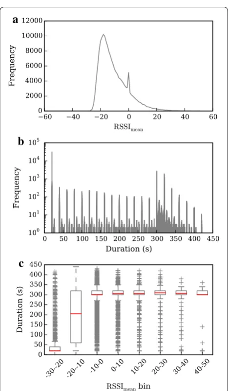
Data were recorded for 19  days, amassing ca. 240,000 encounter logs, with all 33 crows participating in at least one association. The encounters analysed (both here and in [15]) were restricted to those recorded between sunrise and sunset only, which constituted a sample of ca. 177,000 logs. Recorded RSSI values ranged from −61 to +60, corresponding to distances of over 50  m to within 1  m (for calibration results, see [14]). The distribution of RSSImean values for all encounter

logs is shown in Fig. 3a; the sharp peak at RSSImean = 0

was caused by a bug in the tags’ firmware [23] and is not due to the behaviour of the tagged animals, as suggested by another study [29].

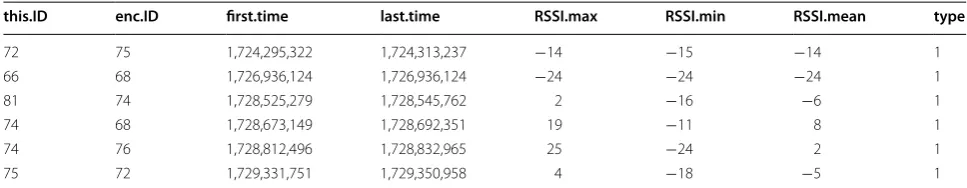
Table 1 Sample encounter logs recorded by crow-mounted “Encounternet” proximity loggers

‘this.ID’ and ‘enc.ID’ are the identities of the receiving and transmitting tags, respectively; ‘first.time’ and ‘last.time’ are the start and end time of an encounter (recorded in tag-clock units of 1/64 s); the following three ‘RSSI’ columns give signal-strength statistics for the pulse sequence making up the encounter; and ‘type’ codes distinguish, among other things, tag-to-tag logs (type = 1) from error messages and master node commands (not applicable in this example)

this.ID enc.ID first.time last.time RSSI.max RSSI.min RSSI.mean type

72 75 1,724,295,322 1,724,313,237 −14 −15 −14 1

66 68 1,726,936,124 1,726,936,124 −24 −24 −24 1

81 74 1,728,525,279 1,728,545,762 2 −16 −6 1

74 68 1,728,673,149 1,728,692,351 19 −11 8 1

74 76 1,728,812,496 1,728,832,965 25 −24 2 1

The distribution of encounter log durations is shown in Fig. 3b. The peaks at multiples of 20 s are a result of the tags’ programmed pulse rate (see above and Fig. 2). Tags created a single log for each encounter up to a maxi-mum of 15 received pulses, giving a peak in recorded log durations at 300 s. Because pulses could occasionally be missed (for example, because of a temporary obstruction between the birds), tags did not ‘close’ encounter logs until no pulse had been received from the other tag for

six consecutive pulse intervals (6 × 20 s = 120 s); when this occurred, the end time was recorded as the time of the last received pulse. There is thus a second peak at 320 s (one missed pulse during the encounter), a smaller one at 340 s (two missed pulses) and so on. If more than 15 pulses were received during an encounter, successive log files were created. Grouping encounter log dura-tions by 10-point RSSImean bins reveals that long-distance

encounters are much shorter than close-range ones (Fig. 3c).

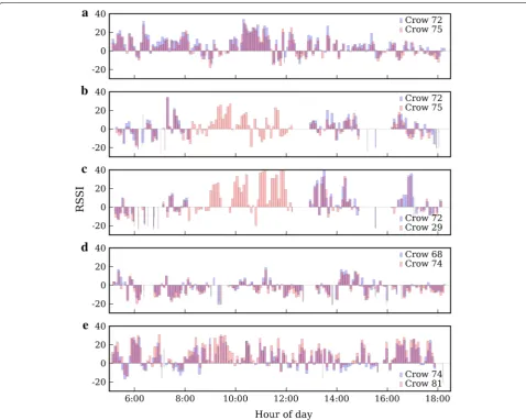
Figure 4 contains a simple visualisation of a day’s worth of encounter logs for two different pairs of crows. It can be seen that there is considerable variation in signal strength from one encounter log to the next, and that reciprocated encounter logs do not match exactly either in timing or in signal strength. The majority of encoun-ter logs appear to have roughly the same duration (ca. 300  s, as per our pre-programmed 15-pulse limit), and successive encounter logs are separated by a small gap of around 20  s (more easily visible in Fig. 5), which is another consequence of tags emitting a pulse every 20 s.

Filtering and amalgamation of reciprocated encounter logs Spatial proximity is a symmetric proxy for association; if crow A is 10 m from crow B, then crow B is also 10 m from crow A. The logs recorded by the tags, however, are not perfectly symmetrical; for example, there will be vari-ation in the transmitting and receiving strength of tags. Details of the factors influencing signal strength can be found in [14]. Here, we concentrate on the steps taken to clean the data, whatever the cause of the discrepancies.

In Fig. 6, we illustrate the recorded RSSImean values of

reciprocated encounter logs between five different pairs of crows on chosen days. Each plot shows the signals received by each tag of a pair plotted in red or blue. The five examples illustrate a range of ways in which recip-rocated signals can differ. The first type of discrepancy is that one tag in a pair can consistently record a higher signal strength than the other (Fig. 6a, e). All five exam-ples show that the start and end times of encounter logs can differ. In some instances, it was actually impossible to match up pairs of encounter logs between the tags. Dif-ferences in encounter log duration can be seen most eas-ily in Fig. 6e, between 9:00 and 10:00 hours where tag #74 (blue) records encounter logs with much shorter dura-tion than tag#81 (red). Lastly, Fig. 6b, c shows encounter logs for two crow dyads, both involving crow #72 (blue in both plots), which did not contribute any data during the latter half of the morning.

To construct a symmetric set of encounters from the data, reciprocated signals must be amalgamated to pro-duce a single timeline of encounters between each pair of crows. Since there were no calibration experiments

a

b

c

performed to assess variation in tag performance (includ-ing output power and reception sensitivity; see [30, 31]), there is no way of reliably determining the ‘correct’ sig-nal strength for encounters. The lack of tag-specific cali-bration also makes it impossible to know which tags are more accurately recording start and end times of encoun-ters. In addition to these issues, nothing is known about the height of tags above the ground, the relative orienta-tion of the two tags (and their antennae), or the habitat where the encounter took place, all of which affect RSSI

(for details, see [14, 23]). We have therefore used a sim-ple method of reconciling reciprocated encounter logs, which does not require any independent information on these factors.

The first step in amalgamating reciprocated encounter logs is to apply a filter criterion (FC), so that only logs that are likely to result from encounters of biological interest are retained for further analyses. In our study of social dynamics in New Caledonian crows, we were pri-marily interested in close-range encounters of birds [23],

Fig. 4 Examples of encounter logs for two crow dyads during daylight hours. The two examples illustrate patterns for pairs of crows that associated (a) frequently [encounter data on day 15, between crows #74 and #81, as recorded by tag 74# (blue) and tag #81 (red)]; and (b) only sporadically [encounter data on day 2, between crows #84 and #85, as recorded by tag #84 (blue) and tag #85 (red)]. Each encounter log is shown as a shaded bar, extending horizontally from the start to end time of the log, and vertically from the minimum to the maximum RSSI values recorded during the encounter; between RSSImin and RSSImean, the bars are shaded in light blue or red, and from RSSImean to the RSSImax the bars are shaded in a darker

and after system calibration, settled on an FC of RSSImean

≥15; for single radio pulses, we estimated through simu-lation that 50 % of pulses of an RSSI ≥15 will result from an inter-tag distance of 4.74 m or less, while 95  % of pulses will originate from within 11.29 m (for details, see [14]). Over distances of a few metres, we would expect crows to be able to observe, and socially learn from, each other, which is key for the biological process we hoped to elucidate—the possible diffusion of foraging inventions across crow networks.

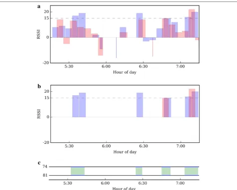
The steps taken to amalgamate reciprocated encounter logs are shown in Fig. 5 for real Encounternet data from tags #74 and #81, collected between 5:15 and 7:15 hours

on day 14. In this example, we have amalgamated the RSSImean values of signals transmitted by tag #74 and

received by tag #81 (shown in blue) with signals trans-mitted by tag #81 and received by tag #74 (shown in red) (Fig. 5a). After discarding all encounter logs which do not meet the chosen FC, this leaves eight periods of associa-tion, six received by tag #81 and two by tag #74 (Fig. 5b). The first two shortly after 5:30 hours are an example of two bouts separated by a brief gap (Fig. 5b). As men-tioned in the previous section, this is a result of the pro-grammed limit of log files, to close after a maximum of 15 consecutively received 20-s pulses (=300 s). To be able to analyse the total length of time in which crows remain

within range, we have concatenated consecutive encoun-ter logs which are separated by a gap of less than 23 s (to account for the 20-s gap between pulses and give an extra 3-s ‘leeway’ to ensure that consecutive logs will be con-catenated). Data processing resulted in four encounters (meeting the FC) between crows #74 and #81, as illus-trated in the ‘timeline’ plot in Fig. 5c. In such plots, the timeline of a crow is represented by a black horizontal line, and green shading between two timelines indicates a period in which the two crows are engaged in an encoun-ter (cf. Fig. 7). We note that, by defining an ‘encounter’ as a period when at least one tag in a dyad logs a signal

strength above our FC, we retain some encounters in which one of the tags logs below the FC. This is justified, since there are many ways that environmental conditions can cause a radio signal to weaken [14, 26], but few ways a signal can be boosted; false positives are therefore highly unlikely, while false negatives will occur frequently.

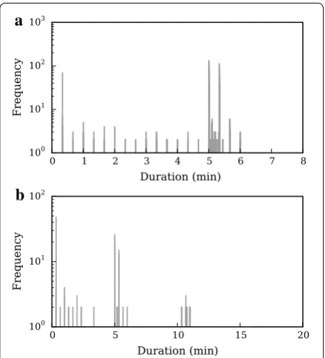
Figure 8 shows the effect of amalgamating encounter logs on the distribution of durations for our Encounternet deploy-ment. Whilst the majority of encounters are between 5 and 6 min long, amalgamation at an FC of RSSImean≥15 revealed

that crows spent up to ca. 11 min in close proximity of each other. The median 5-min encounter duration corresponds to

the programmed 15-received pulse limit of log files. In many of these encounters, crows will have been close to each other for more than 5 min, but the logs recorded before and after this log will have failed to meet the FC, because the mean RSSI was ‘dragged down’ by pulses received when the birds were first approaching each other, and then, having closely associated, separating from each other.

Temporal network visualisation

The complete temporal dataset of amalgamated encoun-ters can be displayed on timeline plots for all crows (cf.

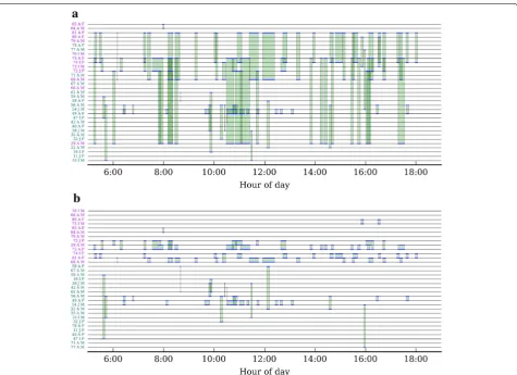
[32]). Figure 7 shows such a plot for 1  day’s worth of encounters. Ordering crows according to ascending tag ID is not visually appealing, as many encounters (green shading) overlap with each other (Fig. 7a). One way to improve data visualisation is to place the timelines of

frequently associating crows close together. An optimal ordering of the crows can be found by minimising the total area of green shading on each plot, as we have illus-trated here for the first 7 days of our deployment (Fig. 7b; during which the population was not subjected to experi-mental manipulations; see [15]). It is easy to see that this layout makes the structure of the data much more apparent; for example, there are several pairs or triplets of crows (e.g. adults #81 and #68, and immature #74) which engage in close-range encounters with each other throughout the course of the day, suggesting that these crows have strong social bonds.

Discussion

Research projects using proximity-logging systems pro-ceed through three major stages: system preparation

Fig. 7 Dynamic encounter data for a population of wild New Caledonian crows. Timeline plots showing all encounters with RSSImean≥15 on day 7. The timeline of each crow is represented by a horizontal line, with green shading between two timelines indicating the period during which the two individuals were engaged in an encounter (cf. Fig. 5c). Each timeline is labelled with tag ID, age (J juvenile; I immature; A adult) and sex (F female;

and calibration; field deployment and data collection; and data processing and analysis. Prospective users of this technology need to be aware that each of these steps will remain a major undertaking, until hardware, field procedures and analysis techniques have become more established. In this paper, we have offered some guidance on aspects of data processing and visualisation. Once deployed, proximity-logging systems can quickly gener-ate vast amounts of data, which may take some users by surprise (especially, those that have no prior experience with biologging technologies). It is essential that research teams possess sufficient bioinformatics expertise as well as adequate infrastructure for data storage and handling.

While aspects of data cleaning and processing have been described previously (e.g. [18, 24, 30, 31]), these studies were concerned with proximity-logging systems that record encounters as binary detection data (such as the proximity tags by Sirtrack Ltd., New Zealand). In con-trast, we provide the first description of techniques for a system that records raw signal-strength (i.e. RSSI) values and, therefore, enables post hoc data filtering by signal strength—and hence animal-to-animal distance—at the analysis stage. To allow further refinements of filtering procedures, we recommend that future studies quantify each tag’s transmission power before deployment [30],

as such variation could cause animals to appear more or less sociable than they really are [31]. Alternatively, field-recorded data could be used to assess the differ-ence in RSSI values recorded by pairs of tags; comparison of RSSI frequency distributions may reveal differences in tag performance that could be taken into account in subsequent analyses. Our study also illustrated how cer-tain data properties, such as encounter durations, are influenced by tag settings (such as pulse intervals; Fig. 3) and processing procedures (such as amalgamation and concatenation criteria; Fig. 8). When embarking on a proximity-logging project, it is important to recognise how this can potentially affect the biological conclusions that are being drawn from the data. Where possible, we encourage: pilot testing of parameter settings before field deployment, to ensure that they are suitable for map-ping the biological processes of interest (e.g. [23]), and detailed sensitivity analyses at the data-mining stage, to confirm that key results are robust (e.g. [15]).

In many study contexts, well-established, indirect encounter mapping technologies (see “Background”; Fig. 1) will remain the method of choice; for example, for species living in open habitats, conventional GPS track-ing systems can provide high-resolution datasets that are straightforward to analyse. Where proximity logging is the best option, however, its strengths should be rec-ognised and fully exploited. First, being WSNs, data can be harvested remotely from roaming ‘nodes’ (animal-mounted tags) using fixed nodes (basestations) [25, 26], which create opportunities for near real-time analyses. In our study on New Caledonian crows, we used this feature to assess network parameters on a daily basis, to ascer-tain that a stable equilibrium state had been reached [23], before conducting experimental manipulations that were designed to disturb the network topology [15]. Achiev-ing this level of experimental control would be impos-sible with most other data collection techniques, but requires careful preparation of data-handling protocols and computer hard- and software resources, to enable ad hoc analyses under field conditions. Another strength of proximity-logging systems is the high temporal data res-olution they can achieve. With encounter ‘checks’ several times per minute for all tagged subjects, sampling rates exceed those possible with unaided field observation by several orders of magnitude. This increase in data qual-ity creates exciting opportunities for investigating social-network dynamics [4, 6–8, 15], but brings with it new challenges in terms of data visualisation. We have pro-vided examples of a timeline procedure (cf. [4, 32]), which we have found useful in our own work, as it enabled us to examine our full dataset in an intuitive way and plan more elaborate diffusion simulations ([15]; James et  al. unpubl. manuscript).

a

b

Conclusions

Proximity logging promises unprecedented insights into the social organisation of wild animals. We hope that the present paper will help prospective users recognise some of the pitfalls inherent in basic data analyses, which must be avoided to reach valid biological conclusions.

Abbreviations

ASN: animal social network; FC: filter criterion; GPS: global positioning system; PIT: passive integrated transponder; RFID: radiofrequency identification; RSSI: received signal-strength indicator; VHF: very high frequency; WSN: wireless sensor network.

Authors’ contributions

All authors contributed to the development of ideas. CR and JSC conducted fieldwork, and RJ and EB conducted data analyses. EB and CR drafted the manuscript, and all authors contributed to the final version. All authors read and approved the final manuscript.

Author details

1 _{Department of Physics and Centre for Networks and Collective Behaviour,}

University of Bath, Bath BA2 7AY, UK. 2 _{Department of Zoology, University}

of Oxford, Oxford OX1 3PS, UK. 3 _{Present Address: Centre for Biological}

Diver-sity, School of Biology, University of St Andrews, St Andrews KY16 9TH, UK.

Acknowledgements

We thank: T. Mennesson and the late C. Lambert for logistical support in New Caledonia; the Province Sud, SEM Mwe Ara and the DENV for research permits, access to land and facilities, and other help; the field team for assistance; and the BBSRC (Grants BB/G023913/1 and/2 to CR) and the University of Bath (studentship to EMB) for funding.

Compliance with ethical guidelines

Competing interests

The authors declare that they have no competing interests.

Received: 25 March 2015 Accepted: 11 August 2015

References

1. Croft DP, James R, Krause J (2008) Exploring animal social networks. Princeton University Press, Princeton

2. Whitehead H (2008) Analyzing animal societies. Chicago University Press, Chicago

3. Krause J, James R, Franks DW, Croft DP (eds) (2014) Animal social net-works. Oxford University Press, Oxford

4. Blonder B, Wey TW, Dornhaus A, James R, Sih A (2012) Temporal dynamics and network analysis. Methods Ecol Evol 3:958–972

5. Kurvers RHJM, Krause J, Croft DP, Wilson ADM, Wolf M (2014) The evolu-tionary and ecological consequences of animal social networks: emerg-ing issues. Trends Ecol Evol 29:326–335

6. Pinter-Wollman N, Hobson EA, Smith JE, Edelman AJ, Shizuka D, de Silva S, Waters JS, Prager SD, Sasaki T, Wittemyer G, Fewell J, McDonald DB (2014) The dynamics of animal social networks: analytical, conceptual, and theoretical advances. Behav Ecol 25:242–255

7. Sih A, Wey TW et al (2014) Dynamic feedbacks on dynamic networks: on the importance of considering real-time rewiring—comment on Pinter-Wollman et al. Behav Ecol 25:258–259

8. Krause J, Krause S, Arlinghaus R, Psorakis I, Roberts S, Rutz C (2013) Reality mining of animal social systems. Trends Ecol Evol 28:541–551

9. Kenward RE (2001) A manual for wildlife radio tagging. Academic Press, London

10. Cagnacci F, Boitani L, Powell RA, Boyce MS (2010) Animal ecology meets GPS-based radiotelemetry: a perfect storm of opportunities and chal-lenges. Phil Trans R Soc B 365:2157–2162

11. Bonter DN, Bridge ES (2011) Applications of radio frequency identification (RFID) in ornithological research: a review. J Field Ornithol 82:1–10 12. Holland KN, Meyer CG, Dagorn LC (2009) Inter-animal telemetry: results

from first deployment of acoustic ‘business card’ tags. Endang Species Res 10:287–293

13. Guttridge TL, Gruber SH, Krause J, Sims DW (2010) Novel acoustic technology for studying free-ranging shark social behaviour by recording individuals’ interactions. PLoS One 5:e9324

14. Rutz C, Morrissey MB, Burns ZT, Burt J, Otis B, St Clair JJH, James R (2015) Calibrating animal-borne proximity loggers. Methods Ecol Evol 6:656–667 15. St Clair JJH, Burns ZT, Bettaney EM, Morrissey MB, Burt J, Otis B, Ryder TB,

Fleischer RC, James R, Rutz C (2015) Experimental resource pulses influ-ence social-network dynamics and the potential for information flow in tool-using crows. Nat Commun (in press)

16. Picco GP, Molteni D, Murphy AL, Ossi F, Cagnacci F, Corrà M, Nicoloso S (2015) Geo-referenced proximity detection of wildlife with WildScope: design and characterization. In: Proceedings of the 14th ACM/IEEE inter-national conference on information processing in sensor networks (IPSN 2015)

17. Ji W, White PCL, Clout MN (2005) Contact rates between possums revealed by proximity data loggers. J Appl Ecol 42:595–604 18. Prange S, Jordan T, Hunter C, Gehrt SD (2006) New radiocollars for the

detection of proximity among individuals. Wildl Soc Bull 34:1333–1344 19. Böhm M, Palphramand KL, Newton-Cross G, Hutchings MR, White PCL (2008) Dynamic interactions among badgers: implications for sociality and disease transmission. J Anim Ecol 77:735–745

20. Böhm M, Hutchings MR, White PCL (2009) Contact networks in a wildlife-livestock host community: identifying high-risk individuals in the transmission of bovine TB among badgers and cattle. PLoS One 4:e5016 21. Hamede RK, Bashford J, McCallum H, Jones M (2009) Contact networks

in a wild Tasmanian devil (Sarcophilus harrisii) population: using social network analysis to reveal seasonal variability in social behaviour and its implications for transmission of devil facial tumour disease. Ecol Lett 12:1147–1157

22. Weber N, Carter SP, Dall SRX, Delahay RJ, McDonald JL, Bearhop S, McDonald RA (2013) Badger social networks correlate with tuberculosis infection. Curr Biol 23:R915–R916

23. Rutz C, Burns ZT, James R, Ismar SMH, Burt J, Otis B, Bowen J, St Clair JJH (2012) Automated mapping of social networks in wild birds. Curr Biol 22:R669–R671

24. Watson-Haigh NS, O’Neill CJ, Kadarmideen HN (2012) Proximity log-gers: data handling and classification for quality control. Sens J IEEE 12:1611–1617

25. Ceriotti M, Chini M, Murphy AL, Picco GP, Cagnacci F, Tolhurst B (2010) Motes in the jungle: lessons learned from a short-term WSN deployment in the Ecuador cloud forest. In: Proceedings of the 4th international work-shop on real-world wireless sensor networks applications (REALWSN), pp 25–36

26. Marfievici R, Murphy AL, Picco GP, Ossi F, Cagnacci F (2013) How environ-mental factors impact outdoor wireless sensor networks: a case study. In: Proceedings of the 10th international conference on mobile ad-hoc and sensor systems (MASS), pp 565–573

27. Meise K, Krüger O, Piedrahita P, Mueller A, Trillmich F (2013) Proximity log-gers on amphibious mammals: a new method to study social relations in their terrestrial habitat. Aquat Biol 18:81–89

28. Rutz C, St Clair JJH (2012) The evolutionary origins and ecological context of tool use in New Caledonian crows. Behav Process 89:153–165 29. Mennill DJ, Doucet SM, Ward K-AA, Maynard DF, Otis B, Burt JM (2012)

A novel digital telemetry system for tracking wild animals: a field test for studying mate choice in a lekking tropical bird. Methods Ecol Evol 3:663–672

30. Boyland NK, James R, Mlynski DT, Madden JR, Croft DP (2013) Spatial proximity loggers for recording animal social networks: consequences of inter-logger variation in performance. Behav Ecol Sociobiol 67:1877–1890

31. Drewe JA, Weber N, Carter SP, Bearhop S, Harrison XA, Dall SRX, McDonald RA, Delahay RJ (2012) Performance of proximity loggers in recording intra-and inter-species interactions: a laboratory and field-based valida-tion study. PLoS One 7:e39068