Economics Working Paper Series
2016/015
Push or Pull? Performance Pay, Incentives, and
Information
David Rietzke and Yu Chen
The Department of Economics Lancaster University Management School
Lancaster LA1 4YX UK
© Authors
All rights reserved. Short sections of text, not to exceed two paragraphs, may be quoted without explicit permission,
provided that full acknowledgement is given.
Push or Pull? Performance Pay, Incentives, and
Information
∗
David Rietzke
†and Yu Chen
‡September 7, 2016
Abstract
We study a principal-agent model wherein the agent is better
in-formed of the prospects of the project, and the project requires both
an observable and unobservable input. We show (1) Performance pay
may not be optimal, even if output is the only informative signal of
an essential input; (2) Total surplus tends to be higher if one input is
unobservable than if both inputs are observable; and (3) Bunching may
arise amongst low and intermediate types. We explore the implications
for push and pull programs used to encourage R&D activity, but our
results have applications beyond this context.
KEYWORDS: Pay for Performance, Moral Hazard, Adverse Selection, Observable Action, Principal-Agent Problem, Grants, Prizes
JEL Classifications: D82, D86, O31
∗A previous working paper was issued under the title, “Push or pull? Grants, prizes, and
information”. We thank Stan Reynolds, Andreas Blume, Asaf Plan, John Wooders, Mar-tin Dufwenberg, Rabah Amir, Derek Lemoine, Brian Roberson, Junichiro Ishida, Matthew Mitchell, Tim Flannery, and Dominik Grafenhofer for helpful comments and suggestions. We also thank participants at the Lancaster University Conference on Auctions, Competi-tion, RegulaCompeti-tion, and Public Policy, The EARIE Annual Conference, The Royal Economics Society Annual Conference, and the TILEC Conference on Competition, Standardization, and Innovation.
1
Introduction
To what extent should incentives be tied to performance? This question is relevant in a number of areas, including worker compensation – where it relates to the debate on salaries vs. piece rates (see, e.g. Lazear, 1986, 2000) – and innovation incentives, where it pertains to the efficacy of “push” and “pull” programs (see, e.g., Kremer, 2002). Push programs, such as research grants, or R&D tax credits, subsidize research input; payments are not contingent on results. Pull programs, such as innovation prizes, or patent buyouts, directly tie rewards to research output.
Adverse selection (AS) and moral hazard (MH) are inherent challenges in the provision of incentives. Given these problems, Kremer raises the concerns that push programs may reward researcher’s unlikely to succeed, and provide weak incentives for unobservable inputs. Indeed, the literature on MH stresses the importance of performance pay. In the canonical MH model,1 the agent’s
effort is unobservable by the principal, but output, a noisy signal of effort, is observable. In that model, compensation must be at least partially tied to output to provide an incentive for greater effort. More generally, H¨olmstrom’s (1979) “informativeness principle” implies that it is valuable for the principal to condition rewards on any signal – including output – that provides addi-tional information about the agent’s effort.
Despite these concerns, “low-powered” incentive schemes, in which com-pensation is weakly, or not at all tied to performance, are commonly used in practice. In this paper, we offer a new justification for the use of such schemes. We show that when AS and MH interact, and at leastsome of the agent’s ac-tions are observable, performance pay may not be optimal, even if output is the only informative signal of an essential input.
For concreteness, we present our model in the context of R&D funding, but our results are relevant in other contexts. We study a principal-agent model wherein a risk-neutral funder (he; the principal) incentivizes a risk-neutral researcher (she; the agent) to undertake an R&D project, which may yield a
new technology. The likelihood of success depends on the researcher’s privately known type, and two essential and complementary inputs – “investment” and “effort”. Investment is observable by the funder; effort is not.2 If she succeeds,
the researcher earns a profit by marketing the technology, but this incentive, alone, may be insufficient to elicit R&D activity.3 To ensure the researcher has
an incentive to truthfully reveal the project’s outcome, the funder is subject to a “free-disposal” constraint, stipulating that the reward for success is no less than the reward for failure.
The contracts offered by the funder consist of a transfer independent of performance – a “grant” – and a payment for success – a “prize”. The prize and grant may depend on investment, but neither can depend on effort. We show (i) Performance pay may not be optimal; (ii) Total surplus tends to be higher when effort is unobservable, than when it is observable; and (iii) Bunching may arise amongst low and intermediate types.4
We briefly describe the intuition for our results. (i) The prize creates a strong incentive for effort, but generates costly information rent for the researcher due to AS. As a result of this tradeoff, the prize may be zero for all, or a subset of types. In these cases, the researcher’s compensation is completely independent of her performance. Effort is induced indirectly, through the grant. The grant is used to encourage greater investment, which increases the productivity of effort. The researcher’s product-market profit may then provide a sufficient incentive for effort.
(ii) If both inputs are observable, then investment is distorted below the first-best to limit the researcher’s information rent. When effort is unobserv-able, a larger investment and/or a prize may be necessary to induce effort. But it is advantageous for the funder to raise investment closer to the first-best. Doing so increases the researcher’s rent, but increases total surplus, which
2Throughout this analysis, we use the terms “observable”, “contractible”, and
“verifi-able” interchangeably.
3In a more general setting, this incentive might reflect the prospect of a future outside
job opportunity, or some intrinsic motivation.
4Bunching refers to a situation where the principal offers the same contract to multiple
partially offsets the additional cost to the funder. A prize, in contrast, simply transfers surplus from the funder to the researcher. For this reason, investment and total surplus are (weakly) greater when effort is unobservable than when it is observable.
(iii) Bunching may arise amongst low and intermediate types due to a tension between rent extraction, effort inducement, and the second-order in-centive compatibility constraint. As this is a more technical point, we defer a discussion of this finding to Section 4.4.
The main contributions of our analysis are twofold. First, we add to the literature on contracting. Following the tradition of the canonical MH model, most mixed models assume a production process that depends only on unob-servable actions.5 But this premise is rather extreme. The mental or physical
effort of an agent may be prohibitively costly to monitor, or even quantify. But investments by a firm in large-scale capital, or the time a worker spends at work, are quantifiable, and likely easier to verify. We add to this literature by providing a full characterization of the optimal incentive scheme in a setting with AS, and inputs that consist of both an observable and unobservable com-ponent. We show that the partial observability of these inputs has dramatic consequences for the structure of optimal incentives, and interesting welfare implications.
If only output is observable then rewards cannot depend on actions(s), and performance pay is essential. A payment received independent of performance affects the agent’s overall utility, but will not generate greater marginal incen-tives. This need not be the case when actions are partially observable. If, for instance, a researcher’s investment in capital is observable, then rewards can be directly tied to this input, and greater investment can be encouraged. But it may be that the researcher’s effort is more productive when she has better equipment with which to work. If so, then as long as there is some benefit to success, greater investment increases the marginal returns to effort, and thus,
5Early examples in the literature include Sappington (1982) and Picard (1987). Studies
effort is encouraged without tying rewards to performance.6 This observation
relates closely to findings by H¨olmstrom and Milgrom (1991). When the agent undertakes multiple tasks and efforts are complements, the authors show that a stronger incentive for effort on one task, simultaneously induces a higher effort on some other task.
H¨olmstrom and Milgrom provide an alternative explanation for rewards independent of performance. Their finding relies on actions being substitutes,7
and the lack of an informative signal associated with some action. Our result relies on a complementarity between actions, the presence of an observable action, and the interaction between AS and MH. Additionally, the “fixed wage” in H¨olmstrom and Milgrom’s model is a transfer independent of any signal received by the principal, while the grant depends on the observable action, but is independent of output. This grant structure better captures the design of many incentive schemes used in practice. The U.S. R&D tax credit system, for example, rewards firms independently of performance, but the value of the credit is directly tied to R&D investment. Similarly, an hourly worker’s wage may not be contemporaneously tied to performance, but she is only paid for the time she spends at work.
Meng and Tian (2012) study a multitasking model with AS and MH, and provide conditions under which lower-powered incentives arise, as compared to pure MH. We provide conditions under which optimal incentives are completely independent of performance. When the principal faces a multidimensional AS problem, Meng and Tian also show that optimal compensation may be inde-pendent of some performance measures. But their result differs fundamentally from our’s. In their model the agent undertakes multiple tasks, each of which contribute to the principal’s payoff. For those tasks where the performance measures are ignored, the agent exerts no effort. Thus, Meng and Tian’s result explains why an agent may be lead to specialize on certain tasks. In our model
6In the context of worker compensation, it might be that the (unobservable) mental effort
the worker devotes to her job is more productive when she spends more time at work.
7The so-called “effort substitution problem”. In this case, a stronger incentive for effort
there is a single task that requires multiple inputs. We show why incentives might be independent of the outcome of that task, even if this is the only verifiable signal associated with an essential input.
Our results also shed new light on the welfare implications of AS and MH. As this literature is quite extensive, we provide only a brief summary here; a more thorough overview may be found in Laffont and Martimort (2009, Ch. 7). In some models, adding MH creates no further welfare losses, as compared to pure AS.8 In many other settings, the AS and MH problems exacerbate one
another, leading to greater welfare losses than pure AS or pure MH. Laffont and Martimort emphasize that this is a quite common feature of models, such as our’s, where “MH follows AS”.9 Basov and Bardsley (2005) present an
example that follows a similar setup to our model, but without an observable action. They show that the first-best can be achieved under pure AS or pure MH, but distortions arise in the combined case.10 In contrast, we show that
there may be welfare gains to adding MH (relative to pure AS) in these models when actions are partially observable.
Laffont and Martimort discuss another class of models – those where AS follows MH11 – in which adding MH may improve welfare, relative to pure
AS. In these models, with pure AS distortions arise to limit the agent’s rent. But when MH is added, it is this rent at the AS stage that motivates greater effort at the MH stage. So, under AS and MH, the principal may reduce distortions in order to raise the agent’s rent, and encourage greater effort. In our model MH follows AS, so it is not the rent captured at the AS stage that motivates greater effort. Rather, the agent’s optimal effort depends directly on her investment; to elicit effort under AS and MH, investment is raised closer to the socially optimal level.
Our second contribution is to the literature on innovation incentives. Many
8See, e.g., Laffont and Tirole (1986); Picard (1987); Guesnerie et al. (1989); Caillaud
et al. (1992). Basov and Bardsley (2005) show that independence between the agent’s type, and the noise in the production function is the basic assumption that lead to these findings.
9That is, the agent learns her type prior to choosing her unobservable action. 10See, also, Lewis and Sappington (2000b) and Gottlieb and Moreira (2015).
11In these models, the agent chooses an unobservable effort that stochastically determines
studies have explored the optimal design of pull programs (e.g., optimal patent design),12or compared the performance of different pull programs (e.g., prizes
vs. intellectual property).13 Fewer studies have examined the optimal design
of push programs, or attempted to justify their use, taking MH into account. Our results are useful in both respects. Further, we connect our results to the U.S. R&D tax credit system, and comment on its design.
Maurer and Scotchmer (2003) argue that repeated interaction between grantees and grantors resolves the MH problem. Our explanation for how a push program might overcome MH complements their’s, as it is relevant in a static setting. This is important because some push programs, such as R&D tax credits, do not condition eligibility for rewards based on past perfor-mance. Fu et al. (2012) show that grants may be useful for facilitating greater competition in a research contest where researchers have asymmetric capital endowments. We abstract from the effects of competition, in order to focus on the role of information.
A number of other explanations for the emergence of low-powered incentive schemes have been posited in other contexts. Baker (1992) shows that perfor-mance pay may be muted if output is not contractible, and weakly correlated with the available performance measure. Baker’s result may be important in settings where “success” and “failure” are difficult to define. Risk-sharing is also an important consideration. Pay-for-performance schemes place consid-erable risk on the agent when outcomes are uncertain. Push programs may serve as a means of risk sharing.14 We abstract from such considerations, as
both the researcher and funder are risk neutral. Still, in the canonical MH model, risk aversion, alone, cannot explain the emergence of a push program, where rewards are independent of performance. Prendergast (2002) shows that output-based pay may be beneficial if the principal is uncertain of the “correct” action an agent should take, while input-based pay is more relevant in less uncertain environments. But Prendergast allows costly monitoring of
12See Hall (2007) for an overview.
13See Maurer and Scotchmer (2003) for an overview.
effort; we stick closer to the traditional MH paradigm, and assume effort is prohibitively costly to monitor.
2
Additional Related Literature
Others have examined the role of observable actions in MH models. Zhao (2008) studies a multitasking model where some actions are observable and shows, in stark contrast to our findings, that optimal compensation depends solely on output signals. But in Zhao’s model, efforts and outcomes are inde-pendent, and the observable actions are not verifiable, which places restrictions on feasible contracts. In a setup similar to Zhao, Chen (2010) shows that if the observable actions are verifiable, then optimal compensation depends on both the observable actions and output signals. Chen (2012) generalizes this find-ing, allowing multiple agents and complementarities between efforts; Chen’s results are consistent with our findings in a pure MH setting. Crucially, neither Zhao nor Chen incorporate AS.
Other models have allowed for AS and both observable and unobservable actions. For instance, in a large class of models following Laffont and Tirole (1986), the agent exerts unobservable effort to reduce marginal cost, and then chooses an observable level of production. But these models are quite distinct from our setup. First, many of these models involve “false moral hazard” (see Laffont and Martimort, 2009, ch. 7). Second, in these models, the technology through which the agent reduces cost depends only on an unobservable action. It is not until after the MH problem is resolved, that the observable action is chosen. In our model, the production process depends on both types of actions, and they are chosen simultaneously. In a quite general framework with AS and observable/unobservable actions, Caillaud et al. (1992) provide conditions under which a mechanism can be implemented via a menu of linear contracts. Meng and Tian’s framework can accommodate observable actions, but they focus on the case where actions are all unobservable; none of their results explicitly depend on the existence of an observable action.
AS, MH, and a direct contractible input from the principal. LS’s framework differs from ours in several important respects. First, in LS there are multiple agents (at least two).15 Second, each agent in LS’s model faces a wealth
con-straint, which translates to a capital constraint in our model. In particular, if the agent has zero “wealth”, the grant must reimburse the full cost of invest-ment. We don’t impose a capital constraint; this is important, as we show that the optimal grant typically does not fully reimburse investment. Third, our model explicitly takes into account an incentive outside the principal-agent relationship that can motivate effort.
3
The Model
3.1
The Primitives
We study a principal-agent model between a funder and a researcher. The researcher undertakes a single R&D project, which may or may not lead to the development of a new technology. The inputs are investment, x ∈ R+,
and effort,y ∈ {0,1}; where,y = 1 indicates working hard and y= 0 denotes shirking. Investment is observable by the funder; effort is not.
The researcher’s type, θ, is a random variable drawn from a continuous distribution according to CDF, F, corresponding (smooth) PDF,f, with sup-port, Θ = [θ, θ] ⊂ [0,1], where θ > θ > 0. The researcher knows the true θ
while the funder knows only its distribution. θ may capture some privately known characteristic of the project and/or the researcher’s innate ability. Let
h(θ) = 1−fF(θ()θ) denote the inverse hazard rate; assume, for all θ ∈Θ, h0(θ)<0 and f(θ)>0.
Given x, y, and θ, the probability of success is θp(x, y). The function,
p:R2+ →[0,1], is increasing in each argument, and twice continuously
differ-entiable, with p(0,·) = p(·,0) = 0, and for all x, y > 0, p12(x, y) > 0. That
is, investment and effort are both essential for success, and they are
comple-15This provides the principal with an additional instrument that we do not consider;
ments. We let ρ(x) denote p(x,1), and we may then write, θp(x, y) = θyρ(x). We assumeρis strictly increasing, but there are diminishing marginal returns to investment: ρ0 > 0 and ρ00 < 0. It is useful to point out that ρ0 contains some information about the complementarity between x and y. Specifically, the stronger is the complementarity betweenx and y, the larger will beρ0.
If the researcher invests x and chooses effort, y, she incurs a total cost of
x+cy. If the project succeeds she earns a profit in the product market ofπ >0, and the funder captures a benefit, W > 0. Otherwise both receive nothing.
W might represent, for example, the consumer surplus associated with the technology. Absent intervention, a type-θ researcher’s expected payoff is,
Π(x, y, θ) = θyρ(x)π−x−cy.
We let (x(θ), y(θ)) = arg maxx≥0,y∈{0,1}Π(x, y, θ) denote the researcher’s opti-mal no-intervention investment and effort; and we let Π(θ) = Π(x(θ), y(θ), θ) denote her maximized profit. We assume throughout that if the researcher is indifferent between working hard and shirking, she will choose to work; to-gether with the strict concavity ofρ, this meansx(θ) andy(θ) are unique. Note that π may or may not provide a sufficient incentive to elicit R&D activity (i.e., it may be that x(θ), y(θ),Π(θ)>0 or x(θ) =y(θ) = Π(θ) = 0).
3.2
Feasible Contracts and the Funder’s Problem
The funder designs contracts to motivate greater R&D activity from the re-searcher. A contract specifies a grant, g ∈ R, a prize, v ∈ R, and an invest-ment, x∈R+. The grant is received by the researcher independent of success
or failure, while the prize is a received only if the project succeeds.16
The outcome of the project is initially observed only by the researcher, who reports the result to the funder. If she reports success, the outcome is
16Note thatg <0 orv <0 represent transfers from the researcher to the funder.
Further-more, note that it is without loss of generality that we focus on grants and prizes. In general, an optimal mechanism will specify a transfer,ts, in the event of success, and a transfer,tf, in
verifiable at zero cost. But, we assume that the researcher may shroud her success from the funder, if it is in her interest to do so. To avoid creating this incentive, we follow Innes (1990), and more recently, Poblete and Spulber (2012), and impose a free-disposal constraint, which requires that the reward for success is no less than the reward for failure, i.e., v ≥0.17
We focus, without loss of generality, on “investment-forcing contracts”, where the researcher is only eligible for the grant/prize if she follows through on the agreed-upon investment. Note that if the researcher deviates from the agreed-upon investment,x0, and instead choosesx6=x0, and effort, y, then her payoff is Π(x, y, θ)≤Π(θ). So, as long as her payoff when she follows through onx0 exceeds Π(θ), it is never optimal to deviate from this investment.
By the Revelation Principle, it suffices to consider direct mechanisms. The funder commits to a menu of contracts, m = {v(θ), g(θ), x(θ)}θ∈Θ, where v :
Θ→R+denotes a prize schedule,g : Θ→Rdenotes a grant schedule, andx:
Θ→R+denotes an investment schedule. Throughout this analysis we restrict
attention to continuous, and piecewise differentiable prize/grant/investment schedules. The researcher observes the menu, and if she participates, reports her type, ˆθ, to the funder. The funder then specifies an investment level, x(ˆθ), a prize, v(ˆθ), and a grant, g(ˆθ), according to the menu. If the researcher does not participate, she earns Π(θ).
After the contract is formed, the researcher chooses investment and effort, the outcome of the project is realized, and transfers are made accordingly.
For a particular contract, {v, g, x},18 the researcher’s payoff is,
y[θρ(x)(v+π)−c]−x+g
Let y∗(v, x, θ) denote the researcher’s optimal effort choice: y∗(v, x, θ) = arg maxy∈{0,1}{y[θρ(x)(v +π)−c]−x+g}. It holds,
17 Note that when the free-disposal constraint is satisfied and the researcher behaves
optimally, the environment is equivalent to one in which the funder may observe the outcome of the project directly. We therefore do not explicitly model the outcome-report game.
18Where it does not cause confusion, we will liberally abuse notation, and sometimes
let v ∈ R+, g ∈ R, and x ∈ R+ denote particular prize, grant, and investment amounts,
y∗(v, x, θ) = 1 ⇐⇒ θρ(x)(v+π)−c≥0. (1)
When it is clear, we suppress the arguments of the researcher’s optimal choice of effort, and simply write y∗. For a given menu, m = {v(θ), g(θ), x(θ)}
θ∈Θ,
the payoff to a researcher of type θ who reports ˆθ is,
u(ˆθ|θ) = θy∗ρ(x(ˆθ))
v(ˆθ) +π
−x(ˆθ)−cy∗+g(ˆθ).
We letu(θ)≡u(θ|θ). If the researcher reports her type truthfully, the funder’s payoff is,
φ(m) =
Z θ
θ
θy∗ρ(x(θ)) [W −v(θ)]−g(θ)
f(θ)dθ
If one interpretsW as the consumer surplus associated with the innovation, then the funder’s payoff can be interpreted as expected consumer surplus, less the expected cost of funding.19
For a given θ, x, andy, let total (or social) surplus, S(x, y, θ), be defined as the sum of the researcher’s and funder’s payoffs:
S(x, y, θ) =θyρ(x)(W +π)−x−cy
Replacing g(θ) by u(θ) we can write the funder’s payoff as follows:
φ(m) =
Z θ
θ
S(x(θ), y∗, θ)−u(θ)
f(θ)dθ (2)
Equation (2) makes clear that the funder’s payoff is expected total surplus less the expected payoff of the researcher. The funder’s problem is then,20
19In this R&D context, the funder might also value the profit to the researcher. The
qualitative nature of our conclusions generalize to such an environment, provided there is some social cost to raising funds, as in Laffont and Tirole (1986, 1993), or the funder values firm profits less than consumer welfare. The important point is that transfers from the funder to the researcher are costly to the funder.
20Note thaty∗(·) is a single-valued function, and so we do not need to include an effort
max m φ(m)
s.t. for all θ,θˆ∈Θ :
u(θ)≥Π(θ) (IR)
u(θ)≥u(ˆθ|θ) (IC)
x(θ)≥0; v(θ)≥0
The first constraint is individual rationality (IR), the second is incentive compatibility (IC), the third gives the non-negativity constraint on investment, and the free-disposal constraint.
We will assume throughout thatW is sufficiently large such that the funder would like to induce effort from a researcher of any type. To ensure that this is optimal for the researcher, using (1), we impose the constraint,θρ(x(θ))(v(θ)+
π)−c ≥ 0, on the funder’s problem. Under this constraint, it holds that
y∗(v(θ), x(θ), θ) = 1 for all θ. Then, using standard techniques (see, e.g., Laffont and Tirole, 1993, pp. 64 and 121), it can be shown that IC is satisfied if and only if, for all θ ∈Θ:
u0(θ) = ρ(x(θ))(v(θ) +π) (IC-F)
d dθ
ρ(x(θ))(v(θ) +π)
=ρ0(x(θ))(v(θ) +π)x0(θ) +ρ(x(θ))v0(θ)≥0 (IC-S)
θρ(x(θ))(v(θ) +π)≥c (IC-E)
effort. Appendix A shows that the IC and IR constraints provided above are sufficient to rule out such a profitable deviation ifx(θ)≥x(θ) or Π(θ) = 0.
In many contexts, it seems reasonable to think that the principal would like to induce greater activity on the project than what the agent would otherwise choose. One might expect this to be the case in the context of R&D, since the social value of an innovation often far exceeds the private value to the innovator (see, e.g., Hall et al., 2009). In this regard, it is natural to assume that W is large, relative toπ. Specifically, we assume for allθ ∈Θ,
W > h(θ)
θ π (A1)
It will be seen that Assumption (A1) is sufficient to ensure that, in equi-librium, the funder’s desired level of investment exceeds x(·).
Assumption (A1) is also useful for dealing with the possibility of “counter-vailing incentives”,21 which may arise when the agent’s outside option is type
dependent (as it is in our model). These issues are explored by Lewis and Sappington (1989),22 but under (A1), the issue does not arise in our model.
The following lemma proves useful in establishing this fact.
Lemma 1. Let {v(θ), g(θ), x(θ)}θ∈Θ satisfy (IC-F), free disposal: v(·) ≥ 0,
and suppose x(θ)≥x(θ) for all θ. If u(θ)≥Π(θ), then u(θ)≥Π(θ) for all θ.
The significance of Lemma 1 is that IC and free-disposal are sufficient to ensure that IR is satisfied so long as (i) IR is satisfied for the lowest type, and (ii) the funder desires an investment level greater than what the researcher would otherwise choose. We will show that when W is sufficiently large, and (A1) holds, point (ii) is satisfied. So, IR is satisfied if u(θ) ≥ Π(θ) (and IC is satisfied). In this case, the IR constraint resembles the usual one that is independent of the agent’s type. Note that as the funder’s payoff is strictly decreasing inu(·), this IR constraint binds at the optimum: u(θ) = Π(θ).
21Many AS models are structured in such a way that the agent has a systematic incentive
to either under or over report her type. Countervailing incentives refers to a situation where some types have an incentive to under report, while others have an incentive to over report.
For convenience, we assume Π(θ) = 0; but it is straightforward to generalize our results to the case where Π(θ)>0, so long as (A1) is satisfied. Integrating both sides of (IC-F), and setting u(θ) = Π(θ) = 0, we obtain,
u(θ) =
Z θ
θ
ρ(x(t))(v(t) +π)dt (3)
Taking expectations (with respect toθ) over both sides of (3), and integrating the RHS by parts yields,
Z θ
θ
u(θ)f(θ)dθ=
Z θ
θ
ρ(x(θ))(v(θ) +π)h(θ)f(θ)dθ.
Substituting the expression above into (2), we obtain the following relaxed version of the funder’s problem,23
max x(·),v(·)
( Z θ
θ
θρ(x(θ))[W +π]−x(θ)−c−ρ(x(θ))(v(θ) +π)h(θ)
f(θ)dθ
)
[P]
Subject to (IC-S), (IC-E), x(θ)≥0, and free-disposal, v(θ)≥0.
4
Results
This section provides a full characterization of the optimal funding contracts. We first study three benchmark settings: complete information, pure MH, and pure AS. Throughout the analysis we use lower-case letters (x, v, g, etc.) to denote arbitrary investments, prizes, grants, etc. and upper-case letters (X, V, G, etc.) to denote optimal solutions. We will say that a funding contract is a pure grant if v = 0 and g > 0, and we analogously define a pure prize.
23This problem is a relaxation of the funder’s true problem, as it does not fully
We will say that a funding contract is a hybrid if v > 0 and g > 0. Finally, define a type-θ’s information rent as u(θ)−Π(θ). But note that as her rent is strictly increasing in u(·) (for a fixed Π(θ)), we will often just refer to u(·) when discussing the researcher’s rent.
4.1
Complete Information
With complete information, the funder observes the trueθ, and investment and effort are both observable. Given θ ∈ Θ, the funder offers a forcing contract,
m={v, g, x, y}, stipulating both investment and effort to solve,
max
m {θyρ(x)(W +π)−x−cy−u(θ)} s.t.
u(θ)≥Π(θ) and v ≥0
We let (XF B(θ), YF B(θ)) denote the first-best investment and effort level, which solve the problem above. Since the funder’s payoff is decreasing inu(θ), the IR constraint, u(θ)≥Π(θ), binds at the optimum. Then, straightforward maximization yields, for W sufficiently large, YF B(θ) = 1, and XF B(θ) > 0 given by the solution to the following first-order condition:
θρ0(XF B(θ))(W +π) = 1 (FB)
Note that (XF B(θ), YF B(θ)) maximize total surplus at θ: The LHS of (FB) is the marginal social gain from investment, while the RHS is the marginal social cost of investment. Applying the implicit function theorem to (FB), the concavity of ρ implies X0
F B(θ)>0.
With complete information, there are many ways the funder can induce the researcher to take the first-best investment/effort levels. He offers a contract specifying, XF B(θ) and YF B(θ), and calculates the prize/grant combination,
V(θ)≥0 and G(θ), that leaves the researcher with zero rent:
The expression above leaves open the possibility of a pure prize, a pure grant, or a hybrid scheme.
4.2
Pure Moral Hazard
This section studies the case of pure MH: Assume effort is unobservable by the funder, but he observesθ. Givenθ, the funder offers a contract,m ={v, g, x}, to solve,
max
m {θρ(x)(W +π)−x−c−u(θ)} s.t.
u(θ)≥Π(θ), θρ(x)(v+π)−c≥0, and v ≥0
The distinction between the funder’s problem with pure MH, and and complete-information, is the (IC-E) constraint: θρ(x)(v +π)−c ≥ 0, in the problem above. This reflects the fact that a choice of y = 1 must be optimal for the researcher. We now show that under pure MH the optimal means of funding is, in general, a pure prize scheme.
Proposition 1.
In the model with pure MH, there exists an optimal means of funding that is a pure prize; moreover, the funder attains the first best: X(θ) = XF B(θ),
G(θ) = 0 and V(θ)>0 satisfies,
u(θ) = θρ(XF B(θ))(V(θ) +π)−XF B(θ)−c= Π(θ).
Under pure MH, there always exists an optimal means of funding that is a pure prize scheme. Intuitively, by only rewarding success, the prize creates a stronger incentive for unobservable effort than does a grant. In fact, the researcher’s effort choice is completely independent of the grant.
condition the grant on this variable,24 and in this way, elicit greater
invest-ment. Then, greater investment increases the returns to effort, and through this complementarity, effort can be encouraged. We stress this point in our next proposition, which shows that there may be an optimal means of funding that is a pure grant. Before doing so, we introduce a key piece of notation.
Definition 1. If limx→∞θρ(x)π > c, then let xm(θ) satisfy,
θρ(xm(θ))π=c.
xm(θ) is the smallest investment necessary to induce effort from a researcher of typeθ if the prize is zero. Asρ(·) is strictly increasing, this impliesx0
m(·)<0. We will say that an investment, x, is sufficient to induce effort at θ if x ≥
xm(θ); i.e., if it is optimal for the researcher to exert effort when the prize is zero: y∗(0, x, θ) = 1.25
For a fixedθ,xm(θ) provides a useful summary of the strength (or severity) of the MH problem, as well as the complementarity between investment and effort. If the researcher’s effort cost is high, relative to her product market profit – i.e., c
π is large – then a greater incentive is necessary to induce effort. When this is the case, we say that the MH problem is more severe. It is straightforward to show that, for anyθ,xm(θ) is strictly increasing in this ratio. Moreover, if the complementarity between investment and effort is weak, then the channel through which investment induces effort breaks down, and a higher investment is needed to induce effort. So, the weaker the complementarity between the inputs, the higher is xm(·), ceteris paribus.26
The next proposition provides conditions under which a pure grant is op-timal in the model with pure MH.
24Recall from Section 3 that we focus, WLOG, on a particular form of dependence, wherein
the researcher only receives the grant if she follows through on the agreed upon level of investment. But in general, there are many ways in which this dependence can be modeled.
25If lim
x→∞θρ(x)π < c, then xm(θ) is not well-defined. In this case, no investment is
sufficient to induce effort, and a prize is necessary to elicit effort.
26Consider two probability of success functions,θp(x, y) andθp˜(x, y). Suppose, ˜p 12≥p12
Proposition 2.
In the model with pure MH, if the researcher is of typeθ, there exists an optimal means of funding that is a pure grant if and only if xm(θ)≤XF B(θ).
Through the grant, the funder induces the researcher to invest XF B(θ). But when XF B(θ) is sufficient to induce effort, the MH problem is overcome, without the need for a prize. The key condition of Proposition 2 is thus,
xm(θ)≤XF B(θ).
4.3
Pure Adverse Selection
This section studies pure AS: Assume that both effort and investment are observable by the funder, butθ is only observed by the researcher. The funder offers a menu of contracts, m = {v(θ), g(θ), x(θ), y(θ)}θ∈Θ, stipulating both
investment and effort. The funder’s problem is exactly as in [P] (see Section Section 3), but without (IC-E), since effort is contractible. Our next result characterizes the optimal funding scheme under pure AS.
Proposition 3. In the model with pure AS, the optimal means of funding is a pure grant for all types: V(θ) = 0 and G(θ)>0 for all θ. Moreover,
(1) Investment is distorted below the first-best: For θ < θ, X(θ) < XF B(θ); but there is “efficiency at the top”: X(θ) = XF B(θ). Specifically, for all
θ, X(θ) satisfies:
θρ0(X(θ))(W +π) = 1 +h(θ)ρ0(X(θ))π (4)
(2) The grant only partially reimburses expenditures: G(θ) < X(θ) +c and
0< G0(θ)< X0(θ) for all θ.
but, in equilibrium, this constraint binds. Let x and v denote the investment and prize (respectively) offered to the low type, then one can show,
u(θ) = u(θ|θ) = (θ−θ)ρ(x)(v+π)>0 (5)
From (5) it is clear that u(θ) is strictly increasing in v, but it does not depend on the grant offered to the low type. Intuitively, if the high type imitates the low type, the high type is more likely to succeed, and therefore more likely to receive the prize,v, than the low type would be. Therefore, the expected value of the prize intended for the low type, θρ(x)v, is greater for the high type than the low type. To prevent under-reporting, the high type must be offered a rent to compensate her for this fact. A grant, in contrast, is received independently of success or failure, so its expected value is the same for both types. For this reason, the prize is a more expensive means of funding than the grant. As both inputs are observable, the funder induces effort/investment via the cheaper grant scheme.
Also from (5) it is clear that the high-type’s information rent is increasing in
x. To limit the information rent of higher types, investment is distorted below the first best for all types below the highest type. The optimal investment schedule balances the trade-off between rent-extraction and efficiency: The LHS of (4) is the marginal social benefit of investment; the RHS is the marginal social cost plus the marginal information rent cost to the funder.
Although this efficiency/rent extraction trade-off is standard in AS models, we highlight the role played byπand the free-disposal constraint in our model. For simplicity, in the discussion that follows, suppose Π(θ) = 0 for all θ. If we relaxed the free-disposal constraint, or set π = 0, then the funder could appropriate all of the researcher’s rent, and attain the first-best by setting
v(·) =−π, and g(·) =x(·) =XF B(·) (see, e.g., Lewis and Sappington, 2000b; Bolton and Dewatripont, 2005). But π > 0, combined with free disposal, implies that the researcher must capture at leastπin the event of success. This leaves an inappropriable rent for the researcher, and leads to the downward distortion in investment.
that the grant offers less than full cost reimbursement (G < X+c), and the cost borne by the researcher,X+c−G, increases in type (sinceG0 < X0). This structure ensures that, only a researcher that is sufficiently likely to succeed, is willing to receive a large grant. A grant that fully reimburses investment would lead the researcher to always behave as if she is of typeθ – the type receiving the greatest investment recommendation – in order to have the greatest chance of success (and receivingπ).
4.4
Mixed Case: Adverse Selection and Moral Hazard
We now explore the general case of AS and MH. The funder’s (relaxed) problem is given by [P] in Section 3. Let XAS(·) and GAS(·) denote the optimal in-vestment and grant schedules characterized in Proposition 3 under pure AS.27
Recall, that XAS(·) balances the tradeoff between efficiency and rent extrac-tion. An investment above XAS(θ), or a prize greater than zero, generates excessively high information rent for the researcher. It is useful to bear in mind that when MH is also a relevant concern, the funder would like to keep investment as close as possible to XAS(·), and the prize as small as possible, subject to the constraint that the researcher exerts effort.
We are now ready to state our main results. It will be seen that the structure of the optimal scheme under AS and MH depends critically onxm(·).
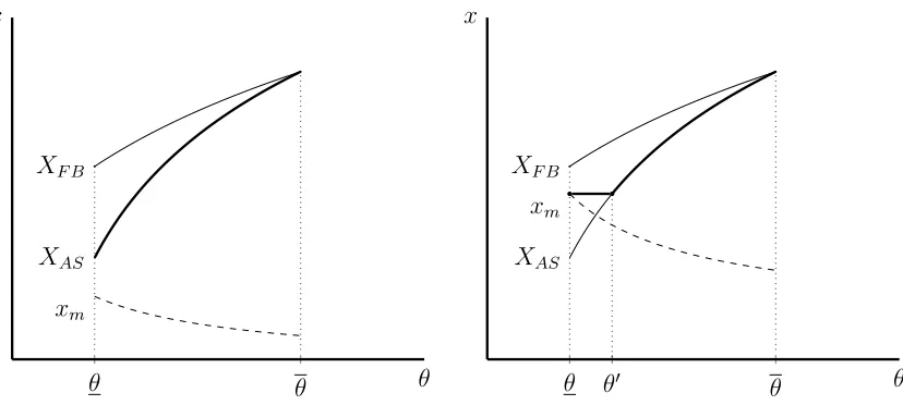
Proposition 4. If xm(θ) ≤ XF B(θ) then the optimal means of funding is a
pure grant for all types: V(θ) = 0 and G(θ)>0 for all θ. Moreover,
(1) If xm(θ)≤XAS(θ), then for all θ: X(θ) =XAS(θ), and G(θ) =GAS(θ).
(2) If XAS(θ)< xm(θ)≤XF B(θ), then there exists θ0 ∈(θ, θ) such that
(i) For θ∈[θ, θ0] there is bunching: X(θ) =G(θ) =x m(θ).
(ii) For θ ∈ (θ0, θ]: X(θ) = XAS(θ), G(θ) < X(θ) and 0 < G0(θ) <
X0(θ).
27G
✓ ✓ XF B
XAS
xm
✓ x
✓ ✓0 ✓
XF B
XAS
xm
✓ x
✓ ✓0 ✓00 ✓
XF B
XAS
xm
V
✓ x
✓ ✓
XF B
XAS
xm
V
✓ x
[image:23.612.117.531.110.296.2]1
Figure 1: Investment schedules (in bold) for the cases covered in Proposition 4. Case (1) is shown in the left panel, and case (2) in the right panel.
Proposition 4 reveals the circumstances in which optimal funding takes the form of a pure grant scheme, despite the MH problem. The optimal investment schedules for the two cases covered by Proposition 4 are shown in Figure 1.
Under the hypothesis of Proposition 4(1), XAS(θ) is sufficient to induce effort at each θ, i.e. xm(θ) ≤XAS(θ) for all θ. In this case, the MH problem is completely resolved – without a prize – at no additional cost to the funder. In the case covered by Proposition 4(2) there is an interval of low types such that for each θ in this interval, XAS(θ) is not sufficient to induce effort. For these types, the funder must raise investment aboveXAS(·), and/or offer a prize to elicit effort. Either way, greater rent will be generated for higher types. But there is an advantage to encouraging effort through greater investment. To see why, consider the problem of encouraging effort from a researcher of typeθ. Under the hypothesis of Proposition 4(2), XF B(θ) is sufficient to induce effort at θ, i.e., xm(θ) ≤ XF B(θ). As total surplus at any θ is strictly increasing in
the funder to the researcher. For this reason, effort is encouraged through increased investment, incentivized by a grant.
The discussion above suggests that whenever XAS(θ) < xm(θ) < XF B(θ) then it should be optimal for the funder to offer no prize, and specify the investment,xm(θ), to induce effort. However, xm(·) is strictly decreasing, and (IC-S) dictates that the investment schedule be non-decreasing when the prize is zero. Therefore, this investment schedule cannot be implemented over an interval of types, and bunching arises amongst low types.
The next result shows that if xm(θ) is larger than in Proposition 4, then a hybrid scheme is used for some types.
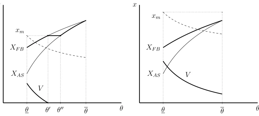
Proposition 5. If XF B(θ) < xm(θ) < XF B(θ) then the optimal means of
funding is a hybrid for sufficiently low types, and a pure grant for sufficiently high types. That is, G(θ) > 0 for all θ. While there is some θ0 ∈ (θ, θ) such
that if θ < θ0 then V(θ) > 0, and if θ ≥ θ0 then V(θ) = 0. Moreover, there
exists θ00∈(θ0, θ) such that,
(1) For θ∈[θ, θ0) investment is equal to the first-best, and is fully reimbursed
by the grant: X(θ) = G(θ) = XF B(θ).
(2) For θ∈[θ0, θ00] there is bunching: X(θ) =G(θ) = X
F B(θ0).
(3) For θ ∈ (θ00, θ]: X(θ) = XAS(θ), 0 < G(θ) < X(θ), and 0 < G0(θ) <
X0(θ).
The left panel of Figure 2 illustrates the prize and investment schedules for the case covered by Proposition 5. We first provide the intuition for the optimal hybrid scheme in the range of low types, [θ, θ0], given in Part (1).
✓ ✓ XF B
XAS
xm
✓ x
✓ ✓0 ✓
XF B
XAS
xm
✓ x
✓ ✓0 ✓00 ✓ XF B
XAS
xm
V
✓ x
✓ ✓
XF B
XAS
xm
V
✓ x
[image:25.612.120.534.110.296.2]1
Figure 2: Investment and prize schedules (in bold) for the cases covered in Proposition 5 (left panel) and Proposition 6 (right panel).
beyond first-best, as total surplus at any θ is strictly decreasing in x for x > XF B(θ). Instead, the funder sets investment equal to the first-best, X(θ) =
XF B(θ), and offers a prize,V(θ)>0, to induce effort.
To limit the researcher’s rent, the funder would like to keep the prize small. The smallest prize capable of eliciting effort from all types leaves (IC-E) bind-ing at each θ: θρ(x(θ))(v(θ) +π) = c. But for (IC-E) to bind over an interval of types, the term,ρ(x(·))(v(·)+π), must be strictly decreasing, which violates (IC-S). As a result, (IC-E) binds only at θ, and whenever V(θ) > 0, (IC-S) binds. To keep the prize as small as possible, a grant is used to fully offset the cost of investment. The optimal prize schedule, V(·), is the smallest prize consistent with IC that is capable of inducing effort from any type.
A researcher of type θ ∈ [θ, θ0] is indifferent between reporting her type truthfully, or any other ˆθ ∈[θ, θ0]. If, for instance, the researcher over reports, she receives a larger investment, which increases the likelihood of success, but she receives a smaller prize. In equilibrium, these two effects exactly offset.
that x(θ) ≥ XF B(θ0) > XAS(θ). For each type in this interval, the funder would like to reduce investment closer to max{XAS(θ), xm(θ)}, which is not feasible. Therefore, (IC-S) binds, and bunching arises.
Our final result in this section reveals conditions under which the optimal means of funding is a hybrid scheme for all types.
Proposition 6. If XF B(θ) ≤ xm(θ) then the optimal means of funding is a
hybrid for all types. Moreover, investment is equal to the first-best, and is fully reimbursed by the grant: V(θ) > 0 and X(θ) = G(θ) = XF B(θ) for all
θ ∈Θ.28
The intuition for the funding scheme outlined in Proposition 6 is similar to the intuition behind the hybrid scheme offered to low types in Proposition 5. The difference here is that the prize required to induce effort from the lowest type is large enough that, when combined with the bound on the slope ofV(·) provided by (IC-S), the prize is strictly positive for all types.
If one compares the optimal investment schedule under pure AS, XAS(·), with the optimal investment schedules characterized in Propositions 4-6, it is clear that for anyθ,XAS(θ)≤X(θ)≤XF B(θ). Thus total surplus is (weakly) higher at each θ when effort is unobservable, than when it is observable. The following corollary formalizes this observation.
Corollary 1. When the funder faces an AS problem, equilibrium total sur-plus is (weakly) higher at each θ when effort is unobservable, than when it is observable.
As mentioned in the introduction, in mixed models where the agent’s only action (effort) is unobservable and chosen after learning her type, effort tends to be distorted below the first-best to a greater extent than under pure AS. Corollary 1 shows that this is not the case when investment is observable. To understand the role played by the observable action, note that when actions are all unobservable, typically, the instruments that overcome MH also gener-ate significant rent for the agent (due to AS), and do not directly contribute to
28Proposition 6 also applies when lim
x→∞θρ(x)π < c, which means xm(θ) is not well
total surplus. For instance, if investment were unobservable in our model then greater investment/effort must be encouraged through a prize. The prize gen-erates significant rent for the researcher; to limit these rents, weaker incentives are provided, as compared to pure AS. In addition, the prize does not con-tribute to total surplus. As a result, total surplus is distorted further below the first-best, as compared to pure AS. In contrast, when investment is observable, it can be incentivized through the grant, and greater effort can be encouraged through the complementarity between the inputs. The grant is much more effective in limiting the researcher’s rent, and investment contributes directly to total surplus.
Let us make one remark as regards Corollary 1. We have assumed through-out that the funder finds it optimal to elicit effort from a researcher of any type. This assumption is more stringent in the model with combined AS and MH than with pure AS.29 If we relax this assumption, the welfare comparison
becomes less clear. Nevertheless, Corollary 1 provides a useful benchmark for comparing welfare when the social value of the project is sufficiently large.
Finally, Propositions 4 and 5 reveal that bunching may be a prominent feature of the optimal incentive scheme in our setting. In pure AS models, bunching is often avoided by assuming a monotone hazard rate (or inverse hazard rate) on the distribution over types. When bunching is not ruled out by this distributional assumption, frequently cited reasons for it to occur are countervailing incentives due to type-dependent outside options (see, e.g. Lewis and Sappington, 1989; Maggi and Rodriguez-Clare, 1995; Jullien, 2000), or “non-responsiveness” (see, e.g. Guesnerie and Laffont, 1984).30 In models
that combine AS and MH, bunching may arise for other reasons. Ollier and Thomas (2013) show that an ex post participation constraint may give rise to countervailing incentives, and bunching may occur for this reason. Gottlieb and Moreira (2015) show that bunching is a quite robust feature of binary
29i.e., If we relax this assumption, there may be instances where it is not optimal to elicit
effort from some low types under AS and MH, but where it is optimal to elicit effort from all types with pure AS.
30Non-responsiveness refers to a situation in which the first-best allocation is not
outcome models with AS, MH and limited liability. In our model, bunching does not arise for any of the reasons previously described; but rather, it is due to the conflict between rent extraction, effort inducement, and the second-order incentive compatibility constraint.
5
Discussion: The Use and Design of Push
Programs
When are push programs useful?
Proposition 4 shows that a pure grant scheme is optimal (for all types) in our model if xm(θ) ≤ XF B(θ). This condition provides insights into the cir-cumstances that a push program may be useful in practice. In particular, we conclude that a push program may be more relevant: (1) When AS is an issue; (2) For a more profitable project (i.e., π is large); (3) For a researcher with less valuable alternative endeavors, to which she can devote her time (i.e., the opportunity cost of effort, c, is small); (4) If there is a strong complementarity between capital and labor (i.e., p12(x, y) is large); and (5) For a project with
a high social value (i.e.,W +π is large).
Point (1) gives rise to the trade-off between a push and pull program. When AS is an issue, a pull program, while more effective in motivating un-observable effort, is a more expensive means of funding than a push program. Points (2)-(4) imply that the MH problem is not too severe, and that (less eas-ily observed) labor inputs (effort) can be encouraged through greater capital investments (which may be easier to verify). The intuition behind point (5) is the following:31 When MH is a concern, the funder must make the project
worth the researcher’s time. This may be done either through a prize, or if capital and labor are complements, through greater investment (incentivized via a grant). For a project with a high social value, the funder is willing to finance a greater investment, as doing so increases total surplus.
31Mathematically, point (5) holds since X
F B(θ) is positively related to both W and π,
These observations may help to shed light on patterns of funding observed in practice. Let us provide one concrete example. The Bill and Melinda Gates Foundation (GF) provides incentives for researchers to undertake projects re-lated to the development of pharmaceuticals used to treat/prevent certain dis-eases prevalent in the developing world. McCoy et al. (2009) offer a detailed report on the funding pattern of GF between 1998-2007. Over this period, it is reported that GF issued $8.95 billion in grants for global health. Of these funds, almost 37% were allocated to non governmental or non-profit research organizations, while less than 1% were awarded to for-profit firms.
Our results may help explain why GF uses a push program, and the distinc-tion it makes between non-profits and for-profits. First, AS is likely an issue, as expert researchers probably have better information than GF about the prospects of drug development. Second, for-profits and non-profits may differ in their natural motivations to undertake these projects. Due to a number of market failures, the profitability of these projects is low.32 A for-profit firm, if
motivated primarily by monetary incentives, would have little incentive to de-vote resources to these projects. A non-profit – setupspecifically to undertake these projects33– likely has other motivations (perhaps non-monetary). Third,
for-profits and non-profits may differ in the opportunity cost of devoting their time to these ventures: For-profits likely have other, more profitable ventures available, while this may be less of an issue for non-profits.34 Finally, these
projects are also of tremendous social value, as health and economic produc-tivity are intimately linked (see, e.g., Bleakley, 2010). Under these conditions, our model predicts that a push program may be optimal for motivating a non-profit, but it is less likely the case for a for-profit.
32See Kremer (2002) and Glennerster et al. (2006) for an overview of the issues
33The Program for Appropriate Technology in Health (PATH) is one example of this type
of non-profit (see, http://www.path.org/about/index.php). According to McCoy et al. (2009), PATH was awarded $949 million in grants from GF between 1998-2007.
34Some of these organizations, such as the Medicines for Malaria Venture, are setup
Design of push programs: R&D tax credits and matching grants
Our results also provide insights into the optimal design of push programs. One such program is the R&D tax credit system in the U.S. The U.S. Congress estimated that this system cost the federal government $6.9 billion in lost tax revenue 2013 (Hemel and Ouellette, 2013). In its simplest form, firms are awarded with a tax credit worth 20% of qualifying expenditures above some base amount. We show that the pure grant scheme characterized in Proposition 4(1) bears some semblance to this system.
Proposition 7. Under the hypotheses of Proposition 4(1), the optimal funding scheme can be implemented via a menu of linear contracts,{b(θ), r(θ)}θ∈Θ. For
each θ ∈Θ, the grant to the researcher takes the form,
˜
G(x, θ) =
0 x≤b(θ)
r(θ)(x−b(θ)) x≥b(θ)
where b0(·)>0, r(·)∈(0,1), r0(·)>0, and if c is sufficiently small, b(·)>0.
Proposition 7 reveals that the pure grant scheme can be implemented via a menu of linear contracts, {b(·), r(·)}, each of which specifies a base amount,
b(θ), and a reimbursement rate, r(θ). If the researcher selects {b(θ), r(θ)}, she is reimbursed nothing for each dollar she invests up to b(θ), and she is reimbursed at the rate of r(θ) per dollar she invests above b(θ). Higher types select higher base levels, and receive a greater rate of reimbursement.
Under the current system of R&D tax credits, a firm’s base amount is set according to past R&D expenditures. The logic is that the government would only like to reward firms for investment above and beyond what it would otherwise choose.35 Proposition 7 provides an alternative means to the same
end. Under our system, the researcher is free to choose her base amount, but she faces a trade-off between the base and the reimbursement rate.
Note that for a given base amount, b, and investment, x > b, the marginal value of an increase in the reimbursement rate isx−b. Therefore, the greater
the firm’s investment, the higher is the marginal value of an increase in the reimbursement rate. For this reason, a particularly productive firm (i.e., a highθ) that would like to invest more, is willing to accept a higher base, in ex-change for a higher reimbursement rate. In contrast to the current system, our system contemporaneously links the base amount to the firm’s desired invest-ment (rather than relying on past behavior), and provides stronger marginal incentives to more productive firms.
As mentioned in the introduction, one concern with the use of push pro-grams is that they may pay for research that is unlikely to succeed. Propo-sitions 3 and 4(1) shed light on this very issue. An important feature of the optimal funding scheme in these cases is that, while higher types receive larger grants, they are expected to bear a greater cost. In this way, only a researcher that is sufficiently likely to succeed is willing to receive a large grant. This feature of the funding scheme resembles a matching grant, which requires ex-penditures from the recipient in excess of the grant. Matching grants, and other cost-sharing programs, are commonly used by federal agencies in the U.S.36 Our results suggest that such schemes may be particularly effective in
dealing with AS.
Maurer and Scotchmer (2003) also point out that a matching grant can be an effective screening device in the presence of AS. Our results reveal the conditions under which this is in fact the optimal means of screening in a setting where MH is also relevant. Cost sharing policies have been advocated in other contexts for dealing with AS and MH. Laffont and Tirole (1986), for example, emphasize cost sharing as a way to elicit greater greater effort devoted to cost reduction, while still limiting the firm’s rent.
Capital constraints
One potentially important consideration for the form of funding, from which our model abstracts, is a capital constraint. Some push programs, such as research grants, provide upfront funding. It might be argued that this is
nec-36See
essary when the researcher has limited access to capital. As Scotchmer (2004, Ch. 8) also points out, this explanation is not satisfactory, as an appropriately designed pull program should be capable of attracting funding from financiers. Indeed, this is precisely the logic behind the “Pay for Success” model run by the U.S. Department of Labor (DOL).37It is also worth pointing out that other
push programs, such as R&D tax credits, do not provide funding upfront. Even so, while we do not include a capital constraint, our results may be useful for understanding the issue. Rather than an explicit inability to raise capital, one could alternatively imagine settings where (1) the socially-optimal level of investment is large; (2) the researcher has a strong incentive to devote her time and energy to a project; but (3) is unwilling to raise the necessary capital, given her costs and benefits. In our model, this translates to a setting whereXF B is large, πc is small, but the marginal cost of investment (normalized to 1) is large, relative to π. While a pull program could be used to encourage greater investment, our results imply that a push program may be optimal under these conditions.
6
Comparative Statics
This section compares the performance of grant and prize based funding when the strength of the MH problem increases. We then explore the relationship between the profitability of the project, and the optimal funding scheme.
From our results in Section 4.4, one may be tempted to draw the general conclusion that as the strength of the MH problem increases, a prize becomes
37According to DOL (https://www.doleta.gov/workforce_innovation/success.
cfm):
a relatively more attractive means of funding. As it happens, this conclusion is not precisely accurate in the context of our model. In fact, when the MH problem is weak, an increase in its severity (as measured by an increase in c) renders prizes, in some sense, less attractive to the funder.
In order to facilitate a comparison of grant and prize-based funding, sup-pose that the funder, for whatever reason, uses a pure prize scheme (i.e.
g(·) ≡ 0). Let φp(c) denote the funder’s optimal payoff when he encourages R&D activity using a pure prize, when the cost of effort isc. Letφg(c) denote the funder’s optimal payoff when he uses a pure grant scheme (i.e. v(·)≡ 0). Let D(c)≡ φg(c)−φp(c) denote the difference between the funder’s optimal pure-grant and pure-prize payoffs. Define the function ˜h as follows:
˜
h(θ) =
Rθ
θtf(t)dt
θ2f(θ)
For our next result, we assume that ˜h0(·)<0. Similar to the decreasing inverse hazard rate condition, this condition ensures full separation of types when the funder offers only a prize. This assumption is satisfied, for example, by a uniform distribution. We also assume that the researcher’s outside option is zero for each type: Π(θ) = 0 for allθ. Neither of these assumptions is necessary for the next result, but we impose them for ease of exposition.
Proposition 8. Assumeh˜0(·)<0, andΠ(θ) = 0 for allθ. Under the
hypothe-ses of Proposition 4(1), the difference between the funder’s optimal pure-grant and pure-prize payoffs, D(·), is strictly positive, and strictly increasing in c.
Proposition 8 shows that, in some sense, when the MH problem is weak, pure grant funding becomes relatively more attractive as the strength of the MH problem increases. To convey the intuition, suppose the effort cost in-creases slightly from c0 toc00 =c0+ ∆, but assume the hypotheses of Proposi-tion 4(1) are satisfied, for both costs. By ProposiProposi-tion 4(1), it follows that the optimal means of funding is the pure-grant scheme. Thus, D(·)>0.
the grant then increases by ∆ for each type θ > θ. Optimal investment, and the slope of the grant schedule, are unchanged. So following the cost increase, the researcher’s rent is unchanged, and the the funder’s payoff decreases by ∆. If the funder uses a pure-prize, the expected value of the prize offered to the lowest type increases by ∆ to maintain IR. However, when the prize offered to the lowest type increases, this creates a stronger incentive for higher types to underreport, and generates a greater rent for these types. To maintain IC, the expected value of the prize offered to all higher types increases by more than ∆. That is, the slope of the prize schedule increases. Therefore, the researcher’s expected rent increases, and the funder’s payoff decreases by more than ∆.
We now explore the comparative statics with respect to the profitability of the project, π. Since the optimal investment schedule under AS and MH is closely related to XAS(·) and XF B(·), we provide our comparative statics results with respect to these two functions. In what follows, we let φ∗ denote the funder’s ex-ante equilibrium expected payoff.
Proposition 9.
(i) For each θ ∈Θ, ∂XF B(θ)
∂π >0
(ii) ∂XAS(θ)
∂π >0 if and only if θ > h(θ)
(iii) ∂φ∂π∗ >0
An increase in π increases the total surplus generated in the event of suc-cess, and so it is intuitive that XF B(θ) is strictly increasing in π. But there are two competing forces acting onXAS(θ): On the one hand, the funder may want to increase XAS(θ) due to the increase in total surplus generated in the event of success. On the other hand, an increase in π increases the marginal cost of investment to the funder, due to the increased cost of maintaining IC.38
When θ > h(θ), the total surplus effect dominates the IC effect, andXAS(θ) increases in π (vice-versa when θ < h(θ)). Since θ > 0 = h(θ), investment
increases in π for sufficiently high types. Finally, part (iii) of Proposition 9 reveals that the funder is always better off (on average) when π increases.
Interestingly, the researcher’s equilibrium payoff may be either positively or negatively related toπ. The fact that the researcher’s payoff may be decreasing in the profitability of the project seems somewhat counterintuitive. To convey the idea, first note that the rent of a type-θ researcher is positively related to both π, and the investment of types just below θ. When an increase in π
leads the funder to reduce investment of some low types, the reduction in the researcher’s available rent may outweigh the gain in the available rent caused by the increase inπ. The following example illustrates; for the purposes of the example, we abstract away from MH, and set c= 0.
Example 1. Let c= 0, ρ(x) = 1−exp(−x), and θ ∼U1 4,1
. Using Propo-sition 4, V(θ) = 0, X(θ) = log(θ(W +π) −h(θ)π), where h(θ) = 1− θ. To calculate the researcher’s equilibrium payoff, u∗(θ), we plug X(·) into (3).
Suppose W = 6 and consider a slight increase in π from π = 1 to π = 1.05. Following the increase in π, the equilibrium investment and payoff of a type just aboveθ both decrease. For a researcher of type θ=.26, for example, X(θ)
decreases from about .07696 to .05449 and u∗(θ) decreases from about .00038
to .00015. The equilibrium investment and payoff of a high type both increase following the increase in π. Setting θ =.8, for example, X(θ) increases from about 1.6864 to 1.69194 and u∗(θ) increases from about .3392 to .35489.
One may also wonder whether more profitable projects should receive smaller or greater rewards from the funder. When V(θ)>0, it holds, G(θ) =
XF B(θ) and (as shown in the proof of Propositions 5 and 6)V(θ) = θρ(Xc
F B(θ))−
π. Following an increase inπ, XF B(θ) increases, so V(θ) decreases, and G(θ) increases.
forces on the grant related to IR. There is a direct effect: The project becomes more profitable, and hence, a smaller grant is required to ensure participation. But there is also an indirect effect: An increase in π may lead the funder to either increase or decrease investment (by Proposition 9(ii)). Ceteris paribus, an increase (decrease) in investment means a larger (smaller) grant is necessary to satisfy IR.
Similarly, following an increase in π there is a direct effect on IC: Ceteris paribus, an increase inπ generates greater information rent for the researcher, and a larger grant is used to maintain IC. But there is also an indirect effect since investment around some θ may increase or decrease. All else equal, an increase (decrease) in investment for types just below θ, increases (decreases) the rent of the typeθ, and increases (decreases) the size of the grant necessary to maintain IC. The net effect of a change in π on the grant depends on the balance of these forces and is, in general, ambiguous.
7
Conclusion
In this paper we fully characterized the optimal contracts in a setting where the inputs to production consist of both an observable and unobservable com-ponent, and the agent holds private information regarding the prospects of the project. We provided conditions under which pay-for-performance may not be optimal, and used our findings to shed light on push programs used in practice to encourage R&D. Although we focus on policy implications related to R&D funding, our model is useful for understanding the emergence of low-powered incentive schemes in many other contexts, e.g., worker compensation.
References
Baker, G. P. (1992). Incentive Contracts and Performance Measurement. Jour-nal of Political Economy, pages 598 – 614.
Basov, S. and Bardsley, P. (2005). A General Model of Coexisting Hidden Action and Hidden Information. Working paper No. 958, Department of Economics, University of Melbourne.
Bleakley, H. (2010). Malaria Eradication in the Americas: A Retrospective Analysis of Childhood Exposure. American Economic Journal: Applied Economics, 2(2):1–45.
Bolton, P. and Dewatripont, M. (2005). Contract Theory. MIT press.
Caillaud, B., Guesnerie, R., and Rey, P. (1992). Noisy Observation in Adverse Selection Models. The Review of Economic Studies, 59(3):595–615.
Chen, B. (2010). All-or-Nothing Monitoring: Comment. The American Eco-nomic Review, 100(1):625–627.
Chen, B. (2012). All-or-nothing payments. Journal of Mathematical Eco-nomics, 48(3):133–142.
Fu, Q., Lu, J., and Lu, Y. (2012). Incentivizing R&D: Prize or Subsidies?
International Journal of Industrial Organization, 30(1):67–79.
Glennerster, R., Kremer, M., and Williams, H. (2006). Creating Markets for Vaccines. Innovations, 1(1):67–79.
Gottlieb, D. and Moreira, H. (2015). Simple Contracts with Adverse Selection and Moral Hazard. The Wharton School Research Paper No. 78.