Accurate Gravitational Waveforms from Binary Black hole Systems

(1)

Accurate gravitational waveforms from binary

black-hole systems

Thesis by

Michael Boyle

in partial fulfillment of the requirements for the degree of

Doctor of Philosophy

California Institute of Technology Pasadena, California

2009

(2)

(3)

Come, you lost Atoms, to your Centre draw,

And be the Eternal Mirror that you saw:

Rays that have wander’d into Darkness wide,

Return, and back into your Sun subside.

From Farid ud-Din Attar’s twelfth-century masterpiece

(4)

(5)

Acknowledgments

My deep thanks go to Lee Lindblom, who has guided the first steps recounted herein with great patience and generosity. Kip Thorne has, when his busy sched-ule permitted, provided sage guidance and support, which have been crucial. Harald Pfeiffer and Mark Scheel have also been with me every step of the way, for which I am also very grateful. The four of them have lent their invaluable expertise to all my meanderings, and made sure I didn’t get too far off course—no small task.

Much of my education these past five years has also come from my fellow TAPIRs. All the grad students who have given talks at our weekly lunch meet-ings have broadened my knowledge of astrophysics. Everyone who has come to the relativity group meetings has added to my insight. My thanks to all of them. I especially thank Yanbei Chen, who has not only made group meetings more interesting, but has also sat on my candidacy and thesis committees. Alan Wein-stein also sat on both committees. I appreciate their efforts very much, because I’m sure it’s not the most entertaining or productive use of their time, though their presence certainly was beneficial to me.

I thank JoAnn Boyd whose capable guidance got me through all sorts of bureaucratic obstacles without a hitch, whose green thumb saved at least one very endangered shamrock plant, and whose friendship brightened my time in Pasadena.

Many other people have also made my time here much more enjoyable, doing

(6)

their best to distract me from the oppressive southern-California weather. Sherry Suyu brought me together with Ilya Mandel, Cynthia Chiang, and Luc Bouten for some excellent hot pot. Nate Bode, Geoffrey Lovelace, Rob Owen, Jon Pritchard, and Chris Wegg were friends first and fellow nerds second. Chang-Kook Oh provided much light-hearted relief from studying, along with the tastiest Korean food I’ve ever had.

My undergraduate experience at the University of Chicago was undoubtedly the most transformative period of my life (so far). Much of that was due to Arunas Liulevicius, whose profound understanding and enthusiastic teaching opened me up to the depths and beauties of rigorous thought. That eccentricity was successfully counterbalanced by Dietrich Müller and Simon Swordy, who brought me on surprisingly diverse explorations of a more sublunary realm by way of cosmic-ray detectors. Meanwhile, my close friends Sarah and Phil Barbeau, Baird Allis, John Allread, Dave Brick, Matt Keeshin, Jason Laine, and Ben Linford kept me sane and happy.

(7)

Abstract

We examine various topics involved in the creation of accurate theoretical gravi-tational waveforms from binary black-hole systems.

In Chapter 2 a pseudospectral numerical code is applied to a set of analytic or near-analytic solutions to Einstein’s equations which comprise a testbed for numerical-relativity codes. We then discuss methods for extracting gravitational-wave data from numerical simulations of black-hole binary systems, and intro-duce a practical technique for obtaining the asymptotic form of that data from finite simulation domains in Chapter 3. A formula is also developed to estimate the size of near-field effects from a compact binary. In Chapter 4 the extrapolated data is then compared to post-Newtonian (PN) approximations. We compare the phase and amplitude of the numerical waveform to a collection of Taylor approx-imants, cross-validating the numerical and PN waveforms, and investigating the regime of validity of the PN waveforms. Chapter 5 extends that comparison to include Padé and effective-one-body models, and investigates components of the PN models. In each case, a careful accounting is made of errors. Finally, we construct a long post-Newtonian–numerical hybrid waveform and evaluate the performance of LIGO’s current data-analysis methods with it. We suggest certain optimizations of those methods, including extending the range of template mass ratios to unphysical ranges for certain values of the total mass, and a simple an-alytic cutoff frequency for the templates which results in nearly optimal matches for both Initial and Advanced LIGO.

(8)

Acknowledgments v

Abstract vii

Contents viii

List of figures xi

List of tables xviii

1 Introduction 1

1.1 Generating gravitational waves . . . 2

1.2 Detecting gravitational waves . . . 5

1.3 Modeling gravitational waveforms . . . 7

1.4 This thesis . . . 9

2 Testing the numerical code 13 2.1 Introduction . . . 14

2.2 Solution method . . . 16

2.3 Random initial data on flat space . . . 22

2.4 Linear plane wave . . . 27

2.5 Gauge wave . . . 37

2.6 Gowdy spacetime . . . 48

2.7 Discussion . . . 52

(9)

Contents ix

3 Extrapolation 59

3.1 Introduction . . . 60

3.2 Extrapolation in brief . . . 66

3.3 Waveform extraction . . . 72

3.4 Extrapolation technique applied to binary inspiral waveforms . . . 80

3.5 Near-field effects in the data . . . 94

3.6 Conclusions . . . 108

4 Comparing NR to PN 111 4.1 Introduction . . . 112

4.2 Generation of numerical waveforms . . . 119

4.3 Generation of post-Newtonian waveforms . . . 160

4.4 PN–NR Comparison Procedure . . . 172

4.5 Estimation of uncertainties . . . 175

4.6 Results . . . 191

4.7 Conclusions . . . 212

5 Energy flux 217 5.1 Introduction . . . 218

5.2 Computation of the numerical gravitational-wave energy flux . . . 225

5.3 Post-Newtonian approximants . . . 235

5.4 Comparison with post-Newtonian approximants: Energy flux . . . 250

5.5 Estimation of (the derivative of) the center-of-mass energy . . . 266

5.6 Comparing waveforms . . . 271

(10)

5.8 Appendix: Padé approximants to the energy flux in the test particle

limit . . . 286

6 Data analysis 293 6.1 Introduction . . . 294

6.2 Searches for gravitational waves from black-hole binaries . . . 296

6.3 PN–NR hybrid waveform . . . 303

6.4 Detection efficiency of gravitational-wave templates . . . 313

6.5 Recommendations for improvements . . . 327

A Notation and conventions 335 A.1 Conventions in this thesis . . . 335

A.2 Comparison with other references . . . 344

B Spin-weighted spherical harmonics 347 B.1 Spin-weighted functions . . . 347

B.2 Behavior under rotation . . . 350

B.3 Multipole decompositions . . . 353

(11)

List of figures

2.1 Constraints for Minkowski space with random noise . . . 24

2.2 Error energy for Minkowski space with random noise . . . 26

2.3 Phase error for 1-D sinusoidal linear wave . . . 29

2.4 Constraints for 1-D Gaussian linear wave . . . 33

2.5 Error energy for 1-D Gaussian linear wave . . . 34

2.6 Constraints for 2-D linear waves . . . 38

2.7 Error energy for 2-D linear waves . . . 39

2.8 Constraints for high-amplitude 2-D gauge wave . . . 41

2.9 Error energy for high-amplitude 2-D gauge wave . . . 42

2.10 Constraints for shifted gauge wave . . . 46

2.11 Error energy for shifted gauge wave . . . 47

2.12 Constraints for expanding Gowdy spacetime . . . 50

2.13 Error energy for expanding Gowdy spacetime . . . 51

2.14 Constraints for collapsing Gowdy spacetime . . . 53

2.15 Error energy for collapsing Gowdy spacetime . . . 54

2.16 Comparing constraints for 1-D Gaussian linear waves . . . 56

3.1 Data-analysis mismatch between finite-radius waveforms and the ex-trapolated waveform for Initial LIGO . . . 63

3.2 Data-analysis mismatch between finite-radius waveforms and the ex-trapolated waveform for Advanced LIGO . . . 64

(12)

3.3 Convergence of the amplitude of the extrapolatedΨ4, with increasing order of the extrapolating polynomial, N . . . 84

3.4 Convergence of the phase of the extrapolatedΨ4, with increasing order of the extrapolating polynomial, N . . . 85 3.5 Convergence of the phase of Ψ4, extrapolated with no correction for

the dynamic lapse . . . 86 3.6 Convergence of the amplitude of the extrapolated h, with increasing

order of the extrapolating polynomial, N . . . 88

3.7 Convergence of the phase of the extrapolatedh, with increasing order of the extrapolating polynomial, N . . . 89 3.8 Comparison of extrapolation of Ψ4 using different sets of extraction

radii . . . 93 3.9 Relative amplitude difference betweenh data extracted at finite radius

and data extrapolated to infinity, and calculated near-field effects . . . 102

3.10 Phase difference between h data extracted at finite radius and data extrapolated to infinity, and calculated near-field effects . . . 103

3.11 Relative amplitude difference between Ψ4 data extracted at finite ra-dius and data extrapolated to infinity, and calculated near-field effects 106 3.12 Phase difference between Ψ4 data extracted at finite radius and data

extrapolated to infinity, and calculated near-field effects . . . 107

4.1 Eccentricity removal . . . 122

(13)

List of figures xiii

4.4 Deviation of total irreducible mass from its initial value . . . 132

4.5 Gravitational waveform extracted at r =240M . . . 135

4.6 Normalized constraint violations of run 30c-1 . . . 136

4.7 Unnormalized constraint violations of run 30c-1 . . . 137

4.8 Convergence of the gravitational-wave phase without time shifting . . 143

4.9 Convergence of the gravitational-wave phase with time shifting . . . . 144

4.10 Convergence of the gravitational-wave amplitude . . . 148

4.11 Convergence of the gravitational-wave amplitude . . . 149

4.12 Difference between areal radius rareal and coordinate radius r of se-lected extraction surfaces . . . 151

4.13 Convergence of phase extrapolation with extrapolating-polynomial order153 4.14 Convergence of extrapolated amplitude with extrapolating-polynomial order . . . 155

4.15 Effect of choice of wave-extraction radii on extrapolated phase . . . 156

4.16 Effect of choice of wave-extraction radii on extrapolated amplitude . . 157

4.17 Asymptotic behavior of the average lapse at large radii . . . 181

4.18 Asymptotic behavior of higher angular moments of the lapse at large radii . . . 182

4.19 Comparison of numerical simulation withTaylorT1 3.5/2.5waveforms— phase difference . . . 189

4.20 Comparison of numerical simulation withTaylorT1 3.5/2.5waveforms— relative amplitude difference . . . 190

(14)

4.22 Comparison of numerical simulation withTaylorT2 3.5/2.5waveforms—

phase difference . . . 193

4.28 Numerical and TaylorT4 3.5/3.0 waveforms . . . 204

4.29 TaylorT4 amplitude comparison for different PN orders . . . 205

4.30 Phase comparison for various PN approximants . . . 207

4.31 Late-time phase comparison for various PN approximants . . . 208

4.32 Phase differences between numerical and post-Newtonian waveforms at t=t(Mω=−0.063) . . . 210

4.33 Phase differences between numerical and post-Newtonian waveforms at t=t(Mω=−0.1) . . . 211

5.1 Some aspects of the numerical simulation . . . 224

5.2 Accuracy of the numerical flux . . . 230

(15)

List of figures xv

5.4 Accuracy of numerical $˙ . . . 233

5.5 Ratio of GW frequencies ω and $ to orbital frequency Ω . . . 252

5.6 Effect of choice of frequency type . . . 253

5.7 Comparison of NR and PN energy flux . . . 255

5.8 Early-time comparison of NR and PN energy flux . . . 256

5.9 Comparison of normalized energy fluxF/FNewt for equal-mass systems257 5.10 Cauchy convergence test of F/FNewt for T- and P-approximants . . . . 260

5.11 Fitting several PN approximants to the numerical flux . . . 262

5.12 GW frequency derivative$˙ for the numerical relativity simulation and various PN approximants at 3.5PN order . . . 265

5.13 Comparison of$˙ for the numerical results and various PN approximants267 5.14 Comparison of PN$˙ with a heavily smoothed version of the numerical ˙ $ . . . 269

5.15 Comparison of NR and PN dE/d$ versus GW frequency $ . . . 272

5.16 Phase differences between the numerical waveform, and untuned, orig-inal EOB, untuned Padé, and Taylor waveforms, at two selected times close to merger . . . 276

5.17 Phase differences between untuned and tuned P-approximants and NR waveforms . . . 278

5.18 Phase accuracy of various PN approximants . . . 281

5.19 Low-order normalized energy flux F/FNewt versus GW frequency 2Ω in the test-mass limit . . . 287

(16)

5.21 Convergence of the PN approximants in the test-mass limit . . . 289

5.22 Cauchy convergence test of F/F Newt in the test-mass limit for the

T-and P-approximants . . . 290

6.1 Convergence testing for numerical waveforms from a data-analysis per-spective . . . 306

6.2 Amplitude and phase differences between the numerical and post-Newtonian waveforms blended to create the hybrid waveform . . . 310

6.3 The last t=5000M_¯ of the hybrid waveform used in this analysis . . . 312 6.4 Hybrid Caltech–Cornell waveform scaled to various total masses shown

against the Initial- and Advanced-LIGO noise curves . . . 314

6.5 Histogram of overlaps found by 300 instances of the Amoeba algorithm316

6.6 Overlaps between Caltech–Cornell hybrid waveforms and restricted stationary-phase pN waveforms for the Initial-LIGO PSD . . . 320

6.7 Overlaps between Caltech–Cornell hybrid waveforms and restricted stationary-phase pN waveforms for the Advanced-LIGO PSD . . . 321

6.8 Integrand of the inner product for a TaylorF2 3.5 pN waveform . . . . 323

6.9 Overlap between Caltech–Cornell waveform and restricted TaylorF2, 3.5 pN waveform as a function of cutoff frequency fc . . . 325

6.10 Maximum overlaps obtained by allowing η to range over unphysical values, compared to those obtained by restricting the range of η . . . . 326

6.11 Candidate fc values for 3.5 pN templates with Initial LIGO . . . 329

(17)

List of figures xvii

(18)

4.1 Summary of the initial data sets . . . 121 4.2 Overview of low-eccentricity simulations . . . 128 4.3 Summary of uncertainties in the comparison between numerical

rela-tivity and post-Newtonian expansions . . . 177

5.1 Summary of PN approximants . . . 236 5.2 Normalized energy flux F/FNewt for the T- and P-approximants at

various PN orders and velocities vΩ . . . 258

5.3 Optimal a5 and vpole that minimize phase differences between tuned

EOB models and the numerical simulation . . . 280 5.4 Normalized energy flux F/F Newt in the test-mass limit for the T- and

P-approximants at different PN orders and at three different frequencies291

6.1 Maximum overlaps between Caltech–Cornell hybrid waveforms and restricted SPA pN templates using the Initial-LIGO noise curve . . . . 318 6.2 Maximum overlaps between Caltech–Cornell hybrid waveforms and

restricted SPA pN templates using the Advanced-LIGO noise curve . . 319

A.1 Comparison of sign conventions for geometric quantities. . . 346

(19)

C

hapter

1

Introduction

Down a quiet road in the woods of Louisiana, the darkness is warm and comforting. The sky is spread wide, bejeweled above a rippling wind sculp-ture, restless in the solitude. Nearby, on a few delicate fibers, hangs an almost flawless set of mirrors—virtually motionless. An intense beam of light shines across them. With sublime sensitivity, the light echoes out sounds of the dis-tant cosmos.

Almost a century ago, Einstein introduced an elegant theory to explain the nature of gravity. While the fundamentals are fairly simple and well understood, physicists have spent most of the past hundred years teasing out its implications. Gravitational waves, the Big Bang, and black holes—the broad strokes are all there; now we need to fill in the details. In recent years, we have begun to develop the tools that will allow us to investigate the most extreme environments in the universe. They will bring us deeper understanding of the theory’s consequences, and will be vital to the future of astronomy and physics.

Astronomy has always relied almost entirely on observations of light, pushing down to long-wavelength radio waves and up to high-energy gamma rays. A few

(20)

very interesting observations have also been made outside the electromagnetic spectrum, with neutrino telescopes and cosmic-ray detectors. As each new win-dow has opened, more unexpected phenomena have been discovered. Now, with gravitational waves, Einstein’s theory of general relativity is giving us a new way to extend our senses to the far reaches of the universe.

The signals, however, are extraordinarily subtle, squeezing and stretching the distance between objects near Earth by no more than a few parts in a billion bil-lion, and typically far less.1 Detecting them requires experiments of unsurpassed precision, and an accurate knowledge of just what the waves should look like. This thesis is an attempt to accurately model some of those waveforms. First, it will be helpful to review some of the most promising sources of gravitational radiation and the methods used to detect them.

1.1 Generating gravitational waves

Gravitational waves are ripples in the fabric of spacetime generated by acceler-ating masses. The greater the mass and the greater the acceleration, the larger the strain of the gravitational waves. Of course, like all radiation, the waves’ amplitudes fall off inversely with the distance r from the source. But simple acceleration is not sufficient. The source needs to have a changing quadrupole moment,2 the archetype of which is a simple binary—two bodies in orbit about each other. Indeed, the strongest astrophysical gravitational waves are expected

1_{The quantity used to measure the size of a gravitational wave is the}_strain_{, usually denoted}

(21)

1.1. Generating gravitational waves 3

to be produced by simple binaries.

If we denote the total mass of the system by M, the reduced mass by µ, and the orbital angular velocity by Ω, the typical strain produced by the wave is, in order of magnitude,

h≈ Gµ

c2_r

µ

GMΩ c3

¶_2/3

,

(1.1)

In terms of familiar scales, this is

h≈10−21 µ 1M_¯

1Mpc

r

µ

M

1M_¯

Ω 1Hz

¶_2/3

. (1.2)

The tiny coefficient gives us concern for the feasibility of detection. We need large masses, orbiting at high frequencies, as near to Earth as possible.

The closest contact binaries—pairs of more or less ordinary stars that are nearly touching—are found at roughly 100 pc from Earth, and orbit with periods as low as several hours [145]. If we assume typical masses of a few times the mass of the sun, this corresponds to a strain of about 10−20. In addition to concern for the minuscule magnitude of the strain, we need to worry about the frequency band in which it is found. On Earth, many things happen on timescales of several hours. Observing such tiny fluctuations without coupling to tides, or thermal cycling, or any number of vibrations is well beyond the capabilities of current earthbound technology, and even at the limit of expected capabilities of planned space-based detectors.

Ordinary stars undergoing fusion are simply too large and loosely bound to accelerate very quickly without breaking apart, which would tend to “smear out” the waves, reducing their strength. More compact objects are needed to produce

(22)

intense gravitational waves suitable for observations in the near future. White dwarfs, neutron stars, and black holes are the densest known concentrations of mass, and are known to be dynamic on timescales as brief as milliseconds [188]. This means that their frequencies can extend up to the kHz range,3 increasing the strain of the gravitational waves they emit, and placing those waves at frequencies that can be detected with high sensitivity.

Slightly elliptic spinning neutron stars would give off gravitational waves due to their changing nonsphericity. The waveforms emitted by such a star would be well modeled—basically a wave of constant frequency, modulated by the chang-ing orientation and velocity of the detector. Similar signals are likely given off by the neutron star of a low-mass X-ray binary [30]. The waves could be detected by demodulating the signal, taking its Fourier transform, and essentially looking for excess power [64].4 The longer the observation time, the more sensitivity there is to be gained. On the other hand, the fraction of the star’s mass involved in the type of nonsymmetric motion that gives off gravitational waves would be quite small, meaning that the waves themselves would be correspondingly small.

Alternatively, a close encounter between a pair of compact objects involves essentially all of the mass in nonsymmetric motion. We will see in Chapter 6 that, for merging nonspinning, equal-mass black-hole binaries, ³₁_MM_¯ _1HzΩ ´ reaches up to about 105. Thus, at its peak amplitude, the signal from such a binary will be

h≈10−18 µ 1M_¯

1Mpc

r . (1.3)

While this signal is indeed tiny for realistic masses and distances, it is nonetheless 3_{White-dwarf binaries would merge or break up at somewhat lower frequencies; this scale is} only valid for neutron stars and black holes.

(23)

1.2. Detecting gravitational waves 5

of a size that may be detected in the near future. The number of stellar-mass black holes in our galaxy is estimated to be in the hundreds of millions [193]. Though we have only a rough idea of how often these will meet and merge, it has been estimated that next-generation gravitational-wave detectors could detect merging black-hole binaries anywhere from dozens of times per year to a dozen times per day [102]. Even the lower number provides ample incentive to pursue detection of gravitational waves.

1.2 Detecting gravitational waves

Gravitational waves have been indirectly detected. Thirty years of observation of the binary pulsar B1913+16 have given us an accurate measurement of the system’s tightening [247]. The rate at which the binary inspirals agrees with the prediction for energy loss in the form of gravitational waves to within 0.2%. In 1993, the Nobel Prize was awarded to Hulse and Taylor for this observation. To date, however, no direct observation has been made.

(24)

the detection.

In interferometric detectors, there are three fundamental limiting sources of noise [155]:

• Seismic noise. This is filtered heavily through a system of coupled oscillators and active controls. It is dominant at low frequencies, dropping off very quickly at higher frequencies.

• Thermal noise. Produced by the suspension and within the mirror itself, the power in this noise source typically falls off roughly as f−4.5 _{and is} dominant just after the seismic noise drops off.

• Shot noise. This is noise due to photon counting statistics. Increasing with frequency, it takes over from thermal noise, and climbs as f2_.

Currently the most sensitive interferometers are the LIGO instruments.

With a low signal-to-noise ratio (SNR) it is simply not possible to just look at the data and see the signal. However, if we know what a possible signal would look like, we can test for its presence in the data. Though we can never be absolutely sure that a signal is or is not present, given a data stream s(t)

and a template waveformh(t), we can derive some likelihood statistic describing whether or not h is contained in s. This depends on the level of noise in the detector, Sn(f).6 We form the inner product

(s h)

B

4ℜ Z _∞

0

˜

s(f) ˜h∗(f)

Sn(f) df . (1.4)

(25)

1.3. Modeling gravitational waveforms 7

The larger this inner product is, the greater the likelihood that h is contained in s [65, 173], assuming the templates h are normalized to a constant. But this test assumes that we have a reasonably accurate template waveform h. If the template is inaccurate, it could match with noise just as well as it matches with the real data. Producing accurate waveforms and comparing them to models will be the main topic of this thesis.

1.3 Modeling gravitational waveforms

Science progresses by comparing its predictions to observations. General relativ-ity’s most intriguing results have only been encountered indirectly. Gravitational waves have been inferred to carry off energy from an inspiraling pair of stars. The existence of black holes has similarly been inferred from observations of the matter around them—evidence that so much mass is packed into such a small volume that we have no idea what might be in there other than a black hole. It would be comforting to have more direct observations, testing Einstein’s theory in the most severe environments in the universe today. Of course, to do that, we need to understand exactly what those predictions are.

To describe the motion of the Moon around the Earth to high accuracy, we only need Newtonian gravity. To describe the motion of Mercury around the Sun, we need a first-order approximation from Einstein’s theory [132]. The closer and more massive two orbiting objects are, the more we need general relativity. For a pair of black holes moving slowly, we can expand the terms in Einstein’s equations in series, and solve approximately. Techniques for doing these “post-Newtonian

(26)

approximations” have evolved over the past two decades, and have reached an impressive stage [42]. For some physical situations, they can accurately predict the waveform to within an orbit or two of the point of merger [59].7

However, as the black holes near each other, moving faster and faster, the ap-proximations must eventually break down. We have basically no hope of solving the full, nonlinear Einstein’s equations analytically. Instead, we need to use com-puters to simulate the physical scenario. While post-Newtonian approximations break down at some point before merger, numerical simulations are costly, and cannot extend for long before merger. We need to extend the simulations to a domain in which we trust the post-Newtonian approximations, and check that the predicted waveforms agree on the overlap. Then, the final waveform will be a marriage of post-Newtonian and numerical methods. In the following chapters we have done just this, demonstrating how to produce an accurate gravitational waveform for binary black holes.

Of course, it is entirely possible that exotic sources other than black-hole bi-naries exist, and will only be discovered through gravitational-wave astronomy— much as pulsars, active galactic nuclei, and the cosmic microwave background were only discovered with the advent of radio and microwave astronomy. One enticement to gravitational-wave astronomy is exploration of the unknown, as well as observation of the known. But the only way we will be able to discover new phenomena in the data will be to understand the more mundane signals— like binary black holes.

(27)

1.4. This thesis 9

1.4 This thesis

This thesis examines various topics involved in the creation of accurate theoretical gravitational waveforms from binary black-hole systems. The data presented is from a simulation of an equal-mass, nonspinning system, evolved through 15 orbits, merger, and ringdown. It is used to compare with post-Newtonian approximations, and to evaluate data-analysis techniques for gravitational-wave detectors.

In Chapter 2 we present tests of the numerical code used to evolve black-hole binary systems. The code is applied to a set of exact and approximate solutions to Einstein’s equations, which comprise a testbed for numerical-relativity codes— the so-called “Mexico City Tests”. While the formulation of Einstein’s equations is different from the one used to evolve binaries, the underlying code infrastructure and basic numerical methods are the same. This chapter is extracted with minor revisions from Ref. [62], and was written in collaboration with Lee Lindblom, Harald P. Pfeiffer, Mark A. Scheel, and Lawrence E. Kidder, and published in 2007.

(28)

courtesy of Mark A. Scheel, Harald P. Pfeiffer, and Luisa Buchman.

In Chapter 4 data extrapolated from a highly accurate 15-orbit simulation is then compared to post-Newtonian (PN) approximations. We compare the phase and amplitude of the numerical waveform to a collection of Taylor approximants, cross-validating the numerical and PN waveforms, and investigating the regime of validity of the PN waveforms. We find one particular approximant which agrees with our numerical waveform to within the uncertainty throughout most of the inspiral. This chapter is extracted with minor revisions from Ref. [59], which was written in collaboration with Duncan A. Brown, Lawrence E. Kidder, Abdul H. Mroué, Harald P. Pfeiffer, Mark A. Scheel, Gregory B. Cook, and Saul A. Teukolsky, and published in 2007.

Chapter 5 extends that comparison to include Padé and effective-one-body models, and investigates components of the PN models. In each case, a care-ful accounting is made of errors. The waveforms themselves are also compared, showing that Padé and EOB waveforms do have high accuracy, though only slightly better than the best Taylor approximant. This chapter is extracted with minor revisions from Ref. [61], which was written in collaboration with Alessan-dra Buonanno, Lawrence E. Kidder, Abdul H. Mroué, Yi Pan, Harald P. Pfeiffer, and Mark A. Scheel. It has been submitted to Physical Review D, and is under review.

(29)

1.4. This thesis 11

(30)

(31)

C

hapter

2

Testing the numerical-evolution code

1

The accuracy and stability of the Caltech-Cornell pseudospectral code is eval-uated using the Kidder, Scheel, and Teukolsky (KST) representation of the Einstein evolution equations. The basic “Mexico City Tests” widely adopted by the numerical-relativity community are adapted here for codes based on spectral methods. Exponential convergence of the spectral code is established, apparently limited only by numerical roundoff error or by truncation error in the time integration. A general expression for the growth of errors due to finite machine precision is derived, and it is shown that this limit is achieved here for the linear plane-wave test.

1_{This chapter is extracted with minor revisions from Ref. [62], which was written in} collabora-tion with Lee Lindblom, Harald Pfeiffer, Mark Scheel, and Larry Kidder. Note that the evolucollabora-tion system used in this chapter (KST) is not the same system used for the successful binary evolu-tions presented in other chapters (generalized harmonic). The code infrastructure, however, is the same. The code was written by Harald Pfeiffer, Mark Scheel, and Larry Kidder. I wrote the analytic solutions in the code (except for the linear wave), ran the simulations, and analyzed the data. Crucial suggestions to improve the parameters of the tests and refine the analysis came from all of my co-authors. I led the writing of most of the text, with some exceptions, though all authors contributed significantly. In particular, the introduction is due mostly to Lee Lindblom, Sec. 2.2 is due largely to Mark Scheel, and Sec. 2.7 was in large part written by Harald Pfeiffer.

(32)

2.1 Introduction

A number of groups have now developed numerical-relativity codes sophisticated enough to evolve binary black-hole spacetimes [219, 21, 81, 126, 158, 230]. The gravitational waveforms predicted by these evolutions will play an important role in detecting and interpreting the physical properties of the sources of these waves, soon to be detected (we anticipate) by the community of gravitational-wave ob-servers (e.g., LIGO, etc.). Therefore, such codes must be capable of performing stable and accurate simulations of very nonlinear and dynamical spacetimes.

(33)

2.1. Introduction 15

plane-wave initial data; (c) the evolution of a nonlinear gauge-wave representa-tion of flat spacetime; and (d) the evolurepresenta-tion of initial data for a very dynamic and nonlinear Gowdy cosmological model.

The Mexico City tests have now been applied to a number of different numerical-relativity codes that use different formulations of the Einstein equations [7, 17]. But all of the codes tested so far use finite-difference numerical methods. In this paper we report the results of applying these tests to the code developed in collaboration between the Caltech and Cornell numerical-relativity groups. We use a first-order symmetric-hyperbolic formulation of the equations developed by Kidder, Scheel, and Teukolsky [181] (sometimes referred to as the KST formula-tion) and we solve the equations using pseudospectral numerical methods. The results reported here differ therefore from all previously tested cases both in the formulation of the Einstein equations and the numerical methods used to solve them.

(34)

the stability of our evolution code for nonlinear gauge waves. In this case, nonlin-ear terms give rise to an instability that is drastically reduced by suitably filtering the components of the spectral expansion. Section 2.6 shows the performance of our code for evolutions of the highly dynamical Gowdy spacetime, in which the exact analytical expressions for the components of the fields grow exponentially in time. Finally, we discuss and summarize our various results in Sec. 2.7.

2.2 Solution method

In this section we describe the formulation of the Einstein equations and the pseudospectral numerical solution method that we test. The Mexico City tests were designed with finite-difference methods in mind and were originally ap-plied to formulations of the Einstein equations that are second-order in space and first-order in time. Both our numerical methods and our representation of the Einstein equations differ significantly from those in Ref. [7], so appropriate modifications to the Mexico City test suite (for example, the number of grid points used or the constraint quantities observed) are needed. These modifications are also described in this section.

2.2.1 KST formulation

(35)

2.2. Solution method 17

be put into first-order form. Its introduction results in two additional constraints:

Cki j

B

Dki j−1₂∂kgi j

,

(2.1)

Clki j

B

∂[lDk]i j . (2.2)

The KST evolution equations are obtained from the ADM equations [252] by adding constant multiples of the various constraints to the evolution equations and by replacing the lapse with a lapse-density function. These changes do not affect the physical solutions of the system, but they do modify the unphysical constraint-violating solutions. The added constraint terms are proportional to constant parameters ©γ1

,

γ2

,

γ3

,

γ4ª, which are chosen to make the system sym-metric hyperbolic [180]. The principal parts of the KST evolution equations, then, are given by:

∂tgi j 'Nn∂ngi j

;

(2.3)

∂tKi j 'Nn∂nKi j−N

h

(1+2γ0)gcdδn_(iδb_j)

−(1+γ2)gndδb_(iδc_j₎−(1−γ2)gbcδn_(iδd_j₎

+gnbδc_iδd_j+2γ1gn[bgd]cgi j

i

∂nDbcd

;

(2.4)

∂tDki j 'Nn∂nDki j−N

h

δn_kδb_iδc_j−1

2γ3gnbgk(iδcj)

−1

2γ4gnbgi jδck+ 1

2γ3gbcgk(iδnj)

+1

2γ4gbcgi jδnk i

∂nKbc . (2.5)

Here, the symbol ' indicates that terms algebraic in the fields (that is, nonprin-cipal terms) are not shown explicitly. The lapse function N is taken to be

(36)

and both the lapse density functionQ and the shift Ni are assumed to be speci-fied functions of the coordinates, rather than independent dynamical fields. Since each of the Mexico City tests involves reproducing either a known analytic solu-tion of the Einstein equasolu-tions or a small perturbasolu-tion about a known solusolu-tion, for all tests reported here we set the lapse densityQ and the shift Ni _{from the} appro-priate analytic solution. We choose one set of the KST parameters for all the tests here: γ0=0.5; γ1= −0.21232; γ2= −0.00787402; γ3= −1.61994; γ4= −0.69885. These values were chosen because they make the KST system symmetric hyper-bolic and coincide with a set preferred by Owen [204] in his extension of the KST system.

To evaluate errors it is useful to look at constraint quantities. As mentioned above, the KST system has additional constraints, Eqs. (2.1) and (2.2), besides the usual Hamiltonian constraintC and momentum constraintCi. To ensure that we are satisfying all the constraints, we monitor a single quantity C that is zero if and only if all of the constraints vanish:

C

B

q

C2₊₍_C_i₎2₊¡_C

ki j¢2+¡Clki j¢2

,

(2.7) where an object is squared using the evolved spatial metric. For example,(Ci)2=

gi j_C iCj.

Likewise, when evaluating differences from analytically known solutions, we define an overall error quantity that includes the errors in all evolved variables gi j, Ki j, and Dki j. Taking δgi j

B

g_{i j}analytic−g_{i j}evolved, and similarly for other

fundamental fields, this overall error quantity is given by

(37)

Note that δU vanishes if and only if all evolved variables match the known solution.

For all error quantities Q we display L2 norms:

kQk2

B

s

1

Vol

Z

Q2p_|_g_|_d3_x

_,

_(2.9)

where Vol=R p|g|d3x is the volume of the domain. These norms are computed after each time step over the current t=const. hypersurface. We refer to kCk2 as the constraint energy, and kδUk2 as the error energy.

The error quantities kδUk2 and kCk2 scale with the absolute magnitude of the fundamental fields and their derivatives, so it can be difficult to judge the significance of these error measures without knowing the overall scale of the variables in the problem. For this reason, we sometimes plot thenormalizederror energy kδUk2/kUk2 and the normalized constraint energy kCk2/k∂Uk2, where the normalization factors are defined by

U

B

q¡gi j¢2+¡Ki j¢2+¡Dki j¢2

,

(2.10)

∂U

B

q¡∂igjk¢2+¡∂iKjk¢2+¡∂iDjkl¢2 . (2.11)

(38)

perturba-tions of Minkowski spacetime, the overall scale is of order unity so it suffices to display the unnormalized quantities kδUk2 and kCk2.

2.2.2 Pseudospectral methods

All of our numerical computations are carried out using pseudospectral methods; this is the first time the Mexico City tests have been applied to a pseudospectral code. A brief outline of our method is as follows. Given a system of partial differential equations

∂tu(x

,

t)=F[u(x

,

t)

,

∂iu(x

,

t)]

,

(2.12)

where u is a collection of dynamical fields, the solution u(x

,

t) is expressed as a time-dependent linear combination of N spatial basis functions φk(x):

u(x

,

t)=

N_X−1

k=0

˜

uk(t)φk(x) . (2.13)

Associated with the basis functions is a set of Nc collocation points xi. Given spectral coefficientsu˜k(t), the function values at the collocation pointsu(xi

,

t)are computed using Eq. (2.13). Conversely, the spectral coefficients are obtained by the inverse transform

˜

uk(t)= NXc−1

i=0 wiu(

x_i

,

t)φ_k(x_i)

,

(2.14)

where wi are weights specific to the choice of basis functions and collocation points. Thus it is straightforward to transform between the spectral coefficients

˜

(39)

To solve the differential equations, we evaluate spatial derivatives analytically using the known derivatives of the basis functions,

∂iu(x

,

t)= N_X−1

k=0

˜

uk(t)∂iφk(x)

,

(2.15)

and we evaluate nonlinear terms using the values of u(x_i

,

t) at the collocation points. Thus we can write the partial differential equation, Eq. (2.12), as a set of ordinary differential equations for the function values at the collocation points,

∂tu(xi

,

t)=Gi[u(xj

,

t)]

,

(2.16) whereGi depends onu(xj

,

t)for all j. We then integrate this system of ordinary differential equations in time, using (for example) a fourth-order Runge-Kutta algorithm.

Because the tests discussed here are periodic in all spatial dimensions, we use Fourier basis functions. If we choose a computational domain extending from −1/2 to 1/2 in each of the x, y, and z directions, then each variable u is decomposed as

u(x

,

y

,

z)=NXx−1

k=0 N_Xy−1

l=0 NXz−1

m=0 aklmφk(x)φl(y)φm(z)

,

(2.17)

where

φk(x)=

              

1 k=0

;

sin[πx(k+1)] k>0 (k odd)

;

cos(πxk) k>0 (k even) .

(2.18)

(40)

pth-order finite differencing. As a result, we run our tests at coarser resolutions than those recommended in Ref. [7] for finite-difference codes—typically we use Ni =9, 15, 21, 27, and 33 collocation points in the relevant directions. From Eqs. (2.17) and (2.18) we see that if we choose Nx, Ny, or Nz to be an even in-teger, the highest-frequency component in our expansion will have a sine term but no matching cosine term. Consequently, the spatial derivative of this highest-frequency component will not be represented by our basis functions, causing a numerical instability. Therefore we choose Nx, Ny, and Nz to be odd.

Because spectral methods so greatly reduce spatial-discretization errors, time-stepping error is often dominant. In order to make the time time-stepping and the spatial-discretization errors comparable in these tests, we use fourth-order Runge-Kutta ODE integration. The time-step sizes are chosen in an effort to use step sizes comparable to those used to test finite-difference methods in Ref. [7], while also ensuring that time-step errors do not dominate over our spatial-truncation errors. We use ∆t =∆x/20 in the first test, and ∆t =∆x/40 in all others, except where explicitly noted. Here, ∆x is the minimum distance between collocation points.

2.3 Random initial data on flat space

(41)

2.3. Random initial data on flat space 23

noise to the initial data; the noise is intended to simulate the effect of finite numer-ical precision. A different random number is added to each component of each evolved variable, at each point in the domain. These random numbers are chosen to lie between −10−10 _and ₁₀−10 _{so that the system remains in the linear regime.} If these small perturbations to a simple spacetime grow unstably, it is likely that the inevitable errors (e.g., discretization error or even numerical-roundoff error) that arise in any more complicated simulation will also grow unstably. For this test we vary the resolution in the x dimension, and we fix the resolution to three collocation points in each of the y and z dimensions.

If the perturbations in the fields are chosen to be of size ², independent of resolution, then the perturbation in thenth spatial derivatives of these fields will be ∼²(∆x)−n_{, where} _∆_x _{is some measure of the distance between neighboring} points. This means that error quantities involving derivatives (such as constraints) will be larger for finer resolutions.2 This behavior is seen in the plot of the constraint energy in Fig. 2.1.

The purpose of this test is to establish that small constraint violations around flat space do not grow, and the KST system clearly passes this test. Whether or not constraint violations decay will depend on the evolution system and the numerical method. For example, artificial dissipation in the numerical method might cause all variations to decay, including constraint violations. Furthermore, 2_{The Mexico City collaboration [7] intended their Hamiltonian-constraint errors to be} inde-pendent of resolution, so they chose the size of the perturbation²to be dependenton resolution,

(42)

0 1×10−8 2×10−8 3×10−8

k

C

k2

0 250 500 750 1000

Crossing Times

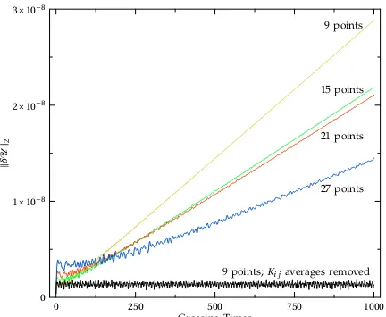
[image:42.612.76.503.179.537.2]

9 points 15 points 21 points 27 points

Figure 2.1: Constraints for Minkowski space with random noise

(43)

2.3. Random initial data on flat space 25

if the evolution system contains constraint damping in some form, then the con-straints should decay. Indeed, Owen has extended the KST system to include constraint damping [204]; running the same test, he observes exponential decay in the constraint quantities. The flat constraint violations observed in Fig. 2.1 in-dicate that the KST system with our parameter choice does not damp constraints and that the spectral method has insignificant artificial dissipation.

In Fig. 2.2 we see a linear growth of the error energy kδUk for this test. We find that the growth is caused solely by contributions from the metric gi j; the average values of Ki j and Dki j remain constant in time. We can understand this as follows. The average value of Ki j is determined by the random initial data and will in general be nonzero. The time derivative of Ki j, to first order in the amplitude of perturbations around flat space, involves only spatial derivatives of Dki j. (See Eq. (2.4).) These derivatives have zero average (up to roundoff errors

∼10−16), because the constant term in the Fourier expansion Eq. (2.18) is removed by differentiation, and therefore the average of Ki j will be constant in time. The time derivative of gi j involves a term proportional toKi j. Because the average of Ki j is constant in time and nonzero, the value of gi j will therefore drift linearly in time. The average ofKi j is smaller for higher resolutions—because the average is taken over more random numbers—which means that the growth rate of gi j should decrease with increasing resolution. Indeed, this is what we observe in Fig. 2.2.

(44)

0 1×10−8 2×10−8 3×10−8

k

δ

U

k2

0 250 500 750 1000

Crossing Times

[image:44.612.73.505.162.517.2]

9 points;Ki j averages removed 27 points 21 points 15 points 9 points

Figure 2.2: Error energy for Minkowski space with random noise

(45)

2.4. Linear plane wave 27

accomplished by setting the k=0 spectral coefficients of all components ofKi j to zero in the initial data, after all the random numbers have been added. The flat line in Fig. 2.2 shows the result, indicating that the average offset in Ki j is the only source of growth in the evolved variables of the KST system for this test.

2.4 Linear plane wave

If the ultimate goal of simulating binary black hole mergers is to predict the gravitational-radiation waveforms for observations, an evolution system must at least be capable of propagating a simple linear plane wave through flat spacetime. The form suggested for the Mexico City tests in Ref. [7] is

ds2= −dt2+dx2+(1+b)dy2+(1−b)dz2

,

(2.19)

where

b=b(x

,

t)=Asin[2π(x−t)] . (2.20) This metric satisfies Einstein’s equations only to linear order in the wave’s ampli-tude A, so if the fully nonlinear numerical solution is compared to this approx-imate solution, there will be deviations of order A2 _{that arise from our choice} of “analytic solution” rather than from numerical errors. The amplitude A for the Mexico City tests is chosen to be 10−8 so that such deviations in the metric components gi j are below machine precision. However, we still observe O(A2)

(46)

2.4.1 One-dimensional sinusoid

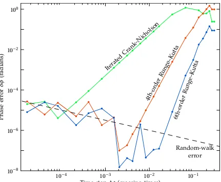
The sinusoidal waveform chosen in Eq. (2.20) is only a weak test for pseudospec-tral methods, because the Fourier basis functions defined in Eqs. (2.17) and (2.18) exactly resolve Eq. (2.20) at all times using only three basis functions; the only truncation errors are those associated with time discretization. Therefore, as a more challenging test, in Sec. 2.4.2 we repeat the plane wave evolution using a Gaussian-shaped wave. It is nevertheless instructive to evolve the sinusoid and study the resulting time-discretization errors. Since the dynamics involve no change in amplitude, but a change in phase, we expect the errors to be primarily phase errors, for reasonably small time steps.

This loss of temporal accuracy is particularly relevant in efforts to simulate sources for gravitational-wave observations, as the search for signals involves matching expected waveforms against observations. If there is significant error in the phase of the expected waveform, the overlap will be poor and detection will be more difficult. Although a constant overall scaling error in frequency—like the one found in this linear problem—could still result in detection, more complex situations would likely give rise to more complicated errors. The straightforward way to handle this problem is to minimize all time-stepping error.

In Fig. 2.3 we show the convergence of the phase error in the evolution of the sinusoidal linear wave. The solution is fully resolved on a3×1×1 grid. We keep this grid fixed, and decrease the size of the time step. Assuming that the only error is some phase error δφ, the evolved gzz will be given by

(47)

10−8 10−6 10−4 10−2 100

Phase

error

δφ

(r

adians)

10−4 ₁₀−3 ₁₀−2 ₁₀−1 Time step ∆t (crossing times)

Iterated Crank

–Nicholson

4th-or der

Rung e–K

utta

6th-or der

Rung e–K

utta

[image:47.612.111.542.161.517.2]

Random-walk error

Figure 2.3: Phase error for 1-D sinusoidal linear wave

(48)

At integer multiples of the light-crossing time for our computational domain, this can be written as

gzz=1−A£cosδφsin(2πx)+sinδφcos(2πx)¤ . (2.22) That is, we can find the phase error easily from the k=1 sine and cosine com-ponents of gzz (which happen to be easily accessible quantities in our code).

For intermediate time-step sizes, we can see convergence toward zero phase error with decreasing time step. As expected, we observe second-order conver-gence for Iterated Crank-Nicholson stepping, and fourth- and sixth-order for the appropriate higher-order Runge-Kutta algorithms. At very small time-step sizes, a new effect is seen, causing the phase error to increase with decreasing time step. This effect can be understood as machine-roundoff error accumulating via a random walk process.

Suppose we have a variable V(t) that is evolved by adding the small changes needed to update its value at each time step. Each such operation will introduce a fractional error χ(t) caused by the finite machine precision. We assume that the standard time-step size is∆t, and that there aren intermediate operations in each time step. After an evolution through time T, the total error added in this way will be

δV =n TX/∆t

j=0 V (tj)χ(tj) . (2.23)

To avoid tracking each individual error contribution, we treat χ as a random variable taking values in some range, with some probability distribution.

(49)

this accumulated error would be zero. Of course, we expect almost never to see this case: the most likely outcome is an accumulated error comparable to the dispersion:

|δV| ∼

q

(δV)2_∼sX j,k

V (tj)V(tk)χ(tj)χ(tk)

,

(2.24)

where the overbar indicates the average over the ensemble of random errors χ(t). We can simplify this expression by assuming that χ(t) has no correlations between time steps, and further assuming that the probability distribution is constant in time and uniform, taking values in the range [−²

,

²], where ² is the machine precision. This means thatχ(tj)χ(tk)=δjk²2/3. Finally, we approximate the discrete time sum as an integral, and obtain

|δV| ∼²

s

n

3∆t

Z _t₂

t1

V (t)2_dt _. _(2.25)

We can test this formula by observing its effects in the case of phase error for the linear wave. Here, the only nontrivial evolved variable is V =gzz, which is very nearly 1; so the integral in Eq. (2.25) becomes simply the evolution time T, which has the value25for the results plotted in Fig. 2.3. If phase errors dominate, δgxx∼Asinδφ, so we have

|δφ| ∼ ²

A

r 25n

3∆t ∼

10−7

p

∆t

³ _² 10−16

´µ₁₀−8 A

¶

,

(2.26)

(50)

The phase error is only so clearly visible in these evolutions because the full solution is described precisely at each moment by the first three basis functions. This means that discretization error due to spatial differentiation is essentially at the level of machine precision. Indeed, using more than three points actually degrades the quality of these one-dimensional sinusoid evolutions. Power in higher-order basis functions can only be error, and hence will necessarily do worse than the low-resolution case. We omit plots of the error energy and constraints in the higher-resolution cases, as they are very nearly the same as those of the more complicated two-dimensional evolutions discussed in Sec. 2.4.3.

2.4.2 One-dimensional Gaussian

As a more challenging test of pseudospectral methods, we repeat the one-dimensional linear wave test using a periodic Gaussian-shaped wave:

b=A X∞ j=−∞exp

"

−

¡

x−t+j¢2

2w2

#

,

(2.27)

(51)

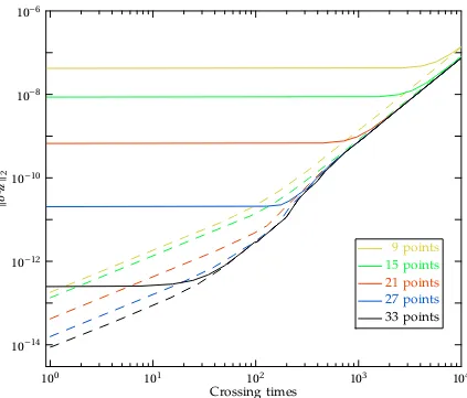
10−12 10−11 10−10 10−9 10−8 10−7

k

C

k2

0 2500 5000 7500

Crossing times

33 points

[image:51.612.112.541.156.534.2]

27 points 21 points 15 points 9 points

Figure 2.4: Constraints for 1-D Gaussian linear wave

(52)

10−14 10−12

10−10 10−8

10−6

k

δ

U

k2

100 101 102 103 104

Crossing times

9 points

15 points

[image:52.612.77.500.150.511.2]

21 points 27 points 33 points

Figure 2.5: Error energy for 1-D Gaussian linear wave

(53)

in Fig. 2.4. The constraint growth in the highest-resolution runs is slower than linear in time, and is probably caused by the accumulation of errors due to finite machine precision as discussed in Sec. 2.4.1.

Figure 2.5 presents the error energy for this run as the solid lines. At early times kδUk decreases exponentially to zero with increasing resolution, as one would expect. At late times, however, kδUk converges toward a parabola. The amplitude of this parabola scales in proportion to A2. In the rest of this section, we will first explain a subtlety arising when computing kδUk, followed by a detailed explanation of why the terms O(A2₎ _{manifest themselves in parabolic} behavior of kδUk.

The comparison of the computed solution with the analytic solution is per-formed at the collocation points. By virtue of the transformation Eqs. (2.13) and (2.14), the errors are initially exactly zero at the collocation points. The spatial-truncation error is nonzero of course, even at the initial time; it manifests itself as a deviation of the truncated series expansion from the analytic solution between collocation points. During the evolution, a linear wave will simply travel through the computational domain, returning to the original position after each light-crossing time. Since the spectral method has very small dispersion, the evolved shape remains the same. After each light-crossing time, therefore, the evolved solution again agrees to very high accuracy with the initial analytic solution at the collocation points. So, comparing the evolution with the analytic solution at integer multiples of the light-crossing time and at the collocation points will yield differences much smaller than spatial truncation error.3 Therefore, a fair

(54)

ison that includes the effects of spatial-truncation error must not be performed at integer light-crossing times. These considerations are evident from Fig. 2.5, where the solid lines show the “true” kδUk observed with 1/2 light-crossing interval offset, which suffices because the number of collocation points is always odd. The artificially small error energy observed at every complete light-crossing interval is shown as dashed lines, confirming the excellent low-dispersion property of our method.

At late times the differences between observation at full and 1/2 crossing times are swamped by the parabolic growth in kδUk. Similar parabolic deviations of the evolution from the solution of the linearized equations are observed for the other two linear-wave evolutions, the 1-D and 2-D sinusoids (see Fig. 2.7). The growth in kδUk appears almost entirely due to growth in the k =0 mode of diagonal terms inδgi j. Using evolutions of waves with different amplitudes and wavelengths, we have verified that this growth is proportional to A2t2/λ2, where A is the amplitude and λ the wavelength of the disturbance. The constant of proportionality depends directly on the KST parameter γ1 appearing in Eq. (2.4). This parameter controls the addition of a term γ1N gi jC to the ADM evolution equation for Ki j. The Hamiltonian constraint C is roughly constant in time, and varies as A2_/_λ2_{. Since the} _k₌₀ _{mode of} _γ

(55)

2.5. Gauge wave 37

2.4.3 Two-dimensional linear waves

The linear wave tests above may be modified by rotating the coordinates by π/4

about the z axis, which gives a plane wave propagating along the x-y diagonal. By increasing the size of the domain by a factor of p2 in each direction, the rotated solution can be made periodic while maintaining the same wavelength. This converts the spacetime from essentially one-dimensional to essentially two-dimensional. The purpose of this test is to ensure that the symmetry of the one-dimensional version does not hide sources of error (although propagation along a diagonal obviously retains some symmetries). For these tests we use a single collocation point in the z dimension, and we vary the (equal) number of collocation points in the x and y directions. We run these tests to t=1000—ten times longer than is recommended by the Apples with Apples collaboration—to better observe the stability properties. As shown in Fig. 2.6, the constraints for the sinusoidal wave increase with increasing x and y resolution (still using only a single point in the z direction). The constraints for the Gaussian are very nearly the same as in the one-dimensional case. Again, the A2_t2_/_λ2 _{growth of} _k_δ_U_k_is visible, as shown in Fig. 2.7.

2.5 Gauge wave

(56)

10−13 10−12

10−11 10−10 10−9 10−8

10−7

k

C

k2

0 200 400 600 800 1000

Crossing times

9 points

15 points

[image:56.612.74.503.157.521.2]

21 points 27 points

Figure 2.6: Constraints for 2-D linear waves

(57)

2.5. Gauge wave 39

10−13 10−12 10−11

10−10 10−9 10−8

10−7

k

δ

U

k2

101 102 103

Crossing times 9, 15, 21, and

27 points 27 points 21 points 15 points 9 points

Gaussian profiles Sinusoidal profiles

Figure 2.7: Error energy for 2-D linear waves

(58)

Mexico City test has the form

ds2= −(1+a)dt2+(1+a)dx2+dy2+dz2

,

(2.28)

a=Asin[2π(x−t)] . (2.29) Two cases are considered: a low-amplitude case with A=0.01, and a high am-plitude case with A=0.1. This is the first test for which the nonlinear terms in the equations play an important role.

For the linear plane wave test in Sec. 2.4, we found that because we use a Fourier basis, we were able to fully resolve the sinusoidal waveform using only three collocation points. This is not true for the gauge-wave test, because in this case the extrinsic curvature (one of our evolved variables) is not a simple sinusoid. Instead, its only nonzero component is

Kxx= −πpAcos[2π(x−t)]

1+Asin[2π(x−t)] . (2.30)

2.5.1 One-dimensional gauge wave

(59)

2.5. Gauge wave 41

10−16 10−12 10−8 10−4

100

k

C

k2

0 200 400 600 800 1000

Crossing times Unfiltered

Filtered

15 points

21 points

27 points 33 points

Figure 2.8: Constraints for high-amplitude 2-D gauge wave

(60)

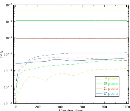
10−16 10−12 10−8 10−4

100

k

δ

U

k2

0 200 400 600 800 1000

Crossing times Unfiltered

Filtered

15 points

21 points

27 points 33 points

Figure 2.9: Error energy for high-amplitude 2-D gauge wave

(61)

2.5. Gauge wave 43

2.5.2 Two-dimensional gauge wave

A simple rotation of coordinates about the z axis makes the wave described by Eqs. (2.28) and (2.29) propagate along thex-y diagonal, as in the case of the linear wave. We use an equal number of collocation points in the x and y directions, and a single collocation point in z.

As for the one-dimensional gauge-wave test, we run at two different ampli-tudes: A=0.01 and A=0.1. For low amplitude, A=0.01, our evolution of the 2-D gauge wave is stable and convergent. Again, we omit plots, as our results are strictly better than for the more interesting high-amplitude case.

For high amplitude, A=0.1, we find an exponentially growing nonconvergent numerical instability, as seen in the curves labeled “unfiltered” in Figs. 2.8 and 2.9. This instability does not appear for the low-amplitude case, nor does it appear for either amplitude in the one-dimensional gauge-wave test.

The instability appears to be associated with aliasing caused by quadratic nonlinearities in the evolution equations; this is a well-known phenomenon that often occurs when applying spectral methods to nonlinear equations [58]. The basic mechanism for the instability can be understood by considering a truncated spectral expansion for some variable u(x) in terms of N basis functions φk(x):

u(x)=NX−1

k=0ukφk(x) . (2.31)

(62)

be simply discarded and the k<N coefficients should remain untouched. But it turns out that for the pseudospectral method of evaluating nonlinear terms (i.e., Fourier transform to obtain values at spatial collocation points, square these values, then Fourier transform back to spectral space), the power in the extra k≥N coefficients of the product does not disappear, but instead appears as ex-cess power in some of the k<N coefficients (“aliasing”). Repeating this process on each time step builds up this excess power and produces the instability.

Fortunately, there is a well-known remedy for instabilities caused by aliasing in nonlinear terms: suppose that the upper half (i.e., those with k≥N/2) of the coefficients uk in Eq. (2.31) were all zero. Then the spectral expansion of u(x)2 will have zeroes in all its k≥N coefficients, so there is no aliasing, and hence no instability. Therefore, we ensure that all coefficients with k≥kcut are zero by

removing those coefficients from the initial data and from the right-hand side of the evolution equations. It turns out (see, for example, Chapter 11.5 of Ref. [58]) that for a quadratic nonlinearity, it is sufficient to filter with kcut=2N/3 (and

not kcut=N/2) to eliminate aliasing. As mentioned in Sec. 2.2, the remaining

number of nonzero coefficients must be odd, which is ensured by reducing kcut

by one if necessary.

(63)

2.5. Gauge wave 45

from Figs. 2.8 and 2.9 that filtering dramatically reduces the instability. The initial constraint violations in these runs, kCk ≈10−12_{, are at the level of the finite} machine precision, so increasing the resolution causesincreased—not decreased— constraint violations.

2.5.3 Shifted gauge wave

We also show the results of a new “shifted gauge wave” test suggested for addi-tion to the “Apples with Apples” suite [17]. For this test we evolve flat space with the usual Minkowski coordinates (ˆt

,

xˆ

,

yˆ

,

zˆ) transformed to coordinates (t

,

x

,

y

,

z)

via

ˆ

t=t− A

4π cos[2π(x−t)]

,

(2.32) ˆ

x=x− A

4π cos[2π(x−t)]

,

(2.33) ˆ

y=y

,

(2.34)

ˆ

z=z . (2.35)

This test includes the effects of a nonvanishing shift vector. We use the same computational domain and KST parameters as in the standard gauge wave tests above. The amplitude suggested in Ref. [17] is A=0.5. We also run simulations with A=0.1.