The connected facility location polytope

The Connected Facility Location Polytope

Markus Leitnera_{, Ivana Ljubi´c}b_{, Juan-Jos´e Salazar-Gonz´alez}c_{, Markus Sinnl}a

a

Department of Statistics and Operations Research, University of Vienna, Austria

b

ESSEC Business School of Paris, France

c

DMEIO, Universidad de La Laguna, Tenerife, Spain

Abstract

We analyze the polytope associated with a combinatorial problem that combines

the Steiner tree problem and the uncapacitated facility location problem. The

problem, calledconnected facility location problem, is motivated by a real-world

application in the design of a telecommunication network, and concerns with

deciding the facilities to open, the assignment of customers to open facilities,

and the connection of the open facilities through a Steiner tree. Several solution

approaches are proposed in the literature, and the contribution of our work is a

polyhedral analysis for the problem. We compute the dimension of the polytope,

present valid inequalities, and analyze conditions for these inequalities to be

facet defining. Some inequalities are taken from the Steiner tree polytope and

the uncapacitated facility location polytope. Other inequalities are new.

Keywords: Valid inequalities, facets, facility location, Steiner trees

1. Introduction

This article concerns with the connected facility location problem (ConFL)

arising in the design of a telecommunication network. It is defined as follows.

LetI be the set of locations where a facility can be opened. LetJ be the set of customers. Each customer must be assigned to an open facility. LetK be the set ofintermediate nodes, i.e., locations that can be used for connecting open

Email addresses: [email protected](Markus Leitner),

[email protected] (Ivana Ljubi´c),[email protected](Juan-Jos´e Salazar-Gonz´alez),

facilities. All facility nodes can also be used for connection, regardless whether

they are opened or not. In telecom terminology, J represents terminals and S=I∪K representsSteiner nodes. The ConFL problem consists of selecting a subset ofI where facilities are opened, connecting these facilities through a tree structure that may use other Steiner nodes, and assigning the customers

to open facilities. There are costs associated with opening facilities, connecting

Steiner nodes, and assigning customers to facilities. The aim of ConFL is to

find a minimum-cost solution.

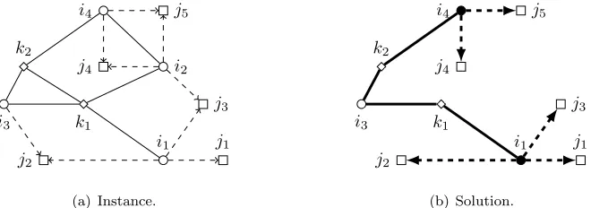
Figure 1(a) shows an instance of the problem and Figure 1(b) gives a feasible

solution. In the figure, I = {i1, . . . , i4}, J = {j1, . . . , j5} and K = {k1, k2}. Open facilities in the feasible solution are indicated in black. Note that in the

solution, facilityi3 is not opened, but it is used for the connection.

i1 i2

i3

i4

k1 k2

j1 j2

j3 j4

j5

(a) Instance.

i1

i2

i3

i4

k1 k2

j1 j2

j3 j4

j5

(b) Solution.

Figure 1: An instance of the ConFL problem in (a), and a feasible solution in (b).

The ConFL problem has been extensively addressed in the literature (see

e.g., [3, 4, 6, 7, 8, 9]), but all works concern solution approaches and computer

implementations. To our knowledge, this paper is the first investigation of the

ConFL polytope and it contributes to the literature with new inequalities.

Section 2 describes the notation that is used in this work. Section 3 computes

the dimension of the ConFL polytope. Section 4 adapts valid inequalities from

the literature, and Section 5 introduces new inequalities. In all cases, conditions

for the inequalities to define facets are investigated.

and presented in the “International Symposium on Combinatorial

Optimiza-tion” (Lisbon, 6-7 March 2014) [10].

2. Notation

Let G = (V, ES, AJ) be a mixed graph where V = S ∪J, the edge set

ES represents possible connections between Steiner nodes, and the arc set AJ

represents possible assignments of customers to facilities. In the context of

telecommunication, the edges represent the optical fiber cables in the core

net-work, and the arcs represent the copper cables connecting the customers to the

core network through servers. The graph (S, ES) is calledcore graph, and it is

assumed in this work to be complete, i.e.,ES ={{s1, s2}:s1∈S, s2∈S}. The

graph (I∪J, AJ) is calledassignment graph, and it is assumed to be complete

bipartite, i.e.,AJ ={(i, j) :i∈I, j∈J}. We also assume|I| ≥3 and|J| ≥3.

Finally, letc:ES∪AJ →R+0 andf :I→R+0 be given cost functions.

The ConFL problem can be modeled by using the following binary variables:

xe=

  

 

1 if edgeeis part of the solution

0 otherwise

fore∈ES;

ys=

  

 

1 if nodesis part of the solution

0 otherwise

fors∈S;

zi=

  

 

1 if facilityi is opened

0 otherwise

fori∈I;

aij =

  

 

1 if facilityiserves customerj in the solution

0 otherwise

fori∈I, j∈J.

For convenience of notation, we write (H :L) :={{s1, s2} ∈ES :s1 ∈H, s2∈

L} for H, L ⊂ S. For brevity, we write E(H) instead of (H : H) and δ(H) instead of (H :S\H). We also writex(F) :=P_e∈Fxe andy(H) :=Ps∈Hys

Using this notation, a formulation for the ConFL problem is:

min X

e∈ES

cexe+

X

i∈I

fizi+

X

(i,j)∈AJ

cijaij (1)

X

i∈I

aij = 1 ∀j∈J (2)

aij≤zi ∀i∈I,∀j∈J (3)

zi≤yi ∀i∈I (4)

x(E(S)) =y(S)−1 (5)

x(E(H))≤y(H)−ys ∀H⊂S,∀s∈H:|H| ≥2 (6)

(x, y, z, a)∈ {0,1}|ES|+|S|+|I|+|AJ| ₍₇₎

Constraints (2) force that every customer is assigned to a facility. Constraints

(3) ensure that a customer may be assigned to a facility when this facility is open.

Constraints (4) guarantee that a Steiner node with an open facility must be in

the solution. Constraints (6) are generalized subtour elimination constraints

and, together with (5), ensure that the solution is a tree in the core network

(see e.g. [13]). We will denote inequalities (6) as yGSECs and use (yGSEC) as

abbreviation for formulation (1)–(7).

We now analyze the polyhedral structure of the convex hull of the solutions

in (2)-(7). LetP be this polytope.

3. Dimension

The dimension ofP can be derived by using a lifting theorem based on the

dimensions of other known polytopes. Let S be the polytope of the spanning

treeproblem, U be the polytope of theuncapacitated facility location problem,

and Px,z,a

y (S′) = conv{(x, y, z, a) ∈ P : ys = 1,∀s ∈ S′} be an intermediate

polytope for S′ ⊆S. The projection of Px,z,a

y (S) on the x-space is S, and on

the (z, a)-space isU. SincePx,z,a

y (S) =S × {ys= 1,∀s∈S} × U, all facets of

S andU are also facets ofPx,z,a

y (S).

Starting from the dimension ofPx,z,a

y (S), we compute the dimension of the

Theorem 1. dim(Px,z,a

y (S)) =|ES| −1 +|AJ|+|I| − |J|.

Proof. The dimension ofS is|ES| −1 (see [2]) and the dimension ofU is|AJ|+

|I| − |J|(see [1]).

Theorem 2. For each S′⊆S,dim(Px,z,a

y (S′)) =|ES|+|S| −1 +|AJ|+|I| −

|J| − |S′|.

Proof. Clearlydim(Px,z,a

y (S′))≤ |ES|+|S| −1 +|AJ|+|I| − |J| − |S′| since

Px,z,a

y (S′)⊆R|E

S|+|S|+|AJ|+|I| _{and the |}

J| equalities (2), equality (5) and |S′|

equalitiesys= 1 are linearly independent. For the other direction, i.e., to prove

that dim(Px,z,a

y (S′))≥ |ES|+|S| −1 +|AJ|+|I| − |J| − |S′|, we claim that

there are|ES|+|S|+|AJ|+|I| − |J| − |S′|affinely independent solutions for a

givenS′_{. This is proven next by induction on the cardinality ofS\S}′_.

When|S′_{|=|S| the claim follows from Theorem 1. Suppose now that the} claim holds for a setS′with|S′|=ρand consider the setS′′=S′\ {s}for some s∈S′. By the induction hypothesis, there exist|ES|+|S|+|AJ|+|I| − |J| −ρ

affinely independent solutions, all withys= 1. To prove the claim, we need a

solution with ys= 0. This solution exits by the assumption that the instance

has at least two facilities and each facility is connected to all customers.

Corollary 1. dim(P) =|ES|+|S| −1 +|AJ|+|I| − |J|.

Theorem 2 forS′_{={s} proves the following result.}

Corollary 2. Inequalitiesys≤1 are facet-inducing forP for alls∈S.

4. Inequalities from the Uncapacitated Facility Location and

Span-ning Tree polytopes

The proof of Theorem 2 shows that every removal of a node fromSincreases the dimension ofPx,z,a

y (S) by one. Therefore the facets ofPyx,z,a(S) can be lifted

Lemma 1 ([12]). Let 1,2, . . . , u∈S. Let

X

e∈ES

αexe+

X

i∈I

δizi+

X

(i,j)∈AJ

ζijaij ≥η

be any facet-inducing inequality forPx,z,a

y (S). Then the lifted inequality

X

e∈ES

αexe+ u

X

s=1

βs(1−ys) +

X

i∈I

δizi+

X

(i,j)∈AJ

ζijaij ≥η

is valid and facet-defining forPx,z,a

y (S\ {1,2, . . . , u}), where

βs:=η−min

( X

e∈ES

αexe+ s−1

X

k=1

βk(1−yk) +

X

i∈I

δizi+

X

(i,j)∈AJ

ζijaij :

(x, y, z, a)∈ Px,z,a

y (S\ {1,2, . . . , s−1})andys= 0

)

for1≤s≤u.

The previous lemma allows us to obtain facets ofP from facets of the

unca-pacitated facility location polytopeU.

Theorem 3. The following inequalities are facet-inducing for P:

(a) aij ≤zi, for alli∈I andj∈J;

(b) aij ≥0, for alli∈Iandj ∈J;

(c) zi≤yi, for alli∈I.

Proof.

(a) The inequality induces a facet ofU, see [1]. Consider an arbitrary sequence

of S to lift theβ coefficients. For lifting node i, in any feasible solution,

zi = 0 when yi = 0 due to (4), and also aij = 0 due to (3). A feasible

solution exists since the core network is a complete graph and the customer

network is bipartite. Thus, we getβi= 0 as lifting coefficient. When lifting

nodeswiths6=i, one can either choose bothzi=aij = 1 orzi =aij = 0

(b) Everyaij ≥0 induces a facet ofU, see [1]. In an arbitrary lifting sequence,

for eachs∈S there is a solution withaij = 0, thusβs= 0.

(c) Every zi ≤1 induces a facet of U, see [1]. Consider an arbitrary lifting

sequence. When lifting nodei,zi= 0 due to (4) and thus we getβi=−1.

When lifting node s with s6= i there is a feasible solution with zi = 1,

thusβs= 0. We obtain−zi−(1−yi)≥ −1, which can be rewritten as

zi≤yi.

In a similar way, we can derive facet-inducing inequalities of P from the

spanning tree polytopeS.

Theorem 4. The following inequalities are facet-inducing for P:

(a) xe≥0, for all e∈ES;

(b)

x(E(H))≤y(H)−yu, (8)

for allH ⊂S:|H| ≥2,u∈H,|H∩I| ≤ |I| −1;

(c)

x(E(H))≤y(H)−1, (9)

for allH ⊂S:|H| ≥2,|H∩I|=|I|.

Proof.

(a) Everyxe≥0 induces a facet ofS, see [2]. Using the assumption that the

graphGis complete and|I| ≥3, there is a feasible solution of ConFL with xe= 0, no matter the lifting sequence ofS. Thenβs= 0 for alls∈S.

x(E(H)) =|H|−1. For eachs∈H\{u}, we getβs=−1 because the best

value forx(E(H)) is|H| −2. When lifting nodeu, we getβu= 0 because

there exists a feasible solution not using any node inH by connecting the customers to a facility outside H. Therefore in the lifting minimization problem x(E(H)) = 0 and P_s∈H\{u}βs(1−ys) = −|H|+ 1. Thus the

resulting facet-defining inequality is −x(E(H))−P_s∈H\{u}(1 −ys) ≥

−|H|+ 1, which can be rewritten asx(E(H))≤y(H)−yu.

(c) Similar to the (b), except in the last step, when lifting nodeu, there exists no feasible solution not using any node inH. This is because all facilities are inH. Thus, we getβu=−1 and therefore the resulting facet-defining

inequality is−x(E(H))−P_s∈H(1−ys)≥ −|H|+1, which can be rewritten

asx(E(H))≤y(H)−1.

Notice that we just proved that all the inequalities from the formulation (2)-(7)

are facet-inducing, except inequalities (6) for|H∩I|=|I|which are dominated by (9).

Finally, the uncapacitated facility location polytope suggests a new family

of facet-defining inequalities. Let us callinjective mapping a functionh:I→J such thath(i1)6=h(i2) wheni16=i2. Note that injective mappings exist when

|J| ≥ |I|.

Theorem 5. Let hbe an injective mapping. Then the inequality

X

i∈I

(zi+aih(i))≥2 (10)

is facet-inducing forP.

Proof. The inequality induces a facet ofU, see [5]. Consider an arbitrary lifting

sequence. Regardless of the lifted node s, the optimal objective value of the lifting problem is 2 because there is a solution where all customers are connected

5. New valid inequalities

We now present new valid inequalities for P and prove that some of them

are facets. All the proofs make use of a methodology calledindirect approach

which is based on the following result.

Lemma 2([12]). Let(A=_{, b}=_{)be the equality set ofP containingmequations,}

and letF={(x, y, z, a)∈ P:πxx+πyy+πzz+πaa=π0} be a proper face of

P. Then the following two statements are equivalent

1. F is a facet ofP

2. ifF ⊆ G ={(x, y, z, a)∈ P :αx+βy+γz+δa=λ0}then there exist some

s ∈ R and some t ∈ Rm_{, such that (α, β, γ, δ) = s(π}

x, πy, πz, πa) +tA=

andλ0=sπ0+tb=.

The equality set of the ConFL polytope P consists of (2) and (5), thus

m = |J|+ 1. In the proofs, we construct feasible solutions σ of the face F

under consideration, and evaluate them with the equality definingGin order to

determine the coefficients of this inequality. We denote byL(σ) the evaluation

ofαx+βy+γz+δaonσ. These evaluations will make clear the existence of somesandtas in the lemma, thus proving that F is a facet ofP.

5.1. aGSEC Inequalities

The first family of inequalities is motivated by the yGSECs (8), where the

node variable on the right hand side is replaced by a sum of assignment variables.

Theorem 6. Inequalities

x(E(H))≤y(H)− X

i∈I∩H

aij (11)

withH ⊂S: 2≤ |H| ≤ |I| −1, and j∈J are valid forP.

Proof. Note that P_i∈I∩Haij is at most 1 for any H due to constraints (2).

Moreover, the rhs is always larger than the associated left hand side (lhs) since

any feasible solution is always a tree due to constraints (5) and (6), and in any

(sub-)tree withnnodes there are at mostn−1 edges. Therefore, the inequality is valid forP.

Note that inequality (11) with|H∩I|=|I|is equivalent to the corresponding inequality (9) because of equations (2). Furthermore, inequality (11) withH∩

I={i}is dominated by the inequality (8) defined for H andi. For the special case when H = S \ {i} for some i ∈ I, the associated inequality (11) can be written as aij +x(δ(i)) ≥ yi. Finally, observe that the constraints (11)

suggest an alternative formulation for the ConFL problem, as they can replace

(6) in (1)–(7), leading to a model that we will refer to as (aGSEC) formulation.

Inequalities (11) will also be denoted as aGSECs in the following.

Theorem 7. Inequalities (11) are facet-inducing forP if and only if H ⊂S : 2≤ |H∩I| ≤ |I| −1.

Proof. LetF ={(x, y, z, a)∈ G: x(E(H))−y(H)−P_i∈I\Haij=−1}be the

proper face induced by (11) for somej∈J andH ⊂K: 2≤ |H∩I| ≤ |I| −1. Note that we have rewritten the inequality using equation (2) forj.

The feasible solutions σ ∈ F used in the proof are described by tuples Lq = (Sq∩H, Sq\H, Iq, Eq, Aq) where

• Sq ⊆S: core nodes involved in the solution (y-variables with value one);

• Iq ⊆I: open facilities in the solution (z-variables with value one);

• Eq ⊂ES: core edges in the solution (x-variables with value one);

• Aq ⊂AJ: assignment arcs in the solution (a-variables with value one).

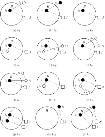
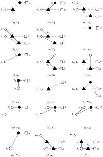
For eachi1, i2 ∈I; s1, s2 ∈ S; andJ′ := J \ {j}, the proof is based on a set of solutions depicted in Figure 2. In these figures, nodes inI,S andJ are represented by circles, diamonds and squares, respectively. Open facilities are

nodes from S) are drawn as diamonds. In addition, the proof also uses other solutions constructed by small modifications of the solutions listed below.

• L1= {i1},{i2},{i1},{{i1, i2}},(i1:J)

• L2= {i1},{i2},{i1, i2},{{i1, i2}},(i1:J)

• L3= {i1},∅,{i1},∅,(i1:J)

• L4= {i1, s1},∅,{i1},{{i1, s1}},(i1:J)

• L4′ = {i1, s1},{s2},{i1},{{i1, s1},{s1, s2}},(i1:J)

• L5= {i1},{s1, s2},{i1},{{i1, s1},{s1, s2}},(i1:J)

• L6= {i1},{s1, s2},{i1},{{i1, s2},{s1, s2}},(i1:J)

• L7= {i1, i2},∅,{i1},{{i1, i2}},(i1:J)

• L8= {i1, i2, s1},∅,{i1},{{i1, s1},{s1, i2}},(i1:J)

• L9= {i1, i2},∅,{i1, i2},{{i1, i2}},(i1:J′_{)∪ {(i2, j)}}

• L10= ∅,{i1},{i1},∅,(i1:J)

• L11= {i2},{i1},{i1, i2},{{i1, i2}},(i1:J′)∪ {(i2, j)}

ConsiderF ⊆ G and recall thatαrelates tox,β relates toy,γrelates to z, andδrelates toa. Then:

T7a γi= 0,∀i∈I:

To show that γi = 0 for i ∈ I\H, we compare the solutions L1 and

L2 (see Fig. 2(a) and 2(b)). Take any i2 ∈ I\H. The only difference between the two solutions is that inL1 facility i2 is closed, and inL2 it is open. SinceL(L1) =L(L2) thenγi2= 0.

To show that γi = 0 for i ∈ I∩H, we consider solutions L1′ and L2′,

H i1

i2

J

(a)L1

H i1

i2

J

(b)L2

H i1

J

(c) L3

H i1

s1 _J

(d)L4

H i1

s1

s2

J

(e)L_4′

H i1

s1

s2

J

(f)L5

H i1

s1

s2

J

(g)L6

H i1

i2 _J

(h)L7

H i1 s1

i2

J

(i) L8

H i1

i2 _J′

j

(j)L9

H

i1

J

(k)L10

H i2

i1

J′ j

(l)L11

Figure 2: Feasible solutions for the proof of Theorem 7

T7b αss′ =−β_s′,∀s∈H,∀s′∈S\H:

To show that αss′ = −βs′, ∀s ∈ H, s′ ∈ S \H, we compare the two

facility i1∈H, to which all customers are assigned to. Moreover, a core node s1 ∈ H is connected to i1. L4′ is nearly the same as L4, except

that there is an additional core node s2∈S\H, which is connected to s1. The result is obtained by considering L(L4) = L(L4′), which gives

αs1s2 +βs2 = 0 for s1 ∈ H, s2 ∈ S \H. Thus αss′ = −βs′ for all

s∈H, s′∈S\H.

T7c αss′ =−βs′,∀s, s′ ∈S\H:

Let L(L5′) be L5 without the node {s2} and edge {s1, s2}. The result

follows fromL(L5′) =L(L5), which givesα_s1s2+βs2= 0 fors1, s2∈S\H.

T7d βs=−α,¯ ∀s∈S\H:

L(L5) =L(L6), givesαi1s1 =αi1s2 fori1∈H, s1, s2∈S\H. Using the

results from step (T7b), we see that allβs,s∈S\H must have the same

coefficient, denote it by−α. Note that steps (T7c)-(T7d) are only needed¯ for|S\H| ≥2; otherwise, the result already follows from step (T7b).

T7e αss′ = ˆα,∀s, s′ ∈H and βs=−α,ˆ ∀s∈H:

First, suppose H ⊂I. L(L3) =L(L7) givesαi1i2+βi2 = 0 for i1, i2 ∈

H∩I. We can switchi1 andi2 in L3, L7and get αi1i2+βi1 = 0. Thus

αss′ =−β_s=−β_s′ fors, s′∈H∩I. Denote this value by ˆα.

Now, for |H\I|= 1, L(L3) = L(L4) implies αi1k1+βk1 = 0 for k1 ∈

H∩K, i1∈H∩I. Note that these coefficients are not yet related to ˆα. To determine the relation, considerL(L4) =L(L8). We get αk1i2 +βi2 = 0

fork1 ∈H∩K, i2 ∈H ∩I. Sinceβi2 =−αˆ we get αk1i2 = ˆα(and also

βk1 =−α). Thusˆ αss′ =−βs=−βs′ fors∈H∩I, s

′ _∈H.

Finally, for|H\I| ≥2 there are also coefficientsαss′ fors, s′∈H∩K. Let

L8′ beL8withk2∈H∩K instead ofi2∈H∩I. Then L(L4) =L(L8′)

givesαk1k2+βk2 = 0, from whichαss′ = ˆαfors, s

′ _{∈H∩Kfollows since}

βs′ =−α.ˆ

Let L7′ be L7 with i2 opened. From L(L7′) = L(L9), it follows that

δi1j=δi2j for alli1, i2∈H∩I. Denote this value by ¯δj.

T7g δij′ = ¯δj′, ∀i∈H∩I,∀j′ ∈J,j′6=j:

LetL9′ be L9 where customerj′, instead of customerj, is connected to

i2. FromL(L7′) =L(L9′) it follows thatδ_i1j′ =δi2j′ for alli1, i2∈H∩I,

j′_∈J,j′ _{6=j. Denote this value by ¯δ}

j′ forj′∈J,j′ 6=j.

T7h δij= ¯δj−αˆ+ ¯α,∀i∈I\H:

FromL(L10) =L(L11) we haveδi2j=βi1+αi1i2+δi1jfori2∈I\H, i1∈

H ∩I. Using results from steps (T7b), (T7d), (T7e) and (T7f), we get δij= ¯δj−αˆ+ ¯α, fori∈I\H.

T7i δij′ = ¯δj′, ∀i∈I\H,∀j′∈J,j′ 6=j:

Let L11′ be L11 where also customer j′ is connected to i2 instead of i1.

ThenL(L11) =L(L11′) givesδ_i2j′ =δi1j′ fori2∈I\H, i1∈H∩I. Using

the result from step (T7g), we getδij′ = ¯δj′ fori∈I\H.

T7j Defineρ:= ¯α−αˆ

Note that we can now write all coefficients in terms of ¯α, ρand ¯δj′ for j′ ∈J.

The equation definingG looks as follows:

(T7a)

z }| {

0z(I)−

(T7e),(T7j)

z }| {

(¯α−ρ)y(H)−

(T7d)

z }| {

¯

αy(S\H) +

(T7e),(T7j)

z }| {

(¯α−ρ)x(E(H)) +

(T7c),(T7d)

z }| {

¯

αx(E(S\H)) +

(T7b),(T7d)

z }| {

¯

αx(δ(H)) +

(T7f)

z }| {

¯ δj

X

i∈H∩I

aij+

(T7h),(T7j)

z }| {

(¯δj+ρ)

X

i∈I\H

aij+

(T7g),(T7i)

z _X }| {

j′∈J\{j} ¯ δj′

X

i∈I

aij′ =λ0.

By evaluating any feasible solution (e.g., L3) we get λ0 = L(L3) = ρ−α¯ +

P

j′∈Jδ¯j′. Rewriting the equation definingG, we get

−ρx(E(H))−y(H)− X

i∈I\H

aij

−α¯

(5)

z }| {

−x(E(S)) +y(S)+X

j′∈J

¯ δj′

(2)

z }| { X

i∈I

aij′

=ρ−α¯+X

j′∈J

Thus the equation definingGis a linear combination of the equation definingF

and the equality set ofP. Therefore, inequalities (11) are facet-inducing when

2≤ |H∩I| ≤ |I| −1.

To see that 2≤ |H∩I| ≤ |I| −1 is also a necessary condition, consider the following cases:

1. |H ∩I|= 0: Inequalities (11) reduce to x(E(H))≤y(H) and are domi-nated by inequalities (8).

2. |H∩I|= 1: Inequalities (11) reduce tox(E(H))≤y(H)−aij, withibeing

the unique facility inH. Thus they are also dominated by inequalities (8) sinceaij≤yi.

3. |H∩I|=|I|: Inequalities (11) are inequalities (9) (which are also facet-inducing).

5.2. Partition Inequalities

The following two families of inequalities are based on a partition of the

set of facilitiesI into two sets ˆI and I\I. The second family also involves aˆ partition of the setK of intermediate nodes. Moreover, both families also use an injective mappinghand assume that|K| ≥1.

The first family will be referred to as2+u partition inequalities, since, aside

from the partition of the facility set, a nodeu∈Kalso plays an important role in the definition of the inequalities.

Theorem 8. Let us consider u∈K,Iˆ⊂I and an injective mapping h. The inequality

X

i∈Iˆ

zi+

X

i∈I\Iˆ

(aih(i)+yi) +x( ˆI:K)≥1 +yu (12)

is valid forP.

Proof. If two (or more) facilities are opened, the inequality is clearly valid, since

y or a z variable on the lhs. Thus, we only need to concentrate on feasible solutions with one open facility. Three cases are possible:

(a) yu = 0: In a feasible solution, at least one facility must be opened and

thus the lhs is at least one.

(b) yu = 1: For this case, we make a further case distinction, depending on

whether the open facilityiis in ˆI orI\I:ˆ

• i∈I: Since both nodesˆ iand uare in the solution, there must be a connection betweeniandu. In this connection, there must either be an edge from some node in ˆI to a node in Kand thusx( ˆI :K)≥1, or an edge fromito a nodei′∈I\Iˆand thusyi′ = 1. Thus the lhs

of the inequality is at least two.

• i ∈I\I: As there is only one open facility, all customers must beˆ

connected toi, thusaih(i)must be one, and the lhs is at least two.

Theorem 9. Inequalities (12)are facet-inducing forP if and only if|I\Iˆ| ≥2

andIˆ6=∅.

Proof. Let

F={(x, y, z, a)∈ G:X

i∈_Iˆ zi+

X

i∈I\_Iˆ

(aih(i)+yi) +x( ˆI:K)−yu= 1}

be the proper face induced by (12) for someu∈Kand ˆI⊂I:|I\Iˆ| ≥2,Iˆ6=∅. The feasible solutionsσ ∈ F used in the proof are described by tuples Mq =

(Sq∩I, Sˆ q∩(I\I), Sˆ q∩K, Iq, Eq, Aq) where

• Sq ⊆S: core nodes involved in the solution (y-variables with value one);

• Iq ⊆I: open facilities in the solution (z-variables with value one);

• Eq ⊂ES: core edges in the solution (x-variables with value one);

Let K′ _{:= K\ {u}, J}′ _{:= J \ {j1}, J}′′ _{:= J \ {j2}. The following solutions,} wherei1, i4∈I;ˆ i2, i3∈I\I;ˆ k1∈K′_{,h(i2) :=j2,h(i3) :=j3, will be used. To} help a reader, the solutions are depicted in Figure 3. Facilities from ˆI andI\Iˆ are shown as circles and triangles, respectively. Open facilities are indicated in

bold. Intermediate nodes and sometimes also closed facilities (i.e., nodes from

S) are drawn as diamonds. Customers are shown as squares. In addition, some more solutions, which can be constructed by small modifications of the solutions

listed below, will also be used.

• M1= ({i1},{i2},{u},{i1, i2},{{i1, i2},{i2, u}},(i1:J))

• M2= ({i1},{i2},{u},{i1, i2},{{i1, i2},{i2, u}},(i1:J′_{)∪ {(i2, j1)})}

• M3= (∅,{i2, i3},{u},{i2, i3},{{i2, u},{i2, i3}},(i2:J′′_{)∪ {(i3, j2)})}

• M4= (∅,{i2, i3},{u},{i2, i3},{{i3, u},{i2, i3}},(i2:J′′_{)∪ {(i3, j2)})}

• M5= (∅,{i2, i3},{u},{i2, i3},{{i2, u},{i3, u}},(i2:J′′)∪ {(i3, j2)})

• M6= ({i1},∅,∅,{i1},∅,(i1:J))

• M7= ({i1},∅,{u},{i1},{{i1, u}},(i1:J))

• M8= ({i1},{i2, i3},{u},{i2, i3},{{i2, i1},{i2, i3},{i2, u}},(i2:J′′)∪{(i3, j2)})

• M9= ({i1},{i2, i3},{u},{i2, i3},{{i2, i1},{i1, i3},{i2, u}},(i2:J′′_{)∪{(i3, j2)})}

• M10= ({i1, i4},∅,∅,{i1},{{i1, i4}},(i1:J))

• M11= (∅,{i2},{u},{i2},{{i2, u}},(i2:J))

• M12= ({i1},{i2},{u},{i1, i2},{{i2, i1},{i2, u}},(i2:J′′)∪ {(i1, j2)})

• M13= ({i1},∅,{u, k1},{i1},{{i1, u},{u, k1}},(i1:J))

• M14= ({i1},∅,{u, k1},{i1},{{i1, k1},{u, k1}},(i1:J))

i1

i2 u

J

(a)M1

i1

i2 u

J′

j₁

(b)M2

i2

i3

u J′′

j2

(c)M3

i2

i3

u J′′

j2

(d)M4

i2

i3

u J′′

j2

(e) M5

i1 J

(f)M6

i1

u

J

(g)M7

i1

i2

i3

u J′′

j2

(h)M8

i1

i2

i3

u J′′

j2

(i)M9

i1

i4

J

(j)M10

i2 u

J

(k)M11

i1

i2

u J′′

j2

(l)M12

i1 u

k1 J

(m) M13

i1 u

k1 J

(n)M14

i2 u

k1 J

(o)M15

Figure 3: Feasible solutions for the proof of Theorem 9

Assume F ⊆ Gand recall thatαrelates tox,β relates to y, γrelates to z, andδrelates toa. Then:

T9a γi= 0,∀i∈I\I:ˆ

L(M1) =L(M1′).

T9b δij= ¯δj,∀j∈J,∀i∈I\Iˆ:h(i)6=j and∀i∈I:ˆ

L(M1) =L(M2) givesδi1j1=δi2j1, fori1∈I,ˆ i2∈I\Iˆand any customer

j16=h(i2). Since this step can be repeated for any facility inI, it follows that all coefficientsδijassociated with a customerj, except for the facility

i∈I\Iˆwithh(i) =j, have the same value. Denote this value by ¯δj.

T9c αii′ = ¯α,∀i, i′∈I\Iˆandαiu= ¯α,∀i∈I\I:ˆ

Obtained from L(M3) = L(M4) = L(M5), which gives αi2i3 = αi2u =

αi3u. Denote the value of the coefficients by ¯α.

T9d αiu=−βu,∀i∈I:ˆ

Obtained fromL(M6) =L(M7).

T9e αii′ = ¯α,∀i∈I\I,ˆ ∀i′∈Iˆandβi′ =−α,¯ ∀i′∈I:ˆ

L(M8) = L(M9) gives αi1i2 = αi2i3, for i2, i3 ∈ I \I,ˆ i1 ∈ I, thusˆ

αii′ = ¯α, using the result from step (T9c). The result βi′ =−α¯ follows

fromL(M8) =L(M3).

T9f αii′ = ¯α,∀i, i′∈I:ˆ

Obtained from L(M6) =L(M10), which gives αi1i2 =−βi2, ∀i1, i2 ∈I,ˆ

and the result follows from the result in step (T9e).

T9g δih(i)= ¯α+ ¯β+ ¯δh(i),∀i∈I\Iˆandβi= ¯β,∀i∈I\I:ˆ

FromL(M11) =L(M3), we getδi2h(i2)=αi2i3+βi3+δi3h(i2)fori2, i3∈

I\I. Using results from steps (T9b) and (T9c), we getˆ δi2h(i2) = ¯α+

βi3+ ¯δh(i2). Since this must hold for anyi3∈I\I, it follows thatˆ βi has

the same value for all i∈I\I. Denote this value by ¯ˆ β.

T9h Defineρ:= ¯α+ ¯β.

L(M12) =L(M8) givesγi1 =αi2i3+βi3, fori1∈I, i2, i3¯ ∈I\I, using theˆ

result from step (T9b). The resultγi=ρ,∀i∈I, is then obtained usingˆ

results from steps (T9c) and (T9g) and the definition from step (T9h).

T9j αiu= ¯α+ρ,∀i∈Iˆandβu=−(¯α+ρ):

L(M7) =L(M1) givesαi1u=αi2u+βi2+αi2i1 fori1∈I,ˆ i2∈I\I. Theˆ

resultαiu = ¯α+ρ,∀i∈I, follows from the results of steps (T9c), (T9e)ˆ

and (T9g) and the definition from step (T9h). The resultβu=−(¯α+ρ)

is then obtained using the result from step (T9d).

T9k αik= ¯α+ρ,∀i∈I,ˆ ∀k∈K′:

Obtained fromL(M13) =L(M14) using the result from step (T9j).

T9l αik= ¯α,∀k∈K′,∀i∈I\I,ˆ αuk = ¯α, ∀k∈K′ andβk=−α,¯ ∀k∈K′:

LetM11′ beM11 with the additional edge{u, k1}andM11′′ beM11with

the additional edge {i2, k1}. The result αik =αuk = ¯α is obtained by

L(M11′) = L(M11′′) = L(M15), using the result from step (T9c). The

resultβk =−α¯ is then obtained byL(M11′) =L(M11).

T9m αkk′ = ¯α,∀k, k′∈K′:

LetM15′ beM15with the additional edge{k1, k2}. We getαk1k2=−βk2

fork1, k2∈K′ and the result follows from the result in step (T9l).

Note that we can now write all coefficients in terms of ¯α, ρand ¯δj forj ∈J.

The equation definingG looks as follows:

(T9i)

z }| {

ρX

i∈_Iˆ zi+

(T9a)

z }| {

0 X

i∈I\_Iˆ zi−

(T9e)

z }| {

¯ αX

i∈_Iˆ yi+

(T9g),(T9h)

z }| {

(ρ−α)¯ X

i∈I\_Iˆ yi+

(T9c),(T9e),(T9f)

z }| {

¯

αx(E(I)) +

(T9j),(T9k)

z }| {

(ρ+ ¯α)x( ˆI:K) +

(T9c),(T9l)

z }| {

¯

αx(I\Iˆ:K) +

(T9j)

z }| {

(−ρ−α)y¯ u−

(T9l)

z }| {

¯ α X

k∈K′

yk+

(T9l),(T9m)

z }| {

¯

αx(E(K)) +

X

i∈I\Iˆ

(T9g),(T9h)

z }| {

(ρ+ ¯δh(i))aih(i)+

X

j∈J

(T9b)

z }| {

¯ δj

X

i∈I:h(i)6=j

By evaluating any feasible solution (e.g.,M6) we get

λ0=ρ−α¯+X

j∈J

¯ δj.

Rewriting the equation definingG, we get:

ρ X

i∈Iˆ

zi+

X

i∈I\Iˆ

(aih(i)+yi) +x( ˆI:K)−yu

−α¯

(5)

z }| {

−y(S) +x(E(S))+X

j∈J

¯ δj

(2)

z }| { X

i∈I

aij =ρ−α¯+

X

j∈J

¯ δj.

Thus the equation definingGis a linear combination of the equation definingF

and the equality set ofP. Therefore, inequalities (12) are facet-inducing, when

|I\Iˆ| ≥2,Iˆ6=∅.

To see that|I\Iˆ| ≥2 and ˆI6=∅ is also a necessary condition, consider the following cases:

1. ˆI=∅: Inequalities (12) reduce to

X

i∈I

(aih(i)+yi)≥1 +yu

and are dominated by inequalities (10).

2. |I\Iˆ|= 0: Inequalities (12) reduce to

X

i∈I

zi+x(I:K)≥1 +yu,

which are dominated by

X

i∈I

aij+x(I:K)≥1 +yu

for somej∈J. The latter inequalities are a combination of an equation (2) and an inequality

x(I:K)≥yu.

Rewrite this remaining inequality as

using equation (5). After further rewriting, we get

y(K′) +y(I)−1≥x(E(K)) +x(E(I)),

where K′ _{=K\ {u}. This inequality is easily seen to be a combination} of (6) and (9).

3. |I\Iˆ|= 1: LetI\Iˆ={i}. Inequalities (12) reduce to

X

i′∈I′

zi′+yi+aih(i)+x(I′ :K)≥1 +yu

forI′_{=I\ {i}. The inequalities are dominated by inequalities}

X

i′∈I

ai′h(i)+yi+x(I′:K)≥1 +yu,

which are a combination of an equation (2) and an inequality

yi+x(I′:K)≥yu.

Using equation (5), the latter inequality can be rewritten as

y(K′) +yi+y(I)−1≥x(E(K∪ {i})) +x(E(I))

where K′ =K\ {u}. Again, this inequality is easily seen to be a combi-nation of (6) and (9).

For the other new family of facet-inducing inequalities, consider also the

partition of the set of intermediate nodes K into three disjoint subsets K = K1∪K2∪K3, with|K1| ≥1. Before we present the inequalities themselves, we give two lemmas, which we will need for the validity proof of the inequalities.

Lemma 3. Let us consider K′⊆K. The inequality

x(K∪I:K′)≥y(K′). (13)

Proof. The inequalities are special case of constraints (9) forH =S\K′_{. This} can be verified as follows: Inequality (9) forH =S\K′_isx(E(S\K′_))≤y(S\ K′_{)−1. The result is obtained by rewriting this inequality using equation (5).}

Lemma 4. Let us consider Iˆ⊆I,u∈I\Iˆand an injective mapping h. The inequality

X

i∈_Iˆ zi+

X

i∈I\_Iˆ

(aih(i)+yi)≥1 +yu (14)

is valid forP.

Proof. For the case when z( ˆI)≥1, the inequality is obviously valid, so assume that z( ˆI) = 0. For somei ∈I\Iˆwe have yi = 1, thus the inequality is valid

ifyu = 0 . So, the only non-trivial case occurs when yu = 1, and yi = 0 for

all other nodesi∈I\I, iˆ =6 u. Since u∈I\Iˆis the only open facility, every customer has to be assigned tou. Thus auh(u)= 1 and therefore the left-hand side of the inequality is also equal to two, which concludes the proof. Note that

the proof also works for ˆI=∅.

Inequalities (14) are not facet inducing since they are dominated by

inequal-itiesz( ˆI) +y((I\I)ˆ \ {u}) +auh(u) ≥ 1, u ∈ I\I. These inequalities are inˆ turn dominated by inequalitiesz(I\ {u}) +auh(u) ≥1, u ∈ I\I. Finally, inˆ the latter inequalities, we can replace thez-variables with thea-variables going to customer h(u) and end up with P_i∈Iaih(u) ≥ 1, which is implied by the equation (2) from the formulation ofP, associated withh(u).

We are now ready to introduce the second family of facet-inducing

inequal-ities, which we will refer to as2+3 partition inequalities. The name indicates

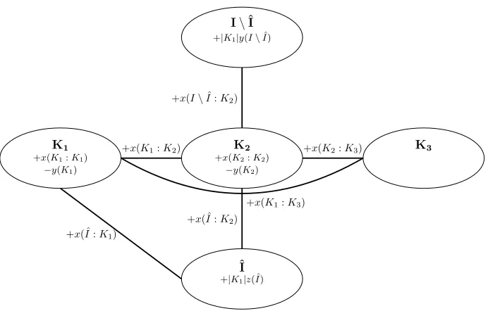
that the setsI andK are partitioned into two and three subsets, respectively. The variables associated with the core network, which occur in inequalities (15)

are illustrated in Figure 4.

K1

+x(K1:K1)

−y(K1)

K2

+x(K2:K2)

−y(K2)

K3

ˆI +|K1|z( ˆI)

I\ˆI +|K1|y(I\Iˆ)

+x(K1:K3)

+x(K2:K3)

+x(K1:K2)

+x(I\_Iˆ_:K2)

+x( ˆI:K1)

+x( ˆI:K2)

Figure 4: Illustration of the support graph of variables of the core network involved in

in-equalities (15), wherex₍K_:K1∪K2) =P2_i=1(x(Ki:Ki) +x(Ki:K3)).

and an injective mapping h. The inequality

|K1|X

i∈Iˆ

zi+|K1|

X

i∈I\Iˆ

(aih(i)+yi) +x( ˆI:K1∪K2) +x(I\Iˆ:K2)+

+x(K:K1∪K2)≥ |K1|+ X

k∈K1

yk+

X

k∈K2

yk (15)

is valid forP.

Proof. The proof is based on a connectivity argument: When some of the nodes

occurring on the rhs (i.e, nodes fromK1orK2) are in a solution, they must be connected to the rest of this solution. Thus also edges (which occur on the lhs

of the inequality) must be selected.

We make a case distinction depending on the value ofy(I\I).ˆ

• y(I\I) = 0 (i.e., no node fromˆ I\Iˆis in the solution):

remains to show thatx( ˆI :K1∪K2) +x(K :K1∪K2)≥y(K1) +y(K2) (note that opening more than one facility only increases the lhs and thus

it is enough to focus on the case, where z( ˆI) = 1). We can reformulate the lhs of the latter inequality asx( ˆI∪K:K1∪K2) =x(I∪K:K1∪K2) (since y(I\I) = 0), and so by Lemma 3, forˆ K′ _{=K1∪K2, the desired} result follows.

• y(I\I)ˆ ≥1: By Lemma 4, we have that z( ˆI) +P_i∈I\Iˆ(aih(i)+yi)≥2,

and therefore it only remains to show that x( ˆI : K1∪K2) +x(I\Iˆ : K2) +x(K:K1∪K2)≥y(K2). The latter inequality obviously holds by Lemma 3, forK′_=K2.

Observe that forK1 =∅, inequalities (15) only make sense for K2 6=∅. In this case, (15) reduce to the facet-inducing inequalities (9) forH=S\K2(shown in the form given in Lemma 3). The following theorem provides necessary and

sufficient conditions for these inequalities to be facet-inducing.

Theorem 11. Inequalities(15)are facet-inducing forP if and only if|I\Iˆ| ≥2

andIˆ6=∅.

Proof. Let

F={(x, y, z, a)∈ G:X

i∈Iˆ

zi+

X

i∈I\Iˆ

(aih(i)+yi)+

1

|K1|x( ˆI:K1∪K2)+

1

|K1|x(I\Iˆ:K2)+

+ 1

|K1|x(K1∪K2∪K3:K1∪K2)−

1

|K1| X

k∈K1

yk−

1

|K1| X

k∈K2

yk= 1}

be the proper face induced by (15) for some partition K = K1∪K2∪K3 :

|K1| ≥1 and ˆI⊂I :|I\Iˆ| ≥2,Iˆ6=∅. Note that we divided the inequality by

|K1|.

The feasible solutions σ ∈ F used in the proof are described by tuples

Nq= (Sq∩I, Sˆ q∩(I\I), Sˆ q∩K1, Sq∩K2, Sq∩K3, Iq, Eq, Aq) where

• Iq ⊆I: open facilities in the solution (z-variables with value one);

• Eq ⊂ES: core edges in the solution (x-variables with value one);

• Aq ⊂AJ: assignment arcs in the solution (a-variables with value one).

LetK₁′ =K1\{k1}, J′:=J\{j1}, J′′:=J\{j2}. The following solutions, where i1, i4 ∈I;ˆ i2, i3 ∈ I\I;ˆ k1 ∈K1, k2 ∈ K2, k3 ∈ K3, h(i2) := j2, h(i3) :=j3, will be used. To help a reader, the solutions are depicted in Figure 5. Nodes

fromK1,K2 andK3are shown as diamonds, pentagons and stars, respectively. Circles represent facilities and squares represent customers. Open facilities are

indicated in bold. In addition, other solutions, which can be constructed by

small modifications of the solutions listed below, will be used.

• N1= ({i1},{i2}, K1,∅,∅,{i1, i2},{{i1, i2}} ∪(i2:K1),(i1:J))

• N2= ({i1},{i2}, K1,∅,∅,{i1, i2},{{i1, i2}}∪(i2:K1),(i1:J′_{)∪{(i2, j1)})}

• N3= (∅,{i2, i3}, K1,∅,∅,{i2, i3},{{i2, i3}}∪(i2:K1),(i2:J′′)∪{(i3, j2)}) Note thatK1={k1} ∪K1′ as depicted in Figure (5(c)).

• N4= (∅,{i2, i3}, K1,∅,∅,{i2, i3},{{i3, k1},{i2, i3}} ∪(i2:K1′),(i2:J′′)∪

{(i3, j2)})

• N5= (∅,{i2, i3}, K1,∅,∅,{i2, i3},{{i2, k1},{i3, k1}} ∪(i2:K′

1),(i2:J′′)∪

{(i3, j2)})

• N6= ({i1},∅,∅,∅,∅,{i1},∅,(i1:J))

• N7= ({i1},∅,{k1},∅,∅,{i1},{(i1, k1)},(i1:J))

• N8 = ({i1},{i2, i3}, K1,∅,∅,{i2, i3},{{i2, i1},{i2, i3}} ∪(i2 : K1),(i2 :

J′′)∪ {(i3, j2)})

• N9 = ({i1},{i2, i3}, K1,∅,∅,{i2, i3},{{i2, i1},{i1, i3}} ∪(i2 : K1),(i2 :

J′′)∪ {(i3, j2)})

• N11= (∅,{i2}, K1,∅,∅,{i2},(i2:K1),(i2:J))

• N12= ({i1},{i2}, K1,∅,∅,{i1, i2},{{i2, i1}}∪(i2:K1),(i2:J′′_{)∪{(i1, j2)})}

• N13= ({i1},∅,{k1},{k2},∅,{i1},{{i1, k2},{k1, k2}},(i1:J))

• N14= ({i1},∅,{k1},{k2},∅,{i1},{{i1, k1},{i1, k2}},(i1:J))

• N15= ({i1},∅,{k1},{k2},∅,{i1},{{i1, k1},{k1, k2}},(i1:J))

• N16= ({i1},∅,∅,∅,{k3},{i1},{{i1, k3}},(i1:J))

• N17 = (∅,{i2, i3}, K1,∅,{k3},{i2, i3},{{i2, i3},{i2, k3}} ∪(i2 : K1),(i2 : J′′_{)∪ {(i3, j2)})}

• N18 = (∅,{i2, i3}, K1,∅,{k3},{i2, i3},{{i2, k3},{i3, k3}} ∪(i2 : K1),(i2 :

J′′)∪ {(i3, j2)})

We now supposeF ⊆ Gand determine the following properties of coefficients

ofG. Recall thatαrelates tox,β relates toy, γ relates toz, andδrelates to a. Note that some of the steps are almost similar to the previous proof.

T11a γi= 0,∀i∈I\I:ˆ

Let N1′ be N1, where facility i2 is not opened. The result follows from L(N1) = L(N1′). Note that if in the following steps, an open facility

i∈I\Iˆoccurs, we will not mentionγiexplicitly again, since the coefficient

is zero.

T11b δij= ¯δj,∀j∈J,∀i∈I\Iˆ:h(i)6=j and∀i∈I:ˆ

L(N1) =L(N2) givesδi1j1 =δi2j1, fori1∈I,ˆ i2∈I\Iˆand any customer

i16=h(i2). Since this step can be repeated for any facility inI, it follows, that all coefficientsδijassociated with a customerj, except for the facility

i∈I\Iˆwithh(i) =j, have the same value, denote it by ¯δj.

T11c αii′ = ¯α,∀i, i′∈I\Iˆandα_ik= ¯α,∀i∈I\I,ˆ ∀k∈K1:

Obtained from L(N3) = L(N4) = L(N5), which gives αi2i3 = αi2k1 =

i1

i2

K1

J

(a)N1

i1

i2

K1

J′

j1

(b)N2

i2

i3

K′

1

k1 J′′

j2

(c)N3

i2

i3

K′

1

k1 J′′

j2

(d)N4

i2

i3

K′

1

k1 J′′

j2

(e)N5

i1 J

(f)N6

i₁

k₁

J

(g)N7

i1

i2

i3

K1 J′′

j2

(h)N8

i1

i2

i3

K1 J′′

j2

(i)N9

i1

i4

J

(j)N10

i2

K1

J

(k)N11

i1

i2

K1 J′′

j2

(l)N12

i1

k1

k2 J

(m) N13

i1

k1

k2 J

(n)N14

i1

k1

k2 J

(o) N15

i1

k3

J

(p)N16

i2 i3 K1 k3 J′′ j2

(q) N17

i2 i3 K1 k3 J′′ j2

(r)N18

T11d αik= ˆα,∀i∈I,ˆ∀k∈K1,αkk′ = ˆα, ∀k, k′∈K1, andβ_k=−α,ˆ ∀k∈K1:

From L(N6) =L(N7), we getαi1k1 =−βk1, for i1 ∈I, k1ˆ ∈K1, which

means all coefficients for a particular k1 ∈ K1 are the same. Thus, if

|K1|= 1, we are already done. For |K1| ≥2, we also have edges αkk′:

Let N7′ be N7 with the additional edge {k1, k₁′} for k₁′ ∈ K₁′. From L(N7′) = L(N7), we get α_k1k′1 =−βk′1, fork1, k

′

1∈K1. It follows, that the coefficients αik, ∀i ∈ I,ˆ ∀k ∈ K1 and αkk′, ∀k, k′ ∈ K1 are all the

same, denote their value by ˆα. The result βk = −α,ˆ ∀k ∈ K1 follows

immediately.

T11e αii′ = ¯α,∀i∈I\I,ˆ ∀i′∈Iˆandβ_i′ =−α,¯ ∀i′∈I:ˆ

L(N8) = L(N9) gives αi1i2 = αi2i3, for ∀i2, i3 ∈ I\ I,ˆ i1 ∈ I, thusˆ

αii′ = ¯α, using the result from step (T11c). The resultβ_i′ =−α¯ follows

fromL(N8) =L(N3).

T11f αii′ = ¯α,∀i, i′∈I:ˆ

Obtained from L(N6) = L(N10), which gives αi1i2 = −βi2, ∀i1, i2 ∈ Iˆ

and the result follows from the result in step (T11e).

T11g δih(i)= ¯α+ ¯β+ ¯δh(i),∀i∈I\Iˆandβi= ¯β,∀i∈I\I:ˆ

From L(N11) =L(N3), we getδi2h(i2)=αi2i3+βi3+δi3h(i2)fori2, i3∈

I \I. Using results from steps (T11b) and (T11c), we getˆ δi2h(i2) =

¯

α+βi3+ ¯δh(i2). Since this must hold for anyi3∈I\I, it follows thatˆ βi

has the same value for alli∈I\I, denote it by ¯ˆ β.

T11h Defineρ:= ¯α+ ¯β.

T11i γi=ρ,∀i∈I:ˆ

L(N12) =L(N8) givesγi1 =αi2i3+βi3, fori1∈I, i2, i3¯ ∈I\I, using theˆ

result from step (T11b). The resultγi=ρ,∀i∈Iˆis then obtained using

results from steps (T11c) and (T11g) and the definition from step (T11h)

L(N7) =L(N1) givesαi1k1+βk1=

P

k∈K1αi2k+

P

k∈K1βu+βi2+αi2i1

fori1∈I,ˆ i2∈I\I. Using the results from steps (T11c), (T11d), (T11e), (T11g),ˆ (T11h), we get 0 =|K1|α¯−|K1|α+ρˆ and the result follows from rewriting this equation.

T11k αkk′ = ¯α+ _|Kρ

1|, ∀k ∈ K2,∀k

′ _{∈ K1,α}

ik = ¯α+ _|Kρ1|, ∀k ∈ K2,∀i ∈

ˆ I,

βk=−(¯α+_|Kρ1|),∀k∈K2:

The first two results are obtained fromL(N13) =L(N14) =L(N15), which

gives αk1k2 =αi1k1 =αi1k2 for i1 ∈ I, k1ˆ ∈ K1, k2 ∈K2 and using the

results from steps (T11d), (T11j). To get the resultβk =−

¯

α+_|Kρ_1|, letN14′ beN14without the edge{i1, k2}and nodek2. L(N14) =L(N14′)

which gives αi1k2 =−βk2 fori1∈I, k2ˆ ∈K2and the result follows.

T11l αik= ¯α+|Kρ1|,∀k∈K2,∀i∈I\

ˆ I:

LetN11′beN11with the additional nodek2and edge{i2, k2}fork2∈K2. L(N11) = L(N11′) gives α_i2k2 = −βk2 for i2 ∈ I\I, k2ˆ ∈ K2 and the

results follows by using the results from step (T11k).

T11m αkk′ = ¯α+_|Kρ

1|,∀k, k

′_∈K2:

LetN14′beN14with the additional nodek′₂and edge{k2, k₂′}fork′₂∈K2. L(N14) = L(N14′) gives α_k2k′2 = −βk′2 for k2, k

′

2 ∈ K2 and the results follows by using the results from step (T11k).

T11n αkk′ = ¯α+ ρ

|K1|,∀k∈K1,∀k

′_∈K3:

LetN16′beN16with the additional nodek1and edge{k3, k1}fork1∈K1. L(N16′) =L(N16) givesαk1k3=−βk1fork3∈K3, k1∈K1and the result

follows from using the results from steps (T11d), (T11j).

T11o αik= ¯α,∀k∈K3,∀i∈Iandβk=−α,¯ ∀k∈K3:

L(N17) =L(N18) givesαi2i3 =αi2k3 fori2, i3∈I\I, k3ˆ ∈K3. The first

∀k ∈ K3 follows. The first result, for the case i ∈I, then follows fromˆ

L(N6) =L(N16), which givesαi1k3 =−βk3 fori1∈I, k3ˆ ∈K3.

T11p αkk′ = ¯α+_|ρ

K1|,∀k∈K2,∀k

′_∈K3:

LetN16′′ be N16 with the additional nodek2 and edge{k3, k2} fork2∈

K2. L(N16′′) =L(N16) givesαk3k2 =−βk2 fork2∈K2, k3∈K3 and the

result follows by using the result from step (T11k).

T11q αkk′ = ¯α,∀k, k′∈K3: being a mammal (N) is necessary but not sufficient

to being human (S), Let N16′′′ be N16 with the additional nodek′₃ and

edge {k3, k′3} for k′3 ∈ K3. L(N16′′′) = L(N16) gives α_k3k′3 =−βk3 for

k3, k′

3∈K3and the result follows by using the result from step (T11o).

Note that we can now write all coefficients in terms of ¯α, ρand ¯δj, forj ∈J.

The equation definingG looks as follows:

(T11i)

z }| {

ρX

i∈Iˆ

zi+

(T11a)

z }| {

0 X

i∈I\Iˆ

zi−

(T11e)

z }| {

¯ αX

i∈Iˆ

yi+

(T11g),(T11h)

z }| {

(ρ−α)¯ X

i∈I\Iˆ

yi+

(T11c).(T11e),(T11f)

z }| {

¯

αx(E(I)) +

(T11d),(T11j)

z }| {

¯ α+ ρ

|K1|

x( ˆI :K1) +

(T11k)

z }| {

¯ α+ ρ

|K1|

x( ˆI:K2) +

(T11o)

z }| {

¯

αx( ˆI:K3) +

(T11c)

z }| {

¯

αx(I\Iˆ:K1) +

(T11l)

z }| {

¯ α+ ρ

|K1|

x(I\Iˆ:K2)

(T11o)

z }| {

¯

αx(I\Iˆ:K3) +

(T11d),(T11j)

z }| {

−α¯− ρ |K1|

X

k∈K1

yk+

(T11k)

z }| {

−α¯− ρ |K1|

X

k∈K2

yk−

(T11o)

z }| {

¯ α X

k∈K3

yk+

(T11d),(T11j)

z }| {

¯ α+ ρ

|K1|

x(E(K1)) +

(T11k)

z }| {

¯ α+ ρ

|K1|

x(K1:K2) +

(T11n)

z }| {

¯ α+ ρ

|K1|

x(K1:K3) +

(T11m)

z }| {

¯ α+ ρ

|K1|

x(E(K2)) +

(T11p)

z }| {

ˆ

αx(K2:K3) +

(T11q)

z }| {

¯

αx(E(K3)) +

X

i∈I\Iˆ

(T11g),(T11h)

z }| {

(ρ+ ¯δh(i))aih(i)+

X

j∈J

(T11b)

z }| {

¯ δj

X

i∈I:h(i)6=j

By evaluating any feasible solution (e.g.,N6) we get

λ0=ρ−α¯+X

j∈J

¯ δj.

Rewriting the equation definingG, we get:

ρ X

i∈Iˆ

zi+

X

i∈I\Iˆ

(aih(i)+yi) +

1

|K1|x( ˆI:K1∪K2) +

1

|K1|x(I\Iˆ:K2)+

+ 1

|K1|x(K1∪K2∪K3:K1∪K2)−

1

|K1| X

k∈K1

yk−

1

|K1| X

k∈K2

yk

−α¯

(5)

z }| {

(−y(S) +x(E(S))) +X

j∈J

¯ δj

(2)

z }| { X

i∈I

aij =ρ−α¯+

X

j∈J

¯ δj.

Thus the equation definingGis a linear combination of the equation definingF

and the equality set ofP. Therefore, inequalities (15) are facet-inducing, when

|I\Iˆ| ≥2,Iˆ6=∅, K16=∅.

To see that |I\Iˆ| ≥ 2,Iˆ 6= ∅ is also a necessary condition, consider the following cases:

1. ˆI=∅: Inequalities (15) reduce to

|K1|X

i∈I

(aih(i)+yi)+x(I:K2)+x(K:K1∪K2)≥ |K1|+

X

k∈K1

yk+

X

k∈K2

yk.

By Lemma 3 forK′=K2, we get

|K1|X

i∈I

(aih(i)+yi) +x(K\K2:K1)≥ |K1|+

X

k∈K1

yk.

Replace they-variables by thez-variables to obtain the stronger inequal-ities

|K1|X

i∈I

(aih(i)+zi) +x(K\K2:K1)≥ |K1|+

X

k∈K1

yk.

For the given injective mappingh, we now subtract inequalities (10)|K1|

times to obtain

x(K\K2:K1)≥ X

k∈K1

yk− |K1|.

This is obviously an aggregation of the upper bound inequalitiesyk ≤1 of

2. |I\Iˆ|= 0: Inequalities (15) reduce to

|K1|X

i∈I

zi+x(I:K1∪K2) +x(K:K1∪K2)≥ |K1|+

X

k∈K1

yk+

X

k∈K2

yk.

By Lemma 3 forK′=K1∪K2, we get

|K1|X

i∈I

zi ≥ |K1|.

Replace the z-variables bya-variables for some fixedj∈J. We get

|K1|X

i∈I

aij ≥ |K1|.

This inequality is easily seen to be implied by|K1|times the equation (2) for customerj.

3. |I\Iˆ|= 1: LetI\Iˆ={i}. Inequalities (15) reduce to

|K1|X

i′∈I′

zi′ +|K1|a_ih(i)+|K1|y_i+x(I′ :K1∪K2) +x(i:K2)+

x(K:K1∪K2)≥ |K1|+ X

k∈K1

yk+

X

k∈K2

yk

forI′=I\{i}. Replace|K1|yibyx(i:K1) to get the stronger inequalities

(sincexss′ ≤y_s due to inequalities (6) forH ={s, s′})

|K1|X

i′∈I′

zi′+|K1|a_ih(i)+x(I:K1∪K2)+x(K:K1∪K2)≥ |K1|+ X

k∈K1

yk+

X

k∈K2

yk.

By Lemma 3 forK′=K1∪K2, we get

|K1| X

i′∈I′

zi′+|K1|a_ih(i)≥ |K1|.

Replace the z-variables bya-variables forh(i)∈J. We get

|K1|X

i′_∈I

ai′_h(i)≥ |K1|.

Two special cases of inequalities (15) are of particular interest. One case

is given by the 2+2 partition inequalities that are obtained for K2 = ∅ and K3=∅. They are given as:

|K1|X

i∈Iˆ

zi+|K1|

X

i∈I\Iˆ

(aih(i)+yi)+x( ˆI:K1)+x(K:K1)≥ |K1|+

X

k∈K1

yk (16)

The other case is given by the2+1 partition inequalities that are obtained

forK2=∅andK3=∅(i.e.,K1=K). They are given as:

|K|X

i∈Iˆ

zi+|K|

X

i∈I\Iˆ

(aih(i)+yi) +x( ˆI:K) +x(E(K))≥ |K|+

X

k∈K

yk (17)

6. Conclusions

This article analyzes the polytope defined by the feasible solutions of the

connected facility location problem. This problem combines the uncapacitated

facility location problem and the Steiner tree problem, and has been motivated

by a telecommunication application. The article computes the dimension of

the polytope and shows several families of valid inequalities. Some of these

inequalities are lifted variants from the uncapacitated facility location polytope.

Other inequalities are taken from the polytope of the Spanning Tree problem.

In addition, the article also presents new inequalities exploiting the interaction

of the two combinatorial structures, like what we call partition inequalities. The

article also study conditions under which these inequalities are facet defining.

The proofs are based on the so-called indirect method. Some of the inequalities

analyzed in this article are used in [11] to describe a branch-and-cut approach

to design telecommunication networks with a tree-star topology.

Acknowledgements

This work is supported by the Vienna Science and Technology Fund (WWTF)

through project ICT15-014. M. Leitner, I. Ljubi´c, and M. Sinnl are supported

by the Austrian Research Fund (FWF) under grants I892-N23 and

P26755-N19. J.J. Salazar-Gonz´alez is supported by the Spanish Government through

References

[1] G. Cornuejols and J.-M. Thizy. Some facets of the simple plant location

polytope. Math. Programming, 23(1):50–74, 1982.

[2] J. Edmonds. Submodular functions, matroids, and certain polyhedra.

Com-binatorial structures and their applications, pages 69–87, 1970.

[3] S. Gollowitzer and I. Ljubi´c. MIP models for connected facility location:

A theoretical and computational study. Comput. & Oper. Res., 38(2):435–

449, 2011.

[4] F. Grandoni and T. Rothvoß. Approximation algorithms for single and

multi-commodity connected facility location. In O. G¨unl¨uk and G.

Woeg-inger, editors,IPCO 2011, New York, NY, USA, Proceedings, volume 6655

ofLNCS, pages 248–260. Springer, 2011.

[5] M. Guignard. Fractional vertices, cuts and facets of the simple plant

lo-cation problem. In M. Padberg, editor, Combinatorial Optimization,

vol-ume 12 of Mathematical Programming Studies, pages 150–162. Springer

Berlin Heidelberg, 1980.

[6] F. Havet and M. Wennink. The push tree problem. Networks, 44(4):281–

291, 2004.

[7] D. Karger and M. Minkoff. Building Steiner trees with incomplete global

knowledge. InFOCS, pages 613–623. IEEE Computer Society, 2000.

[8] C. Krick, H. R¨acke, and M. Westermann. Approximation algorithms for

data management in networks.Theory Comput. Syst., 36(5):497–519, 2003.

[9] M. Leitner and G. R. Raidl. Branch-and-cut-and-price for capacitated

connected facility location. J. of Math. Modelling and Algorithms, 10(3):

[10] M. Leitner, I. Ljubi´c, J. J. Salazar-Gonz´alez, and M. Sinnl. On the

asym-metric connected facility location polytope. Lecture Notes in Computer

Science, 8596:371–383, 2014.

[11] M. Leitner, I. Ljubi´c, J. J. Salazar-Gonz´alez, and M. Sinnl. An algorithmic

framework for the exact solution of tree-star problems. Working paper,

2016.

[12] G. L. Nemhauser and L. A. Wolsey. Integer and Combinatorial

Optimiza-tion, volume 18. Wiley New York, 1988.

[13] J. J. Salazar. A note on the generalized Steiner tree polytope. Discrete