Dynamic Classification using Multivariate Locally Stationary Wavelet Processes

Accepted Manuscript

Dynamic Classification using Multivariate Locally Stationary Wavelet Processes

Timothy Park, Idris A. Eckley, Hernando C. Ombao

PII: S0165-1684(18)30006-9

DOI: 10.1016/j.sigpro.2018.01.005

Reference: SIGPRO 6698

To appear in: Signal Processing Received date: 5 March 2017 Revised date: 22 December 2017 Accepted date: 2 January 2018

Please cite this article as: Timothy Park, Idris A. Eckley, Hernando C. Ombao, Dynamic Classifi-cation using Multivariate Locally Stationary Wavelet Processes, Signal Processing (2018), doi: 10.1016/j.sigpro.2018.01.005

ACCEPTED MANUSCRIPT

Highlights

• An approach for dynamically classifying a multivariate, locally stationary signal is proposed.

• Our aim is to classify the signal at each time point to one of a fixed number of known classes.

• To account for uncertainty in class membership at each time point we calculate the probability of a signal belonging to a particular class.

• We prove some asymptotic consistency results for this framework.

ACCEPTED MANUSCRIPT

Dynamic Classification using Multivariate Locally Stationary

Wavelet Processes

Timothy Park

, Idris A. Eckley

and Hernando C. Ombao

March 9, 2018

Abstract

Methods for the supervised classification of signals generally aim to assign a signal to one class for its entire time span. In this paper we present an alternative formulation for multivari-ate signals where the class membership is permitted to change over time. Our aim therefore changes from classifying the signal as a whole to classifying the signal at each time point to one of a fixed number of known classes. We assume that each class is characterised by a different stationary generating process, the signal as a whole will however be nonstationary due to class switching. To capture this nonstationarity we use the recently proposed Multivariate Locally Stationary Wavelet model. To account for uncertainty in class membership at each time point our goal is not to assign a definite class membership but rather to calculate the probability of a signal belonging to a particular class. Under this framework we prove some asymptotic consistency results. This method is also shown to perform well when applied to both simulated and accelerometer data. In both cases our method is able to place a high probability on the correct class for the majority of time points.

Keywords: Wavelets; Local stationarity; Multivariate signals; Coherence; Partial coherence.

1

Introduction

This paper focuses on a supervised signal classification problem for multivariate signals. Whilst a rich literature exists for work in the one-dimensional nonstationary setting, see for example

∗_{Statistics and Data Science, Shell Global Solutions, Amsterdam, NL}

†_{Department of Mathematics & Statistics, Lancaster University, Lancaster, UK}

ACCEPTED MANUSCRIPT

[12, 17, 35], in recent years there has been a concerted focus on the development of multivari-ate nonstationary methods [29, 31, 34]. The literature on supervised signal classification has also developed in parallel with this. For example, the canonical supervised (nonstationary) signal clas-sification problem considered by the following: [2, 4, 11, 16, 19, 20, 23, 33, 37]. The generic approach in these articles can be summarised as follows: Assume that we are given a nonstationary signal of unknown class label, then we seek to assign theentire signal to one of Nc different classes, using training data. The implicit assumption within the above, of course, is that the underlying process does not switch between classes.

In practice one can conceive of several situations where such a ‘mono-class’ assumption might not be appropriate. For example, the nonstationary (multivariate) signal in question might be piecewise (second-order) stationary, with each stationary block representing a particular class structure. To illustrate this we introduce a motivating example using accelerometer data recorded from a move-ment experimove-ment, one run of which is shown in Figure 1. The experimove-ment involves a participant performing a series of activities, namely: walking down a corridor, up a set of stairs and down a set of stairs. The accelerometer is carefully placed on the participant throughout the experiment, with the sensor orientation known and consistent across the experiment. The interest in this setting is not to classify the whole signal, but rather to associate a class with each particular activity. As such the inference challenge we address in this article is that of dynamically classifying a nonstationary signal at a given time point into a particular pre-determined class structure.

ACCEPTED MANUSCRIPT

0 500 1000 1500 2000

Time Index X

Y

Z

Figure 1: The X, Y and Z components of a tri-axial accelerometer signal.

ACCEPTED MANUSCRIPT

method for classifying a multivariate, locally stationary signal based on its local coherence struc-ture. Our approach estimates the probability of the signal belonging to a particular class at each time point. Importantly our approach, which requires an assumption of local stationarity, requires little in the way of pre-processing save for the removal of the (time-varying) mean.

The method which we introduce is based on the Multivariate Locally Stationary Wavelet model introduced by [31]. The Multivariate Locally Stationary Wavelet model is able to account for changes in both the second order properties of the individual channels of a multivariate signal as well as the linear relationships between channels. For our classification model the nonstationarity in the signal is due to class switching causing the underlying process to change. Whilst in some ap-plications one may have domain-specific knowledge which permits the specification of equi-duration epochs typically this is not the case. In this article we focus on the dependencebetween channels by using wavelet coherence. Wavelet coherence has the useful property of being normalised with re-spect to the local re-spectral structure. In addition it benefits from providing a scale-specific strength of the linear dependence between components, is time-dependent and can be readily computed using an efficient transform. Other methods, such as [16] or [11], normalise the spectral estimates using the global variance of the signal. In our setting, where class membership is a local rather than global characteristic, we must us a local normalisation. Our ultimate goal for classification is to identify the probability of the test signal belonging to each of the classes at a particular time given the observed data. Calculating these probabilities, as opposed to assigning whichever class is closest according some distance measure, will demonstrate the uncertainty in classification.

ACCEPTED MANUSCRIPT

2

The Multivariate Locally Stationary Wavelet Model

We now introduce the key elements of the modelling framework which will be used as the foun-dation of our classification model, the Multivariate Locally Stationary Wavelet model of [31]. This is a multivariate generalisation of the univariate LSW model of [27]. Following [31] let

Xt = [Xt(1), X

(2)

t , . . . , X

(P)

t ]0 be a P-dimensional Multivariate Locally Stationary Wavelet process

of length T where T = 2J for some J ∈ N. Also let Vj(k/T) be a lower triangular matrix of

functions known as the transfer function matrix and{zjk}be a set of independent random vectors

with the properties E[zjk] =0and Var{zjk}=1. Finally let{ψj,k}be the set of discrete wavelet

coefficients. Xt can then be represented as follows, Xt=

∞

X

j=1

X

k

Vj(k/T)ψj,t−kzj,k. (1)

A number of smoothness assumptions are also required on the elements of the transfer function matrix,Vj(k/T), see [31] for further details.

The transfer function matrix dictates both the auto- and cross-covariance properties of the signal. These properties can be uniquely represented by the Local Wavelet Spectral (LWS) matrix which is defined as follows: Sj(u) = Vj(u)V0j(u) for a given scale, j, and rescaled time point, u = t/T . As [31] describe, the diagonal elements of the LWS determine the auto-covariance structure of the individual channels of the signal, whilst the off diagonal terms determine the cross-covariance structure between pairs of channels.

Following [31], we define the wavelet coherence at scalej to be the matrix, ρ_j(u), which has the form,

ρ_j(u) =Dj(u)Sj(u)Dj(u), (2)

whereDj(u) is a diagonal matrix whose elements areSj(p,p)(u)(−1/2). The (p, q)-th element of the

coherence matrix, ρ(_jp,q)(u), quantifies the strength of any linear relationship between channels p

ACCEPTED MANUSCRIPT

To estimate the LWS and coherence matrices of a process [31] introduce the empirical wavelet coefficient vector at scale jand location k,djk=PtXtψjk. This vector can be used to define the

raw wavelet periodogram matrix,Ijk =djkd0jk. This is a biased estimator of the LWS matrix,Sjk.

Fortunately, an asymptotically unbiased and consistent estimate can be achieved by smoothing the estimate over time using a rectangular kernel smoother with window size (2M + 1), a com-monly used approach in the time series literature see e.g. [3, 30, 32], and applying the inverse of the autocorrelation wavelet inner product matrix, A, with elements Ajl = PτΨj(τ)Ψl(τ) where

Ψj(τ) =P_kψjk(0)ψjk(τ) (see [27] or [9] for further details). Hence our (asymptotically) unbiased

estimate of the LWS matrix is given by Sbjk = (2M + 1)−1Pkm+=Mk−M

P

lA−jl1Ilm. The coherence

matrix can then be estimated by substitutingbSjk into equation (2). In Section 3 we will make use

of wavelet coherence in order to classify a signal.

3

Dynamic Classification

We now consider the classification problem for a Multivariate Locally Stationary Wavelet signal,

Xt. The setting which we consider is the following: Assume that at any time, t, Xt will belong

to one of Nc ≥ 2 different classes where Nc is known. The class membership of Xt at time t

is denoted by CX(t) ∈ {1,2, . . . , Nc}. We do not assume that the class membership of Xt is

constant for all time points, nor do we assume that the time spent in a particular class is fixed. Instead we assume that whilst a signal is in a given class it is second order stationary. In other words if CX(t) = c, ∀t ∈ {τ1, . . . , τ2}, the transfer function matrix, Vj(t) is a constant, i.e. Vj(t) =V(_jc), ∀t∈ {τ1, . . . , τ2}. The matrixV(_jc) is the class specific transfer function which has

the same lower triangular form as the transfer function matrix described in Section 2, howeverV(_jc)

is constrained to be constant over time. In effect this particular assumed representation means that we can re-express the representation in equation (1) as follows. Let I_{c}[CX(t)] be an indicator

function which is equal to 1 ifCX(t) =cand 0 otherwise. ThenXt can be expressed as, Xt =

X

k

X

j Nc

X

c=1

ACCEPTED MANUSCRIPT

In effect what we have done here is to re-write the time varying transfer function matrix in terms of constant segments,Vj(k/T) =PN_c=1c I_{c}[CX(k)]V(jc).

With this formulation in place it is readily seen that we can also write the LWS ofXtat rescaled

timeu=t/T as,

Sj(u) =Vj(u)Vj0(u) = Nc

X

c=1

I{c}[CX(k)]S(jc),

whereS(_jc) is the class specific LWS defined asS(_jc)= V(_jc)V(_jc)0. Equivalently, we can express the time varying coherence matrix at rescaled timeu asρ_j(u) =PNc

c=1I{c}[CX(k)]ρ(jc).

In the next section we will use the coherence matrix to determine which class the signal belongs to at a particular time. In order to do this we assume that each class has a different coherence matrix, or more precisely for each pairc1, c2 ∈ {1,2, . . . , Nc}, c16=c2 there exists somej such that ρ(c1)

j −ρ

(c2) j 6=0.

In the following sections we will describe our dynamic classification approach. In essence this consists of five key steps which we first sketch here: (1) Estimate the coherence of a set of (labelled) training signals; (2) Transform each of the coherence estimates using the Fisher-z transform; (3) Using the known class membership of the training signals, we estimate the transformed coherence of each class; (4) We then select a set of highly discriminative coherence coefficients that will be used to classify future observed signals; (5) Using the set of discriminative coefficients and the estimated transformed coherence, we calculate the probability of an unknown signal belonging to each class at a given time point.

3.1

Training Data

To estimate the probability of signal Xt being in a particular class at a particular time we make

use of a set of Ni labelled training signals, thei-th element of which is denoted, {Yt(i)}i∈{1,2,...,Ni}.

Each of the labelled signals are assumed to have a representation of the form described in Section 3. Each training signal will have an associated class functionC_Y(i)(t) which is known. We estimate

the LWS matrix, Sb_jk;Y(i), for each training signal followed by the coherence matrix,ρb_jk;Y(i). This

is done using the method described in Section 2.

ACCEPTED MANUSCRIPT

a particular class at a particular time point. To do this we must calculate the likelihood and therefore make distributional assumptions about the estimated coherence. We find in practice that the coherence does not tend to readily fit any standard distribution. We therefore take a Fisher’s-z transform of the coherence, the estimates of which are well approximated by a Gaussian distribution, see [10]. The transformed coherence for classc, ζ(_jc) is,

ζ(_jc)= tanh−1ρ(_jc). (3) The mean of the transformed coherence estimate for class c is thus estimated by averaging the elements of the transformed coherence estimate,ζb_jk;Yi = tanh−1ρ_bjk;Yi, for which C_Y(i)(k) =c,

b

ζ(_jc)= _PN 1

i

i=1

P

kI{c}[CY(i)(k)]

Ni

X

i=1

X

k

I{c}[CY(i)(k)]bζ_kj;Y(i). (4)

In a similar way the variance can also be estimated from the training data.

3.2

Selection of Highly Discriminative Coefficients

Following [11,20] we will not use the whole set of transformed coherence coefficients for classification. Instead we use a subset of coefficients which show the greatest discrepancy between classes. Using a subset of highly discriminative coefficients will reduce the error in the class probability estimate and also reduce the computational complexity of calculating the log-likelihood. We denote such a subset, which contains the scale and channel indices (j, p, q) forp < q, as_M. In order to select the appropriate coefficients we rank them according to the discrepancy measure, ∆(_jkp,q), defined as,

∆(jp,q)= Nc X

c=1 Nc X

g=c+1

b

ζj(p,q)(c)−ζb (p,q)(g) j

r

varζb_j(p,q)(c)+ varζb_j(p,q)(g) . (5)

ACCEPTED MANUSCRIPT

3.3

Classification

Our ultimate goal is to estimate the time varying class membership of the signal, Xt. We do this

by estimating the probability of the signal belonging to a particular class at a particular time point. We first estimate the transformed coherence forXt denoted asbζjk;X. Given this estimate we can

use Bayes’ theorem to obtain,

PrhC(k) =c_|bζ_jk;Xi_∝

Pr [C(k) =c]_Lbζ_jk;X{ζ_j(k/T) =ζ(_jc)_∀j_}, (6) where_L(θ_|x) is the likelihood and Pr [C(k) =c] is a prior probability.

Note In the absence of prior knowledge we assign an equal prior probability of 1/Ncto each class. Due to the use of the Fisher-z transform we can assume that the distribution of the transformed coherence estimator can be approximated by a Gaussian distribution and soL(x|θ) is the Gaussian likelihood function with mean vector, µ(c) and variance covariance matrix, Σ(c). The elements of

µ(c) are the elements of ζ_j(p,q)(c) ∀ p, q, j ∈ M. We also define µkb which contains the elements of

b

ζ_jk(p,q_;X) ∀p, q, j ∈ M. The density function, up to a constant factor, can then be expressed as follows:

Lζb_jk;Xζ_j(k/T) =ζ(_jc) _∀j_∝

Σ(c)−

1 2

exp−1

2

(µkb −µ(c))0Σ(c)−1(µkb −µ(c))

. (7)

Since the true mean vectors and variance covariance matrices ofbζ_jk;X are not known we substitute estimates taken from the training data described in Section 3.1. Computational considerations mean that it is easier to calculate the log-likelihood function, `(x_|θ) = log_{L(x_|θ)_}. These can be easily related to the probabilities using the following

PrhC(k) =c_|bζ_jk;Xi=

expn`bζ_jk;X{ζ_j(k/T) =ζ(_jc) ∀j}o

PNc

c=1exp

n

ACCEPTED MANUSCRIPT

With the above in place we can consider the probability of misclassification. To this end we define a misclassification at a particular rescaled time k/T as the highest class membership probability being placed on a class other than the true class. In the following propositions we establish the asymptotic probability of misclassifying a signal of lengthT.

Proposition 1 Let ∆(µ_bk) be a divergence criterion for a signal with length T. Also let MT be

the smoothing parameter used for spectral estimation. To ensure an asymptotically consistent and

unbiased spectral estimate [31] make the assumptions thatMT → ∞andMT/T →0asT → ∞. We

use the divergence criterion to estimate the class membership at rescaled time k/T. In practice we

place probabilities on the class memberships however in order to establish the asymptotic properties

of the method we use the decision rule, D(µ_bk). For the case of two classes the decision rule is defined as,

D(µb_k) =

    

1 (estimate C(k) = 1) if ∆(µ_bk)>0 2 (estimate C(k) = 2) if ∆(µ_bk)_≤0

.

We show that if the true class membership at rescaled time k/T is class1 then the probability that

D(µb_k) = 2 will tend to zero asymptotically, in other words,

lim

T→∞Pr(D(µbk) = 2|C(k) = 1) = 0 Proof: See Appendix 6.

This result can be generalised to the case ofNc >2 by replacing class 2 with whichever class, other

than class 1, has the highest likelihood at locationk.

We also consider the asymptotic effect of increasing the Euclidean distance between classes on the misclassification probability.

Proposition 2 Again using the divergence criterion, ∆(µb_k), and decision rule, D(µb_k), defined in proposition 1 we consider the two class problem and the distance between classes |µ₁−µ₂| → ∞.

ACCEPTED MANUSCRIPT

lim

|µ1−µ2|→∞

Pr(D(µb_k) = 2|C(k) = 1) = 0

Proof: See Appendix 6.

Again this result can be generalised toNc >2 is the same way as proposition 1.

With the above results established, we are now in a position to formally state our dynamic classification algorithm. This is described by the following pseudocode:

Input: A set of training signals, Yi with known class membership and a signalXwith

unknown class membership. 1. for i_{∈ {}1,2, . . . , Ni}do

calculateζb_jk;Yi.

end

2. for c∈ {1,2, . . . , Nc}do

from the set,_{ζb_jk;Yi}i, calculateζb

(c)

j . end

3. Select highly discriminative coefficients based on ∆(_jp,q). 4. for c_{∈ {}1,2, . . . , Nc}do

calculate PrhC(k) =c_|bζ_jk;Xi.

end

Output: The probability of signal Xat time k, PrhC(k) =c_|bζ_jk;Xi.

Algorithm 1:Pseudocode of the mvLSW dynamic classification approach.

4

Simulated Examples

In order to demonstrate how our method works in practice we now present a series of simulated data examples.

4.1

Example with Class Specific Autocovariance

ACCEPTED MANUSCRIPT

trivariate autoregressive processes of the form,

Xt =

    

φ(1)₁ Xt−1+φ(1)2 Xt−2+ξt if CX(t) = 1 φ(2)₁ Xt−1+φ(2)2 Xt−2+ξt if CX(t) = 2

.

Here{φ(1)₁ , φ(1)₂ }={0.8,−0.5}and{φ(2)₁ , φ(2)₂ }={0.9,0}are the class specific AR coefficients. The set of random elements, {ξ_t}, are taken from a multivariate normal distribution with zero mean and class specific covariances such that,

ξ_{t ∼}

    

N(0,Σ(1)) if CX(t) = 1

N(0,Σ(2)) if CX(t) = 2

,

where,

Σ(1)=     

1 0.4 0.6 0.4 1 0 0.6 0 1

    , Σ

(2)₌     

1 −0.4 −0.6

−0.4 1 0

−0.6 0 1

   

. (9)

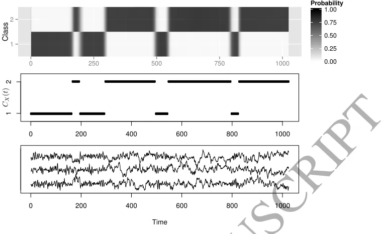
We simulate a set of 10 training signals using this model. The training signals each have the same class function which is initially in class 1 and then switches to class 2 half way through the time span. In order to test our method we simulate a group of 100 validation signals. The validation signals all have the same class function which is very different to the one used in the training set. This class function is initially in class 1 but switches 7 times at irregularly spaced intervals. We estimate the class membership probabilities for the validation signals using the method outlined in Section 3 and then take the mean.

ACCEPTED MANUSCRIPT

0 200 400 600 800 1000

Time 1

2

0 250 500 750 1000

Class

0.00 0.25 0.50 0.75 1.00

Probability

0 200 400 600 800 1000

1

2

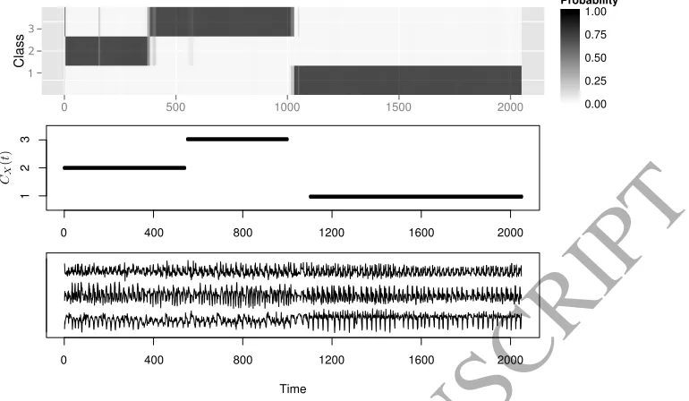
Figure 2: The upper plot shows the mean class membership probabilities for the 100 validation signals. The lower plot shows one of the validation signals. The middle plot shows the true class membership over time.

4.2

Example with Constant Auto-covariance

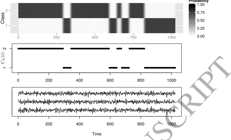
We now consider an example with a class specific cross-covariance structure and a constant auto-covariance structure. We again use an autoregressive process where, unlike the previous example, the AR coefficients are not class specific. The general form of the signals is therefore,

Xt = 0.8Xt−1−0.5Xt−2+ξt, ∀t∈ {0, T −1}. (10)

The set of random elements,_{ξ_t}again follow a normal distribution with zero mean and covariances defined in equation (9).

ACCEPTED MANUSCRIPT

0 200 400 600 800 1000

Time 1

2

0 250 500 750 1000

Class

0.00 0.25 0.50 0.75 1.00

Probability

0 200 400 600 800 1000

1

2

Figure 3: The upper plot shows the mean class membership probabilities for the group of 100 validation signals. The lower plot shows one of the validation signals. The middle plot shows the true class membership over time

as for the example in Section 4.1.

4.3

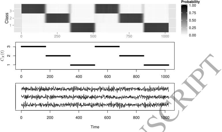
Example with Three Classes

Our final simulated example considers a scenario where Nc > 2. A third class is added to the example in Section 4.2. The AR coefficients will remain constant as in equation (10) however for time points where CX(t) = 3 the random elements {ξ_t} will be taken from a normal distribution with covariance matrix given by,

Σ(3)=

     

1 0.4 ₋0.6 0.4 1 0

−0.6 0 1

     

ACCEPTED MANUSCRIPT

0 200 400 600 800 1000

Time 1

0 250 500 750 1000

Class

3

2

0.00 0.25 0.50 0.75 1.00

Probability

0 200 400 600 800 1000

1

2

3

Figure 4: The upper plot shows the mean class membership probabilities for the group of 100 validation signals. The lower plot shows one of the validation signals. The middle plot shows the true class membership over time.

possible to see that there are slightly larger regions of uncertainty around the class transitions. This demonstrates that by adding a third class we have made the classification problem more challenging leading to greater uncertainty.

5

Accelerometer Data Example

ACCEPTED MANUSCRIPT

accelerometer was oriented the same way with respect to gravity and remained in place for the duration of the experiment. This ensured that the three channels could be directly compared between each repetition. Each recording is trimmed to be of length T = 2048. Since we do not expect the accelerometer to experience any changes in orientation, but rater oscillate around a fixed orientation, we expect the recorded signals to have a constant mean with any information relating to activity-type (walk, climb up stairs, climb down stairs) captured in the second order structure.

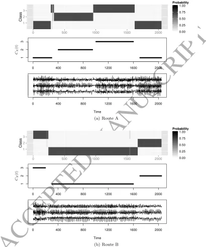
To illustrate our method we randomly select one repetition from each of Routes A and B, as well as the single repetition of Route C as our test set. The remaining 10 repetitions will be used as a training set. We adopt a three class model with class 1 being walking along the corridor, class 2 being walking up the stairs and class 3 being walking down the stairs. Figure 5 shows the classification results for the signals of Routes A and B. In both cases the true class is given a high probability for nearly all time points, the only exception to this being around the first transition in the Route A signal where the highest probability is placed on class 3 when the true class is either 1 or 2. The middle plots show the true class memberships, it is noticeable that there are very clear shifts in the probabilities which follow the true class memberships.

Figure 6 shows the results of our classification method performed on the Route C repetition. Since this repetition follows Route C the resulting signal is unlike any in the training data which all follow Route A or Route B. Looking at Figure 6 we see that our method is able to place a high probability on the true class for the majority of time points meaning that we can say what activities the participant is performing during Route C.

6

Discussion and Future Work

ACCEPTED MANUSCRIPT

Time 1

Class

3

2

0.00 0.25 0.50 0.75 1.00

Probability

1

2

3

400 800 1200 1600 2000

0

400 800 1200 1600 2000

0

500 1000 1500 2000

0

(a) Route A

Time 1

Class

3

2

0.00 0.25 0.50 0.75 1.00

Probability

1

2

3

400 800 1200 1600 2000

0

400 800 1200 1600 2000

0

500 1000 1500 2000

0

(b) Route B

ACCEPTED MANUSCRIPT

Time 1

Class

3

2

0.00 0.25 0.50 0.75 1.00

Probability

1

2

3

400 800 1200 1600 2000

0

400 800 1200 1600 2000

0

500 1000 1500 2000

0

Figure 6: Class probabilities for Route C. The upper plots show the estimated class probabili-ties. The lower plots show the accelerometer recordings. The middle plot shows the true class memberships.

ACCEPTED MANUSCRIPT

Acknowledgements

The authors are grateful to the anonymous reviewers for their constructive comments and sugges-tions that have significantly improved the quality of this manuscript. Park gratefully acknowledges funding from the EPSRC-funded STOR-i Centre for Doctoral Training and Unilever Research. Eck-ley’s work was supported by the Engineering and Physical Sciences Research Council under grant EP/I01697X/1, whilst Ombao gratefully acknowledges funding from NSF DMS and NSF SES.

References

[1] Ainsleigh, P. L., Kehtarnavaz, N., and Streit, R. L. Hidden Gauss-Markov models for signal classification. Signal Processing, IEEE Transactions on, 50, 6 (2002), 1355–1367. [2] B¨ohm, H., Ombao, H. C., von Sachs, R., and Sanes, J. Classification of multivariate

non-stationary signals: The SLEX-shrinkage approach. Journal of Statistical Planning and Inference 140, 12 (Dec. 2010), 3754–3763.

[3] Brillinger, D. Time series: data analysis and theory, vol. 36. SIAM, 2001.

[4] Caiado, J., Crato, N., and Pe˜na, D. A periodogram-based metric for time series classifi-cation. Computational Statistics & Data Analysis 50, 10 (June 2006), 2668–2684.

[5] Capp´e, O. A Bayesian approach for simultaneous segmentation and classification of count data. Signal Processing, IEEE Transactions on 50, 2 (2002), 400–410.

[6] Capp´e, O., Moulines, E., and Ryden, T. Inference in Hidden Markov Models. Springer Series in Statistics. Springer, 2006.

[7] Dahlhaus, R.Fitting time series models to nonstationary processes.The Annals of Statistics 25, 1 (1997), 1–37.

[8] Dahlhaus, R. Locally stationary processes. The Handbook of Statistics 30 (2012), 351–413. [9] Eckley, I., and Nason, G. Efficient computation of the discrete autocorrelation wavelet

ACCEPTED MANUSCRIPT

[10] Fisher, R. Frequency distribution of the values of the correlation coefficient in samples from an indefinitely large population. Biometrika 10, 4 (1915), 507–521.

[11] Fryzlewicz, P., and Ombao, H. C. Consistent classification of nonstationary time series using stochastic wavelet representations. Journal of the American Statistical Association 104, 485 (Mar. 2009), 299–312.

[12] Gianfelici, F.Rbf-based technique for statistical demodulation of pathological tremor.IEEE Transactions on Neural Networks and Learning Systems 24, 10 (Oct 2013), 1565–1574. [13] Gianfelici, F., and Farina, D. An effective classification framework for brain-computer

interfacing based on a combinatoric setting. IEEE Transactions on Signal Processing 60, 3 (March 2012), 1446–1459.

[14] Gott, A. N., and Eckley, I. A. A note on the effect of wavelet choice on the estimation of the evolutionary wavelet spectrum. Communications in statistics-simulation and computation 42 (2013), 393–406.

[15] Gott, A. N., Eckley, I. A., and Aston, J. A. D. Estimating the population local wavelet spectrum with application to non-stationary functional magnetic resonance imaging time series. Statistics in Medicine 34 (2015), 3901–3915.

[16] Huang, H.-Y., Ombao, H. C., and Stoffer, D. S. Discrimination and classification of nonstationary time series using the SLEX model. Journal of the American Statistical Associ-ation 99, 467 (Sept. 2004), 763–774.

[17] Huang, N. E., Shen, Z., Long, S. R., Wu, M. C., Shih, H. H., Zheng, Q., Yen, N.-C., Tung, C. C., and Liu, H. H. The empirical mode decomposition and the hilbert spectrum for nonlinear and non-stationary time series analysis. Proceedings of the Royal Society of London A: Mathematical, Physical and Engineering Sciences 454, 1971 (1998), 903–995. [18] Isserlis, L. On a formula for the product-moment coefficient of any order of a normal

ACCEPTED MANUSCRIPT

[19] Kakizawa, Y., Shumway, R. H., and Taniguchi, M. Discrimination and Clustering for Multivariate Time Series. Journal of the American Statistical Association 93, 441 (1998), 328–340.

[20] Krzemieniewska, K., Eckley, I., and Fearnhead, P. Classification of non-stationary time series. Stat 3, 1 (2014), 144–157.

[21] Krzemieniewska, K. I. Classification of non-stationary time series, 2013.

[22] Learned, R., Karl, W., and Willsky, A. Wavelet packet based transient signal classifi-cation. Time-Frequency and Time-Scale Analysis, 1992., Proceedings of the IEEE-SP Inter-national Symposium (1992), 109–112.

[23] Liu, S., and Maharaj, E. A. A hypothesis test using bias-adjusted AR estimators for classifying time series in small samples. Computational Statistics & Data Analysis 60 (Apr. 2013), 32–49.

[24] MacDonald, I., and Zucchini, W. Hidden Markov and Other Models for Discrete- valued Time Series. Chapman & Hall/CRC Monographs on Statistics & Applied Probability. Taylor & Francis, 1997.

[25] Meenakshi, A., and Rajian, C. On a product of positive semidefinite matrices. Linear algebra and its applications 295 (1999), 9–12.

[26] Nam, C. F. H., Aston, J. A. D., Eckley, I. A., and Killick, R. The Uncertainty of Storm Season Changes: Quantifying the Uncertainty of Autocovariance Changepoints. Tech-nometrics 52 (2015), 194–206.

[27] Nason, G., von Sachs, R., and Kroisandt, G.Wavelet processes and adaptive estimation of the evolutionary wavelet spectrum. Journal of the Royal Statistical Society. Series B 62, 2 (May 2000), 271–292.

[28] Olsen, G., and Brilliant, S. Signal processing and machine learning for real-time classifi-cation of ergonomic posture with unobtrusive on-body sensors; appliclassifi-cation in dental practice.

ACCEPTED MANUSCRIPT

[29] Ombao, H., von Sachs, R., and Guo, W. SLEX analysis of multivariate nonstationary time series. J. Amer. Statist. Assoc. 100, 470 (2005), 519–531.

[30] Ombao, H. C., Raz, J. A., Strawderman, R. L., and Von Sachs, R. A simple gen-eralised crossvalidation method of span selection for periodogram smoothing. Biometrika 88

(2001), 1186–1192.

[31] Park, T., Eckley, I., and Ombao, H. Estimating Time-Evolving Partial Coherence Be-tween Signals via Multivariate Locally Stationary Wavelet Processes. IEEE Transactions on Signal Processing 62, 20 (2014), 5240–5250.

[32] Priestley, M. B. Spectral Analysis and Time Series. Academic Press, London, 1983. [33] Sakiyama, K., and Taniguchi, M. Discriminant analysis for locally stationary processes.

Journal of Multivariate Analysis 90, 2 (Aug. 2004), 282–300.

[34] Sanderson, J., Fryzlewicz, P., and Jones, M. Estimating linear dependence between nonstationary time series using the locally stationary wavelet model. Biometrika 97, 2 (2010), 435–446.

[35] Santhanam, B., and Maragos, P. Multicomponent am-fm demodulation via periodicity-based algebraic separation and energy-periodicity-based demodulation. IEEE Transactions on Commu-nications 48, 3 (Mar 2000), 473–490.

[36] Shumway, R. Discriminant analysis for time series. In Classification Pattern Recognition and Reduction of Dimensionality, P. Krishnaiah and L. Kanal, Eds., vol. 2 of Handbook of Statistics. Elsevier, 1982, pp. 1 – 46.

ACCEPTED MANUSCRIPT

Appendix

Proof of Proposition 1

We begin by reminding the reader of a result established by [31] which is relevant to this proof, namely that the variance of the LWS estimate,Sb_jk(p,q), can be expressed as,

VarnSb_jk(p,q)o=O(M_T−1) +O(T−1).

HereMT is the smoothing bandwidth used to calculateSb(_jkp,q). For this estimate to be both

asymp-totically unbiased and consistent [31] make the assumptions thatMT → ∞andMT/T →0 in the

limit asT _{→ ∞}. Given this we can express MT in the formMT =O(Tα) for someα∈(0,1). The

variance ofSb_jk(p,q) can then be expressed as a single order term, varSb_jk(p,q)=_O(T−α_).

We now consider the asymptotics of our classification procedure. Letµ_bk be a vector of length

N which contains the elements of bζ_j,k;X which will be used to distinguish the different classes. For simplicity we will consider the two class problem however the results are easily generalised to the more general case. We define the divergence criterion to be,

∆(µ_bk) = 1 2

(µ_bk−µ₂)0Σ₂−1(µ_bk−µ₂)

−(µb_k−µ₁)0Σ₁−1(µb_k−µ₁) + log|Σ2|

|Σ1|

. (11)

This divergence criterion is simply the difference between log-likelihoods under the two classes. We also define the classification decision rule,

D(µb_k) =

    

1 (estimateC(k) = 1) if ∆(µb_k)>0 2 (estimateC(k) = 2) if ∆(µb_k)_≤0

.

Suppose that the true class membership, C(k), is equal to 1. Here we want to show that the probability of misclassification goes to 0 as T _{→ ∞}. That is we want to show, Pr(D(µ_bk) = 2_|C(k) = 1)_→0, or equivalently, Pr(∆(µ_bk)_≤0_|C(k) = 1)_→0.

ACCEPTED MANUSCRIPT

2|C(k) = 1) → 0 in the same limit. This results immediately follows if we can establish that as

T → ∞ then δT(µbk) P

→ K ≥ 0, which is satisfied by the following two conditions in the limit a

T → ∞: A1: E[δT(µbk)]→K whereK >0 and A2: var (δT(µbk))→0,

Expectation of

δ

(

µ

b

)

We first consider the expectation of δT(µbk), E[δT(µbk)] =−

1 2TαE

(µ_bk−µ₁)0Σ₁−1(µ_bk−µ₁) + 1

2TαE

(µ_bk−µ₂)0Σ₂−1(µ_bk−µ₂) + 1

2TαE

log|Σ2|

|Σ1|

.

We note that the first term follows a chi-squared distribution with N degrees of freedom, the expectation of which is equal toN. We now focus on the second term,

E(µb_k−µ₂)0Σ−12 (µbk−µ2)

=E{(µb_k−µ₁) + (µ₁−µ₂)}0Σ−1₂ {(µb_k−µ₁) + (µ₁−µ₂)}, =E(µbk−µ1)0Σ−12 (µbk−µ1)

+ 2E(µbk−µ1)0Σ−12 (µ1−µ2)

+E(µ1−µ2)0Σ−12 (µ1−µ2)

.

=Etr{(µb_k−µ₁)0Σ−12 (µbk−µ1)}

+ (µ₁−µ₂)0Σ−12 (µ1−µ2),

=Etr{Σ−12 (µbk−µ1)(µbk−µ1)0}

+ (µ₁−µ₂)0Σ−12 (µ1−µ2),

=tr{Σ−12 Σ1}+ (µ1−µ2)0Σ−12 (µ1−µ2). (12)

Therefore,

E[δT(µbk)] =

1 2Tα

−N+ tr_{Σ−₂1Σ1}

+(µ₁₋µ₂)0Σ₂−1(µ₁₋µ₂) + log|Σ2|

|Σ1|

.

Using the results of Proposition 5 from [31], the variance covariance matrices can be expressed as,

Σc =

ACCEPTED MANUSCRIPT

Here Ac andBc are constant symmetric positive definite matrices. The expectation can then be

written as,

E[δT(µb_k)] = 1 2Tα

−N+ tr{B1A2}

+Tα(µ₁−µ₂)0B₂−1(µ₁−µ₂) + log|A2|

|A1|

.

SinceB2is positive definite then we can say (µ₁−µ₂)0B₂−1(µ₁−µ₂) =C for some constantC >0. Also, sinceA1 andB2 are symmetric and positive definite, [25] showed thatA1B2will be positive definite and so we can say that tr{B1A2}=D for someD >0. Finally the term |A2|/|A1| must be positive as bothA1andA2 are positive definite. Without loss of generality we assume that this term is equal toG∈(0,∞). We can therefore express the expectation as,

E[δT(µbk)] =

1

2Tα{−N+CT

α_{+D+ logG},}

=C 2 +

D−N+ logG

2Tα .

Clearly asT _{→ ∞}thenE[δT(µbk)]→C/2 whereC/2 is a positive constant therefore conditionA1

is satisfied.

Variance of

δ

(

µ

b

)

We now consider the variance ofδT(µb_k), var (δT(µb_k)) = 1

4T2αvar (µbk−µ1)0Σ−11(µbk−µ1)

+ 1

4T2αvar (µbk−µ2)0Σ−21(µbk−µ2)

+ 1

2T2αcov (µbk−µ1)0Σ−11(µbk−µ1),

ACCEPTED MANUSCRIPT

The first term is simply the variance of a chi-squared random variable withN degrees of freedom so is equal to 2N. We therefore focus on the second and third terms. Looking at the second term,

var (µb_k−µ₂)0Σ₂−1(µb_k−µ₂)

=Eh(µb_k−µ₂)0Σ₂−1(µb_k−µ₂) 2i

−E(µb_k−µ₂)0Σ−₂1(µb_k−µ₂) 2.

The second term in the above equation, E(µ_bk−µ₂)0_Σ−1

2 (µbk−µ2) 2

, is simply the square of the term found in equation (12). We therefore focus on the first term,

Eh(µ_bk−µ₂)0_Σ−1

2 (µbk−µ2) 2i

. For simplicity we make the substitution µ∗_{= (µb}

k−µ2),

Ehµ∗ 0Σ−₂1µ∗ 2i=Eµ∗ 0Σ−₂1µ∗µ∗ 0Σ−₂1µ∗,

=E  X i X j

µ∗_i Σ−₂1_ijµ∗_jX

i0

X

j0

µ∗_i0 Σ−₂1_i0_j0µ∗j0

 , =X i X j X i0 X j0

Σ−₂1_ij Σ−₂1_i0_j0E

µ∗_iµ∗_jµ∗_i0µ∗_j0,

=X i X j X i0 X j0

Σ−₂1_ij Σ−₂1_i0_j0

Eµ∗_iµ∗_jEµ∗_i0µ∗_j0

+E[µ∗_iµ∗_i0]Eµ∗_jµ∗_j0+Eµ∗_iµ∗_j0Eµ∗_iµ∗_j0 .

In the final step above we have used Isserlis’ theorem, [18], to split the expression into three terms. We label these asD1, D2 and D3. We also note that E

h

ACCEPTED MANUSCRIPT

Looking at these terms individually we have,

D1=

X

iji0j0

Σ−12

ij Σ −1 2 i0j0E

µ∗iµ∗j

Eµ∗i0µ∗j0,

= X iji0j0

Σ−12

ij Σ −1 2 i0j0 n

(Σ1)_ij(Σ1)_i0j0

+ (µ1−µ2)i(µ1−µ2)j(Σ1)_i0j0 + (µ1−µ2)i0(µ₁−µ₂)j0(Σ1)ij

+(µ₁−µ₂)i(µ1−µ2)j(µ1−µ2)i0(µ1−µ2)j0},

=X ij

Σ−12

ij(Σ1)ij

X

i0j0

Σ−12

i0j0(Σ1)_i0j0 +X

ij

Σ−12

ij(µ1−µ2)i(µ1−µ2)j X

i0j0

Σ−12

i0j0(Σ1)_i0j0

+X i0j0

Σ−12

i0j0(µ1−µ2)i0(µ₁−µ₂)j0 X

ij

Σ−12

ij(Σ1)ij +X

ij

Σ−12

ij(µ1−µ2)i(µ1−µ2)j

×X

i0j0

Σ−12

i0j0(µ1−µ2)i0(µ1−µ2)j0,

=trΣ−12 Σ1 2

+ 2 trΣ−12 Σ1 (µ1−µ2)0Σ−12 (µ1−µ2)

+(µ₁−µ₂)0Σ−12 (µ1−µ2) 2

,

ACCEPTED MANUSCRIPT

Following a similar procedure forD2,

D2=

X

iji0_j0

Σ−₂1_ij Σ−₂1_i0_j0E[µ∗iµ∗i0]E

µ∗_jµ∗_j0

,

= X

iji0_j0

Σ−₂1_ij Σ−₂1_i0_j0

n

(Σ1)ii0(Σ1)jj0

+ (µ₁₋µ₂)i(µ1−µ2)i0(Σ₁)_jj0

+ (µ₁₋µ₂)j(µ1−µ2)j0(Σ₁)_ii0

+(µ₁−µ₂)i(µ1−µ2)j(µ1−µ2)i0(µ₁−µ₂)_j0 ,

=trΣ−₂1Σ1Σ−21Σ1

+ 2(µ₁₋µ₂)0Σ−₂1Σ1Σ−21(µ1−µ2)

+(µ₁−µ₂)0Σ₂−1(µ₁−µ₂) 2.

Similarly D3=D2. Putting together we obtain,

var (µ_bk−µ₂)0Σ−₂1(µ_bk−µ₂)= 2trΣ₂−1Σ1Σ−21Σ1

+ 4(µ₁−µ₂)0Σ−₂1Σ1Σ−₂1(µ1−µ2)

+ 2(µ₁₋µ₂)0Σ₂−1(µ₁₋µ₂).

We now consider the covariance term in equation (13),

cov (µbk−µ1)0Σ−11 (µbk−µ1),(µbk−µ2)0Σ−12 (µbk−µ2)

=E(µbk−µ1)0Σ−11 (µbk−µ1)(µbk−µ2)0Σ−12 (µbk−µ2)

−E(µb_k−µ₁)0Σ−11 (µbk−µ1)

E(µb_k−µ₂)0Σ−12 (µbk−µ2)

.

Looking at the first term,

E(µbk−µ1)0Σ−11(µbk−µ1)(µbk−µ2)0Σ2−1(µbk−µ2)

= X

iji0j0

(Σ−11)ij(Σ−21)i0j0

ACCEPTED MANUSCRIPT

We again split this up into three terms,C1, C2 andC3,

C1=

X

iji0_j0

(Σ−₁1)ij(Σ2−1)i0_j0E[(µb_k−µ₁)_i(µb_k−µ₁)_j]

×E(µ_bk−µ₂)i0(µb_k−µ₂)_j0,

= X

iji0_j0

(Σ−₁1)ij(Σ−21)i0_j0(Σ₁)_ij(Σ₁)_i0_j0

+(Σ1)ij(µ1−µ2)i0(µ₁−µ₂)_j0 ,

=NtrΣ1Σ−21 +N(µ1−µ2)0Σ−21(µ1−µ2).

Similarly forC2,

C2=

X

iji0_j0

(Σ−₁1)ij(Σ2−1)i0_j0E[(µb_k−µ₁)_i(µb_k−µ₂)_i0]

×E(µb_k−µ₁)j(µbk−µ2)j0,

=X

iji0_j0

(Σ−₁1)ij(Σ−21)i0_j0(Σ₁)_ii0(Σ₁)_jj0,

=trΣ1Σ−11Σ1Σ−21 = tr

Σ1Σ−21 .

It can also be shown that C2=C3 therefore,

ACCEPTED MANUSCRIPT

Therefore,

var (δT(µb_k)) = 1 2T2α

N+ trΣ−₂1Σ1Σ−21Σ1

+ 2(µ₁−µ₂)0Σ−₂1Σ1Σ−₂1(µ1−µ2)

+(µ₁₋µ₂)0Σ−₂1(µ₁₋µ₂)₋trΣ1Σ−21 ,

= 1

2T2α[N+ tr{B2A1B2A1}

+ 2Tα(µ₁−µ₂)0B2A1B2(µ₁−µ₂)

+Tα(µ1−µ2)0B2(µ1−µ2) + 4tr{B1A2}.

Using similar arguments as for the expectation we can say that tr{B2A1B2A1} = F > 0 and (µ₁−µ₂)0B2A1B2(µ₁−µ₂) =H >0 and so we can say,

var (δT(µb_k)) = 1

2T2α[N+F + 2T

α_H+Tα_{C+ 4D],}

=2H+C 2Tα +

N+F +D

2T2α .

Clearly asT → ∞then var (δT(µb_k))→0 and so condition A2is satisfied. Since both conditions are now satisfied we have established that Pr(δT(µb_k)≤0|C(k) = 1)→0 as T → ∞.

Proof of Proposition 2

We now consider the case of the distance between classes diverging, i.e. _|µ₁₋µ_{2| → ∞} for a fixed

T. Here we define_|µ₁₋µ_2|=qPN_i=1|(µ₁)i−(µ2)i|. To this end we define a different scaling of

the divergence criterion,

δµ(µbk) =

∆(µbk) |µ1−µ2|

2,

= 1 2|µ1−µ2|

2

+ (µbk−µ2)0Σ2−1(µbk−µ2) −(µbk−µ1)0Σ1−1(µbk−µ1) + log|

Σ2| |Σ1|

ACCEPTED MANUSCRIPT

Following a similar logic to the proof of Proposition 1 we aim to show that in the limit|µ₁−µ₂| → ∞ the probability of misclassification, Pr(D(µb_k) = 2|C(k) = 1) will tend to 0. This is equivalent to showing that Pr(δµ(µb_k)≤ 0|C(k) = 1)→0 in the same limit which immediately follows if we satisfy the following conditions in the limit as|µ₁−µ₂| → ∞: B1: Eδµ(µb_k)→K whereK >0 andB2: var δµ(µb_k)→0.

Expectation

We first consider the expected value ofδ_µ(µ_bk). Using the results from the proof of Proposition 1 it is readily seen that,

Eδµ(µ_bk)= 1 2_|µ₁₋µ_2|2

−N+ tr_{Σ−₂1Σ1}

+(µ₁₋µ₂)0Σ₂−1(µ₁₋µ₂) + log|Σ2|

|Σ1|

.

We assume that the terms N, tr{Σ−₂1Σ1} and log|Σ2|/|Σ1| do not depend upon the distance

between classes and so we will replace these three terms by the constant Q. We now consider the third term in the bracket, (µ₁−µ₂)0Σ−₂1(µ₁−µ₂). First we rewrite (µ₁−µ₂) in the form,

(µ₁−µ₂) =|µ₁−µ₂|v,

wherev= [v1, . . . , vN]0 a vector of constants. The third term can then be rewritten,

(µ₁₋µ₂)0Σ−₂1(µ₁₋µ₂) =_|µ₁₋µ_2|2v0Σ−₂1v

=|µ₁−µ₂|2R,

whereRis a positive constant due toΣ2, and thereforeΣ−21 being positive definite. Putting these

terms into the expectation we get,

Eδ_µ(µ_bk)= Q

2|µ₁−µ₂|2 +

R

2.

ACCEPTED MANUSCRIPT

Variance

We now consider the variance ofδ_µ(µ_bk). Using the results from Section 6 we can say that, var δµ(µb_k)= 1

2_|µ₁₋µ_2|4

N+ trΣ−₂1Σ1Σ−21Σ1

+ 2(µ₁₋µ₂)0Σ−₂1Σ1Σ−21(µ1−µ2)

+(µ₁−µ₂)0Σ−₂1(µ₁−µ₂) + 2trΣ1Σ−21 .

We first look at the terms which do not depend on _|µ₁₋µ_2| namely N, trΣ−₂1Σ1Σ−21Σ1 and

trΣ1Σ−21 . These terms can again be collected into one constant term, U. We have already stated

that the fourth term in the brackets can be written as_|µ₁₋µ_2|2R. The third term can also be re written,

2(µ₁₋µ₂)0Σ−₂1Σ1Σ−21(µ1−µ2)

=|µ₁−µ₂|2v0Σ−₂1Σ1Σ−21v

=_|µ₁₋µ_2|2V.

Putting these terms into the variance we get, var δµ(µb_k)= U

2|µ₁−µ₂|4 +

R+V

2|µ₁−µ₂|2.

Clearly in the limit |µ₁−µ₂| → ∞ then var δµ(µb_k) →0 and so the condition B2 is satisfied. We have therefore satisfied both conditions for this proof and have established that Pr(δµ(µb_k)≤

0_|C(k) = 1)_→0 as _|µ₁₋µ_{2| → ∞}.