FEA analysis and modelling of thermal stress in SOFCs
Dr Harald Schlegl (1), Dr Richard Dawson (1) (1) Lancaster University Engineering Dept.
Gillow Avenue, Lancaster LA1 4YW / United Kingdom
Tel.: +44 (0)1524 593685
[email protected], [email protected]
Abstract
Durability and reliability of anode supported SOFC stacks have proven unsatisfactory in large scale trials, showing rapid failure, thermal cycling intolerance and step change in electrochemical performance most likely related to mechanical issues. Monitoring and understanding the mechanical conditions in the stack especially during temperature changes can lead to improvements of the design and of the operating regime targeting maximum durability. Within this project modelling and simulation of thermal stresses within the different parts of the cells and the stack and the validation of this models play a key role and were performed in this work.
The modelling and simulation of stress and strain have been carried out using the FEA software ABAQUSTM. Model variations documented the importance of exact knowledge of material properties like Young’s modulus, Poisson’s ratio, thermal expansion coefficient, thermal conductivity and creep viscosity. The benefit of literature data for these properties is limited by the fact that all these properties are highly dependent on the composition of materials but also on details of the fabrication process like mixing, fabrication technique and sintering temperature and duration. The work presented here is an investigation into the modelling techniques which can be most efficiently applied to represent anode supported solid oxide fuel cells and demonstrates the temperature gradient and constraint on the stresses experienced in a typical design.
Comparing different meshing elements representing the cell parts thin shell elements (S4R) provided the most efficiently derived solution. Tensile stress is most significant in the cathode layers reaching 155 MPa at working conditions. The stress relieving effect of creep led to a reduction of stress by up to 20% after 1000 hours at 750°C, reducing the tensile stress in the cathode area to maximal 121 MPa. Constraint between bipolar plates increases the tensile stress, especially in the cathode layers leading to a peak value of 161 MPa.
1 Introduction
Finite element analysis (FEA) investigations of thermal stress in planar fuel cells including residual stress have been carried out by Anandakumar [1], who modelled functionally graded SOFCs, and by Laurencin [2] and Pitakthapanaphong [3] using multi-layered systems. Laurencin [2] compared degradation effects in anode supported and electrolyte supported cells. Johnson [4] used a 3D reconstruction method to model the infrastructure and determined an effective Young’s modulus and an effective thermal expansion coefficient based on this microstructure. Clague [5] used FEA modelling of a planar SOFC to predict the stress during the whole life-cycle including fabrication, anode reduction and operation under different loads. FEA analysis of thermal stress in SOFC cells of tubular and micro-tubular design has, amongst others, been carried out by Nakajo [6] and Cui [7]. The key requirement for realistic results of thermal stress calculated by FEA software is the input of reliable material data like Young’s Modulus, Poisson’s Ratio, Thermal Expansion Coefficient and creep coefficient for all materials involved in the model. Finding material data by experiments is time consuming, expensive and the results would need to be validated by comparing them to literature values to be reliable. Material data for common SOFC materials and composites like Ni/YSZ, YSZ, CGO, CGO/LSCF and LSCF, which are used in the cell studied in this work, are widely available from literature, however, the values depend on fabrication details of the tested materials. Parameters like particle size of the used powders, way of fabrication, sintering temperature and presence of pore formers influence the microstructure of the tested sample and the material properties.
Selcuk [8], Pihlatie [9] and Jia [10] agree in the opinion that the key factor for Young’s Modulus and Poisson’s Ratio of the composite Ni/YSZ anode is porosity rather than chemical composition, while the thermal expansion coefficient is increasing with increasing NiO and Ni content according to Mori [11] and Johnson [4]. Radovic [12] studied the thermal conductivity of the Ni/YSZ cermet and found values increasing from 4 W/mK to over 6 W/mK if the porosity is decreased from 40% to 26%. The elastic properties of the YSZ electrolyte depends on the percentage of yttrium oxide, sintering temperature and bulk density according to Giraud [13] and Adams [14] and additionally on the pO2 value of the atmosphere they were tested in according to Kushi [15]. The values for the
Young’s Modulus at room temperature differ from 165 GPa [12] to 220 GPa [14]. Biswas [16] found that the thermal expansion coefficient of YSZ decreases with increasing amount of yttria in YSZ. Additional to the factors important for YSZ, the percentage of cerium reduced from Ce4+ to Ce3+ plays a role for the values of both thermal expansion coefficient and Young’s Modulus as described by Hayashi [17] and Kushi [15]. CGO/LSCF composite materials differ in their elastic properties mainly due to different porosity according to a study by Chen [18] and in their thermal expansion coefficient due to different percentage of the components of the composite according to Li [19].
2 Simulation
model
2.1 Geometry
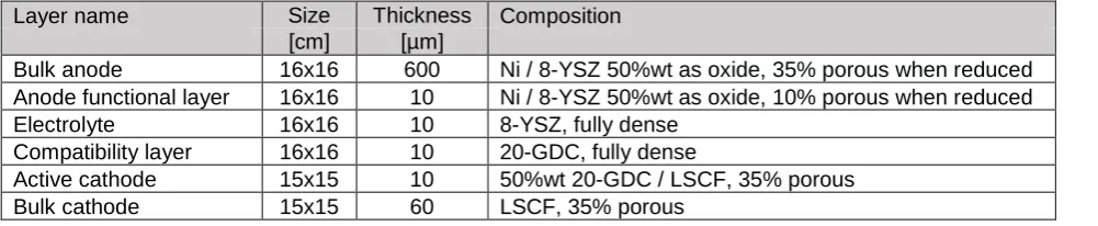
In this study a 16x16cm square planar cell was modelled in the way schematized in figure 1a. In the center of the cell is a 15x15cm active area with a thickness of 700 µm, comprised of two anode layers, an electrolyte layer, a compatibility buffer layer and two cathode layers. The inactive area at the border of the cell has a width of 0.5 cm and with a thickness of 630 µm it is slightly thinner because it lacks the two cathode layers. A summary of the chemical composition of each of the layers is displayed in table 1. Since the cell is symmetric along the x-axis, only half of the cell was modelled. The size and specification of the cell is typical of what could be considered for use within a stack with around 1-5 kW electrical output.
Figure 1: Schematic of the cell geometry of a) an unconstrained cell and b) a cell constrained between two bipolar plates. Dimensions are shown in mm.
Layer name Size Thickness Composition
[cm] [µm]
Bulk anode 16x16 600 Ni / 8-YSZ 50%wt as oxide, 35% porous when reduced Anode functional layer 16x16 10 Ni / 8-YSZ 50%wt as oxide, 10% porous when reduced Electrolyte 16x16 10 8-YSZ, fully dense
Compatibility layer 16x16 10 20-GDC, fully dense
Active cathode 15x15 10 50%wt 20-GDC / LSCF, 35% porous
[image:3.595.71.464.222.505.2]Bulk cathode 15x15 60 LSCF, 35% porous
[image:3.595.30.531.567.670.2]2.2 Materials
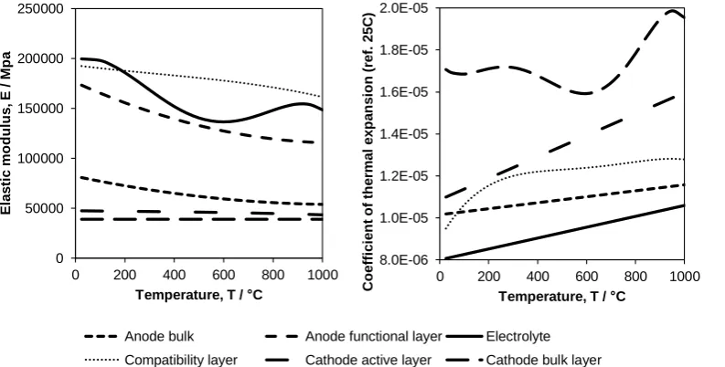
The physical materials properties of these layers where derived from the compiled data from Nakajo [20] as a self-consistent dataset. The important properties for the analysis are the elastic modulus, poissons ratio (though the variation in this value is less extreme), coefficient of thermal expansion and creep. This allows differences in thermal expansion coefficient to drive thermal stresses resisted by the layer stiffness’s. Creep is critical as a stress relief mechanism and is particularly important for the anode which has the least creep resistance of the layers. It therefore allows for some stress relief or change in stress field in the composite layers during operation.
Figure 1 summarises the temperature dependent modulus and expansion coefficient data used in the model. These data have been smoothed to allow more efficient solving in Abaqus whilst still retaining sufficient resolution for the analysis. The effect of porosity on the reduction of the elastic modulus is accounted for as described by Nakajo [20].
0 50000 100000 150000 200000 250000
0 200 400 600 800 1000
E
la
s
ti
c
m
o
d
u
lu
s
,
E
/
M
p
a
Temperature, T / C
Anode bulk Anode functional layer Electrolyte
Compatibility layer Cathode active layer Cathode bulk layer 8.0E-06
1.0E-05 1.2E-05 1.4E-05 1.6E-05 1.8E-05 2.0E-05
0 200 400 600 800 1000
C
o
e
ffi
c
ie
n
t
o
f
th
e
rm
a
l
e
x
p
a
n
s
io
n
(
re
f.
25C)
Temperature, T / C
Figure 2: Elastic modulus and coefficient of thermal expansion data used in Abaqus model. (Anode functional layers and bulk layers are taken to have the same thermal expansion coefficient)
The creep model used in the simulation is the hyperbolic sine model which efficiently captures the effect of temperature and stress on creep strain rate. However, in the simulation performed only steady-state creep is considered. The creep model used is given below in equation 1 with the parameters used for each layer in table 2 below.
𝜀̇𝑐𝑟 = 𝐴(sinh(𝐵𝜎))𝑛exp (−∆𝐻 𝑅𝑇)
Equation 1: formula for the creep strain, where: εcr is the creep strain rate, A and B are constants, σ is the stress, ΔH the activation energy, n is the stress order, R is the universal gas constant and T the absolute temperature.
Layer name A B n ΔH / kJ K-1 mol-1
Bulk anode 4.0 5 x 10⁻⁴ 1.7 115
Anode functional layer 4.0 5 x 10⁻⁴ 1.7 115
Electrolyte 1.8 x 10⁵ 1 x 10⁻³ 0.5 320
Compatibility layer 3.5 x 10⁴ 5 x 10⁻⁴ 1.0 264
Active cathode 3.5 x 10⁴ 5 x 10⁻⁴ 1.0 264
[image:4.595.104.501.247.448.2]Bulk cathode 6.0 x 10¹² 5 x 10⁻⁴ 1.7 392
[image:4.595.32.439.670.760.2]2.3 Simulation meshing elements
The cells themselves are often thin planar structures with dissimilar materials and in the case of some layers very differing thicknesses. This presents some difficulties in FEA as to how this can be most efficiently simulated since using traditional 3D continuum elements would require a very fine mesh. This means that stack simulations with many cells and the complexity of numerous multibody interactions would become very computationally intensive. In this study 4 different approaches were compared using the specialist element libraries available in AbaqusTM software. Four candidate representations that are considered to most accurately capture the stress and strain fields were considered in this work as a starting point for the simulation procedures to be used in the larger project. In each case the simulations considered temperature dependent creep, thermal expansion coefficient and elastic modulus. The mesh density was kept constant though the number of integration points (where stress and strain calculations are resolved) differs with the element type used.
(A) Thin shell element method (S4R elements). This uses 4 node elements but with 5 integration points per layer. These elements capture bending and membrane stresses efficiently but have only a 2D planar representation which can lead to some difficulties in defining interactions with other bodies.
(B) Continuum shell methods (SC6R elements). This is similar in definition to the thin shell element method only the elements have a 3D representation making interaction with other bodies simpler though the stiffness controls are less comprehensive.
(C) Incompatible modes methods (C3D8I elements). This is a hybrid method using incompatible modes 3D elements for the bulk anode with a ‘skin’ of the thinner layers (anode active – cathode bulk) in thin shell elements (S4R). Incompatible modes elements are good at capturing bending with only a single element through thickness of the beam. However, for the stress and bending result to be valid the C3D8I elements must be regular hexahedra limiting their application to square geometries.
(D) Standard continuum methods (C3D8R elements). This again is a hybrid method using the basic continuum element for the bulk anode with a ‘skin’ of S4R elements. The basic continuum element is fast to solve but requires a minimum of 4 elements through the thickness of the beam section to accurately capture bending.
To compare these representations a common set of simulation steps described in 3.5 were adopted for half symmetry models with a planar mesh density of 2.5 mm.
2.4 Boundary conditions and constraints
The unconstrained cell as depicted in figure 1a was bound at two points at the symmetric axis to prevent movement along the z-direction, referring to figure 1a these points have the coordinates (0/-80/0.63) and (0/80/0.63), one of these points additionally constrained the cell movement in the y-direction.
and to one point on each of the bipolar plates to prevent y-direction movement. (0/-80/2.63) and (0/80/-2)
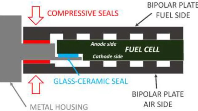
To provide an even more realistic perspective to the boundary conditions of the cell, the enclosure of this single cell and its bipolar plates inside a metal housing was added to the model. The sealing of the cells, the bipolar plates and the housing was simulated by a combination of compressive seals and glass-ceramic sealant as described in newer literature [22] and schematized in figure 3.
Figure 3: Schematic of the connection of a single cell with two interconnector plates and a metal housing using a combination of compressive seals and a glass-ceramic seal
2.5 Simulation steps and temperature distribution
Temperature fields were pre-defined and changed dependent on time and location to simulate the duty cycle of a planar element in a SOFC stack, starting with the simulation of a 1200 °C sintering period constituting the last production step of the cell.
At working conditions a temperature gradient along the y direction of the cell is caused by the exothermic oxidation of the fuel, occurring to a greater extent at the place the fuel enters the bipolar plate, so the fuel inlet side of each of the single cells is hotter than their fuel outlet side [23]. This temperature difference is increasing with increasing electrical load on the cell.
Experimental data about the temperature distribution in commercially available SOFC stacks is hardly ever published, the temperature distribution data available in literature is obtained from simulations or experimentally from lab designed and sized stacks. The difference in temperature between the cells located at different parts of the SOFC stack are reported to be less than 1 K [24] assuming highly thermal conductive metal cases, or in other cases up to 80 K [25], due to the temperature of the reaction gas being slightly lower than the average temperature of the stack.
[image:6.595.112.434.158.338.2]The simulation steps were as follows:
Cool from 1200 °C to an average operating temperature of either 720 °C, 750 °C, 780 °C or
800 °C with cells in a flat annealed state at the start. The simulated duration of this step was 10 hours
Apply a linear temperature distribution gradually over a simulated time of 30 minutes. This was to simulate progressive electrical loads on the cell. Five gradients were considered for each mean temperatures; no gradient, +/- 20 °C, +/- 40 °C, +/- 60 °C and +/- 80 °C.
Hold for 1,000 hours at operation temperature. This was to explore how creep of particularly the anode would affect the stress results.
This simulation procedure allowed the results between each method to be compared and the simulation time examined to determine which method can be most efficiently used to capture thermal stress and strains in a planar anode supported SOFC.
2.6 Basics of the mathematic algorithm
The driving force of the stress and strain changes with changing location and changing simulation conditions are the different thermal expansion coefficients of the geometry parts combined with changes of temperature. According to the thermo-mechanical model used by the FEA software, all parts undergo elastic deformation when subject to thermal load, the resulting thermal strain is calculated from equation 2.
Equation 2: formula for thermal strain in which εth is the thermal strain, α is the coefficient of thermal
expansion and Tref the stress-free temperature.
For isotropic solid materials with linear elastic behaviour the stress strain relationship follows equation 3.
Equation 3: formula for the stress strain relationship under thermal load, where E is the Young’s modulus, ν is the Poisson’s ratio, and σxx, σyy, σzz, σxy, σxz and σyz the normal stress and shear stress values in different
3 Results
3.1 Method comparison
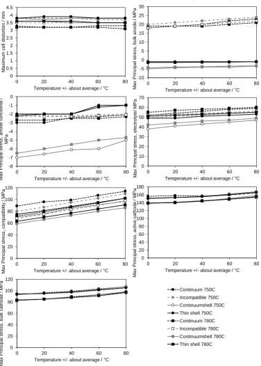
[image:8.595.108.485.162.689.2]The total cell distortion in the ‘z’ direction along with the peak principal stress values in the layers are displayed in Figure 4 at the start of the 1,000 hour hold and in Figure 5 at the end of the 1,000 hours. Each figure shows the effect of temperature gradient at the two operating temperatures and compares the 4 different modelling techniques. The model used for the comparison of different meshing elements is based on the unconstrained single cell as depicted in figure 1a.
Figure 4: Displacement and maximum principal stresses in layers at the start of the 1,000hour hold for
different operating temperature, temperature gradients and modelling techniques 0 0.5 1 1.5 2 2.5 3 3.5 4 4.5
0 20 40 60 80
M a xi m u m ce ll d ist o rt io n / m m
Temperature +/- about average / C
-10 -5 0 5 10 15 20 25 30
0 20 40 60 80
M a x P ri n ci p a l st re ss, b u lk a n o d e / M P a
Temperature +/- about average / C
-8 -7 -6 -5 -4 -3 -2 -1 0
0 20 40 60 80
M a x P ri n ci p a l st re ss, a n o d e f u n ct io n a l / M P a
Temperature +/- about average / C
0 10 20 30 40 50 60 70
0 20 40 60 80
M a x P ri n ci p a l st re ss, e le ct ro lyt e / M P a
Temperature +/- about average / C
0 20 40 60 80 100 120
0 20 40 60 80
M a x P ri n ci p a l st re ss, co m p a ti b ili ty / M P a
Temperature +/- about average / C
0 20 40 60 80 100 120 140 160 180
0 20 40 60 80
M a x P ri n ci p a l st re ss, a ct ive ca th o d e / M P a
Temperature +/- about average / C
0 20 40 60 80 100 120
0 20 40 60 80
M a x P ri n ci p a l st re ss, b u lk ca th o d e / M P a
Temperature +/- about average / C
Figure 5: Displacement and maximum principle stresses in layers at the end of the 1,000 hour hold for different operating temperature, temperature gradients and modelling techniques
With ceramic materials high tensile stresses can be considered to be potentially the most damaging since they have low fracture toughness, though buckling delaminations can occur if interfaces are weak and / or compressive load is extreme. These models assumed a well-developed interface not prone to delamination. Both Figures 3 and 4 show that both average operating temperature and thermal gradient are important when considering thermal stress. Figure 4 particularly shows that creep is important in stress relief but although the total strain energy is reduced in the model some layers can still be subjected to high stresses which may lead to damage and failure.
0 2 4 6 8 10 12 14
0 20 40 60 80
M a xi m u m ce ll d istr o ti o n / m m
Temperature +/- about average / C
-2 0 2 4 6 8 10 12 14
0 20 40 60 80
M a x P ri n ci p a l st re ss, b u lk a n o d e / M P a
Temperature +/- about average / C
-1 -0.5 0 0.5 1 1.5 2 2.5 3
0 20 40 60 80
M a x P ri n ci p a l st re ss, a n o d e f u n ct io n a l / M P a
Temperature +/- about average / C
0 5 10 15 20 25 30 35 40 45
0 20 40 60 80
M a x P ri n ci p a l st re ss, e le ct ro lyt e / M P a
Temperature +/- about average / C
0 20 40 60 80 100 120
0 20 40 60 80
M a x P ri n ci p a l st re ss, co m p a ti b ili ty / M P a
Temperature +/- about average / C
0 20 40 60 80 100 120 140 160
0 20 40 60 80
M a x P ri n ci p a l st re ss, a ct ive ca th o d e / M P a
Temperature +/- about average / C
0 10 20 30 40 50 60 70 80 90
0 20 40 60 80
M a x P ri n ci p a l st re ss, b u lk ca th o d e / M P a
Temperature +/- about average / C
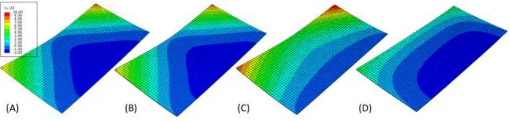
Predicting stress and strain variations in an unconstrained cell as in this simulation is (counter-intuitively), quite a difficult problem to simulate as slight differences in stiffness response allow initiation of different bending modes in notionally identical conditions. The displacements in these modes are then accentuated by creep during longer holds, such as that used here, which lead to a divergence in the predictions as can be seen in Figure 5. This is experienced in practice where cells in a furnace during manufacture will sometimes exhibit different final shapes due to slight differences in layers altering stiffness at a critical point in the process where the final distorted shape is influenced. Given this complexity the similarity in results before the 1,000 hour hold demonstrate that broadly either of the methods could be used though the standard continuum method can be seen to be the most different displaying high bulk anode stiffness and shape which is likely to unrealistic and caused by insufficient mesh density for this type of element. Examples of the final distorted shapes predicted for one of the simulations is shown in Figure 6. This shows clearly the difference between the two specialist shell element techniques and the incompatible modes and continuum techniques.
Figure 6: Final distorted shapes for 750°C operating temperature +/- 40 °C. (A) Thin Shell, (B) Continuum
shell, (C) Incompatible modes, (D) Standard continuum. Vertical displacements in mm, temperature increase to the right on each diagram. For the coloured version of the figures please see the online version of the paper.
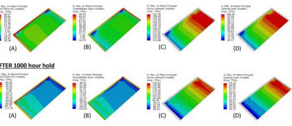
Figure 7: Stresses in selected layers for 750°C operating temperature +/- 40 °C. (A) electrolyte, (B) compatibility layer, (C) active cathode, (D) bulk cathode. Stresses are in MPa, temperature increase to the right on each diagram.
When considering the typical calculation time for each modelling as shown in Table 3 it is clear that using thin shell elements gives the most efficiently derived solution. An investigation into the sensitivity of the result to mesh density using thin shell elements shows that further understanding about the stress concentrations can be determined but in this case further geometric complexity such as radii at the corners of the cathode layers should be considered.
Method Shell Continuum shell Incompatible modes Continuum
Time / s 138 902 482 689
Table 3: Wall clock simulation times for different methods for 750°C operating temperature +/- 40 °C. Simulation was on intel CoreI7 using 2 CPUs and 16Gb RAM.
3.2 Constrained cell
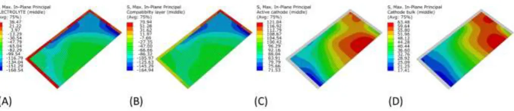
Figure 8: Stresses in selected layers for 750°C operating temperature +/- 40 °C. (A) electrolyte, (B) compatibility layer, (C) active cathode, (D) bulk cathode. Stresses are in MPa, temperature increase to the right on each diagram. Cell is constrained between ribbed bipolar plates with a load of 10 kg.
3.3 Cell constrained and sealed into a metal housing
The simulation assumes the metal housing and the pre-fabricated single cell to be assembled at room temperature. The residual stress in the different ceramic layers from the cool down step from 1200 °C adds to the stress caused by heating up the sealed stack to the working temperature of 750 °C +/- 40 °C. Since the metal housing has a slightly higher expansion coefficient than the ceramic layers of the cell, the connection with it during the heating step will cause additional tension to the ceramic layers. The results of the simulation of a cool down phase from 1200 °C to room temperature followed by heat up to working temperature and a 1000 hour hold period on the model of a cell sealed in the way described in section 2.4 and schematized in figure 3 are presented in figure 9. The comparison of the stress values of the sealed cell with the constrained cell stress values in figure 7 shows the expected decrease of compressive stress in the active area of the electrolyte (maximal -60 MPa instead of -115 MPa) and increase of tensile stress in the cathode area (maximal 161 MPa instead of 131 MPa). The average tensile stress in the inactive area of the electrolyte increased to around 50 MPa compared to around 20 MPa in figure 7, however locally there are peak values of 149 MPa tensile stress, in the compatibility layer even 189 MPa.
3.4 Influence of different cell temperature
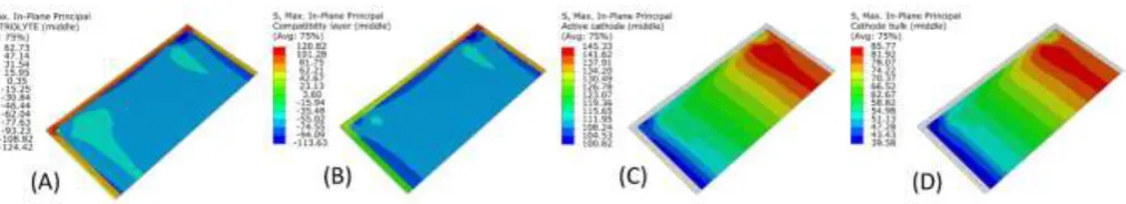
The stress and strain conditions in simulations of single cells with working temperatures of 720 °C +/- 40 °C, 750 °C +/- 40 °C and 800 °C +/- 40 °C were investigated to account for different cell temperatures at bottom, middle and top of a lab research long stack described in literature [25], the fuel gas in this particular literature case was fed at the bottom of the stack at a temperature of 625 °C. The simulation deals with a cell constrained between two bipolar plates using a load of 10 kg, same as in the simulation described in chapter 3.2. Using 1200 °C as a no-stress temperature, stress in all layers is supposed to be highest at the coldest location, the bottom cell with a working temperature of 720 °C +/- 40 °C, which was confirmed by simulation. Stress contours for the different cell layers are depicted in figure 10, they reveal a maximum tensile stress of 145 MPa in the active cathode layer, compared to 130 MPa at a working temperature of 750 °C +/- 40 °C (figure 8). The maximal compressive stress in the electrolyte layer is 124 MPa compared to the -115 MPa at a cell in the middle of the stack.
Figure 10: Stresses in selected layers for 720°C operating temperature +/- 40 °C. (A) electrolyte, (B) compatibility layer, (C) active cathode, (D) bulk cathode. Stresses are in MPa, temperature increase to the right on each diagram. Cell is constrained between ribbed bipolar plates with a load of 10 kg.
4 Validation
A solid oxide fuel single cell comparable to the simulated cell in composition and thickness of the layers was provided by HK Oil for experimental investigation. The cell was heated from room temperature to 800 °C in a lab furnace with quartz windows allowing optical access. The strain caused by the thermal expansion of the cell was measured by a 3D video gauging system and compared to the strain results of the simulation of a heat up from room temperature to 800 °C using the model of the unconstrained cell also used in the simulations described in chapter 3.1. The strain experimentally measured from the HK Oil cell in the lab furnace prove to be 5.15 % larger than the strain predicted by the FEA simulation, which is probably due to slight inaccuracies in material data and boundary conditions. The reasonably good accordance between the measured and computed strain values can, however, validate the stress and strain results from the simulations presented in this paper.
5 Conclusions
[image:13.595.50.556.241.333.2]Acknowledgements
The authors would like to thank the EPSRC for funding, their project partners for support and NVidia for the donation of a GPU for acceleration of solutions in larger modes. We like to thank our partners within the project “Novel diagnostic tools and techniques for monitoring and control of SOFC stacks – understanding mechanical and structural change” at Loughborough University and Imperial College, the POSTECH institute of new and renewable energy, Hankook Oil and the Korea Institute of Energy Research (KIER), particularly Dr. Jong-Won Lee.
The help of Dr. Ralph Clague with ABAQUSTM modelling and simulation and Mr. Peter Jones and Mr. Andrew Gavriluk with practical work and IT solutions is very much appreciated.
References
1 Anandakumar G, Li N, Verma A, Singh P, Kim J. Thermal stress and probability of failure analyses of functionally graded solid oxide fuel cells. Journal of Power Sources 2010; 195:6659-6670.
2 Laurencin J, Delette G, Lefebvre-Joud F, Dupeux M. A numerical tool to estimate SOFC mechanical degradation: Case of the planar cell configuration. Journal of the European
Ceramic Society 2008; 28:1857-1869.
3 Pitakthapanaphong S, Busso E. Finite element analysis of the fracture behavior of multi-layered systems used in solid oxide fuel cell applications. Modelling and Simulation in
Materials Science and Engineering 2005; 13:531-540.
4 Johnson J, Qu J. Effective modulus and coefficient of thermal expansion of Ni-YSZ porous cermets. Journal of Power Sources 2008; 181:85-92.
5 Clague R, Marquis A, Brandon N. Finite element and analytical stress analysis of a solid oxide fuel cell. Journal of Power Sources 2012; 210:224-232.
6 Nakajo A, Stiller C, Haerkegard G, Bolland O. Modelling of thermal stresses and probability of survival of tubular SOFC. Journal of Power Sources 2006; 158:287-294.
7 Cui D, Cheng M. Thermal stress modeling of anode supported micro-tubular solid oxide fuel cell. Journal of Power Sources 2009; 192:400-407.
8 Selcuk A, Atkinson A. Elastic properties of ceramic oxides used in solid oxide fuel cells.
Journal of the European Ceramic Society 1997; 17:1523-1532.
9 Pihlatie M, Kaiser A, Mogensen M. Mechanical properties of NiO/Ni-YSZ composites depending on temperature, porosity and redox cycling. Journal of the European Ceramic
Society 2009; 29:1657-1664.
10 Jia D, Zhou A, Ling Y, An K, Stoica A, Wang X. Effect of porosity on the mechanical properties of YSZ/NiO composite anode materials. World Journal of Engineering 2010; 7:489-495.
11 Mori M, Yamamoto T, Itoh H, Inaba H, Tagawa H. Thermal expansion of Nickel-Zirconia anodes in solid oxide fuel cells during fabrication and operation. Journal of the
Electrochemical Society 1998; 145:1374-1381.
12 Radovic M, Lara-Curzio E, Trejo R, Wang H, Porter W. Thermo-physical properties of Ni-YSZ as a function of temperature and porosity. Ceramic Engineering and Science Proceedings
2006; 27:79-85.
13 Giraud S, Canel J. Young’s modulus of some SOFC materials as a function of temperature.
Journal of the European Ceramic Society 2008; 28:77-83.
14 Adams J, Ruh R, Mazdiyashi K. Young’s modulus, flexural strength and fracture of yttria-stabilized zirconia versus temperature. Journal of the American Ceramic Society 1997; 80:903-908.
15 Kushi T, Sato K, Unemoto A, Hashimoto S, Amezawa K, Kawada T. Elastic modulus and internal friction of SOFC electrolytes at high temperatures under controlled atmospheres.
16 Biswas M, Kumbhar C, Gowtam D. Characterization of nanocrystalline YSZ: an in situ HTXRD study. International Scholarly Research Notices 2011;Article ID 305687.
17 Hayashi H, Kanoh M, Quan C, Inaba H, Wang S, Dokiya M, Tagawa H. Thermal expansion of Gd-doped ceria. Solid State Ionics 2000; 132:227-233.
18 Chen Z, Wang X, Giuliani F, Atkinson A. Microstructural characteristics and elastic modulus of porous solids. Acta Materialia 2015; 89:268-277.
19 Li N, Smirnova A, Verma A, Singh P, Kim J. Preparation and characterization of LSCF/GDC cathode for IT-solid oxide fuel cell. Advances in Solid Oxide Fuel Cells VI: Ceramic
Engineering and Science Proceedings 2010; 31:43-50.
20 Nakajo A, Kuebler J, Faes A, Vogt U, Schindler H, Chiang L, Modena S, Van Herle J, Hocker T. Compilation of mechanical properties for the structural analysis of solid oxide fuel cell stacks. Constitutive materials of anode-supported cells. Ceramics International 2012; 38:3907–3927.
21 Crofer 22 APU data sheet. Available online at: http://www.vdm-metals.com/
22 Smeacetto F, Salvo M, Santarelli M, Leone P, Ortigoza-Villalba G.A, Lanzini A, Ajitdoss L.C, Ferraris M. Performance of a Glass-Ceramic Sealant in a SOFC Short Stack. CInternational
Journal of Hydrogen Energy 2013; 38(1):588–596.
23 Liu Y, Cheng H, Hua J, Li X. Quantitative Analysis of Temperature Distribution in Cross-Flow Planar SOFC Based on a Validated Model. Conference paper Chinese Automation Congress
(CAC) Wuhan 2015; 1192–1196.
24 Nikooyeh K, Ayodeji A.J, Hill J.M. 3D Modeling of Anode-Supported Planar SOFC with Internal Reforming of Methane. Journal of Power Sources 2012; 171(2):601–609.