warwick.ac.uk/lib-publications
A Thesis Submitted for the Degree of PhD at the University of Warwick
Permanent WRAP URL:
http://wrap.warwick.ac.uk/105768
Copyright and reuse:
This thesis is made available online and is protected by original copyright. Please scroll down to view the document itself.
Please refer to the repository record for this item for information to help you to cite it. Our policy information is available from the repository home page.
Supervisors:Dr. Nikola P. Chmel, Prof. Alison Rodger, Dr. Vasily Kantsler and Prof. Ravi Jagadeeshan
A thesis submitted in partial fulfilment of the requirements for the degree of
Doctor of Philosophy
Molecular Organisation and Assembly in Cells (MOAC)
Doctoral Training Centre, University of Warwick
Contents i
List of Tables vi
List of Figures ix
List of Abbreviations xx
Acknowledgements xxiii
Declaration xxv
Abstract xxvi
1 Introduction 1
1.1 Absorbance and linear dichroism . . . 2
1.2 LD experiments with polymers in solution . . . 9
1.3 Simulating polymers in dilute solutions . . . 10
1.4 Studying the structure of membrane proteins . . . 16
1.5 Aligning vesicles in fluid flow . . . 21
1.6 Microfluidic experiments with vesicles . . . 28
1.7 Thesis outline . . . 32
2 Using FENE-Fraenkel springs in polymer simulations 33 2.1 Spring Force Law Formulation . . . 34
2.1.1 FENE springs . . . 34
2.1.2 Fraenkel springs . . . 35
2.3.2 Obtaining the Fraenkel law from FENE-Fr. law . . . 41
2.4 Zero-shear rate equilibrium properties . . . 42
2.4.1 Calculating equilibrium properties . . . 42
2.4.2 Potential functionφfor a dumbbell . . . 44
2.4.3 Equilibrium properties of the length of a FENE-Fraenkel spring . 45 2.5 Excluded Volume Force Law . . . 54
2.6 Hydrodynamic interactions . . . 55
2.7 Numerical method for solving the bead-spring configuration . . . 56
2.7.1 Bead-Spring Configuration Equation . . . 56
2.7.2 Discretisation — Step 1 — First guess . . . 59
2.7.3 Discretisation — Step 2 — Updated guess . . . 60
2.7.4 Discretisation — Step 3 — Recasting the updated guess . . . 60
2.7.5 Discretisation — Step 4 — Generating a cubic . . . 62
2.8 Summary . . . 63
3 Simulating polymers in flow with FENE-Fraenkel springs 64 3.1 Code alterations to incorporate the FENE-Fraenkel spring . . . 64
3.2 Verification of simulation against analytically derived properties . . . 66
3.2.1 Zero-shear conditions . . . 66
3.2.2 Non-zero shear conditions . . . 69
3.3 Comparison against work by Hsieh et al. [48] . . . 72
3.3.1 Conversion between parameter values . . . 72
3.3.2 Choice ofH∗and its influence on simulated polymer stresses . . . 75
3.3.3 Choice ofδ∗and its influence on simulated polymer stresses . . . 79
3.3.4 Choice of∆t∗and its influence on simulated polymer stresses . . 83
3.4 Orientation behaviour of a FENE-Fraenkel dumbbell in linear shear flows
with and without hydrodynamic interactions . . . 89
3.5 Summary and future work . . . 100
4 Development of planar microfluidic devices for linear dichroism studies 102 4.1 LD experiments using Couette Flow . . . 103
4.2 Absorbance of PDMS . . . 104
4.3 Preparation of planar microfluidic channels . . . 106
4.3.1 Making the silicon wafer cast . . . 106
4.3.2 Manufacture of the PDMS microfluidic channel from the cast . . 110
4.4 Preliminary experiments with microfluidic devices . . . 111
4.4.1 Results with wide channel . . . 113
4.4.2 Results with zig-zag channel . . . 116
4.4.3 Analysis of results . . . 119
4.5 Development of an extensional flow device . . . 120
4.6 Measuring and modifying the path length of microfluidic devices . . . 124
4.6.1 Using light inteferometry to measure channel depth of devices . . 124
4.6.2 Increasing path length and measuring channel depths using light interferometry . . . 126
4.6.3 Using potassium chromate absorbance to measure channel depth . 128 4.7 Experimental results with deeper microfludic devices . . . 130
4.7.1 Couette shear flow . . . 130
4.7.2 Poiseuille (pressure-driven) flow in the deep wide channel . . . . 132
4.7.3 Extensional flow in the deep cross-slot . . . 134
4.7.4 Comparison of orientation performance . . . 136
4.8 Summary and future work . . . 138
5 Linear dichroism experiments with vesicles in flow 139 5.1 Introduction — Lipids, vesicles and DPH . . . 140
5.2 Initial protocol for vesicle preparation . . . 143
5.3 Experiments with Couette flow and the wide channel microfluidic device . 146 5.4 Experiments with a shallow cross-slot microfluidic device . . . 149
5.7 Summary and future work . . . 168
6 Conclusions and future work 169 6.1 Implementation of the FENE-Fraenkel force law into bead-spring chain simulations . . . 169
6.2 Development of an extensional flow microfluidic device for use in LD experiments . . . 171
Bibliography 174 A Derivation of Equation (2.4.11) 190 B Fortran code documentation 193 B.1 sensemble.f90 . . . 193
B.2 modules.f90 . . . 196
B.3 utils.f90 . . . 196
B.4 gsipc.f90 . . . 198
B.5 properties.f90 . . . 201
C Alterations to the code to incorporate the FENE-Fraenkel spring 203 C.1 sensemble.f90 . . . 204
C.2 modules.f90 . . . 205
C.3 utils.f90 . . . 207
C.4 gsipc.f90 . . . 212
C.5 properties.f90 . . . 227
D Fortran code for simulations 228 D.1 sensemble.f90 . . . 228
D.3 utils.f90 . . . 252
D.4 gsipc.f90 . . . 270
D.5 properties.f90 . . . 299
E Vesicle preparation and method development 305 E.1 Vesicle size during manufacture . . . 305
E.1.1 Slow cycles . . . 307
E.1.2 Fast cycles . . . 309
E.2 Using purified lipids . . . 310
E.2.1 Using DOPC . . . 310
E.2.2 Using POPC . . . 312
F Supplementary figures from experiments with vesicles in Chapter 5 314 F.1 Additional figures referenced in Section 5.3 . . . 314
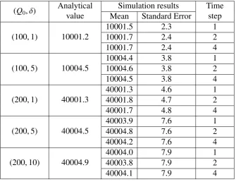
3.3 Mean values and standard errors forhR2iunder different linear shear rates and using a time step of 1 time unit. These have been averaged over the timepoints of the last 2000 time units of the 10000 time unit length simulation. . . 70 3.4 Values of various parameters under the non-dimensionalisation paradigm
of this work converted from the parameters used in [48] to analyse the effect of the choice of spring constant parameter on simulation results. . . 76 3.5 Averaged values for the mean and standard error of σ11 between
time-points 1.8 and 2.0 (the “plateau”) in simulations using parameters de-scribed in Table 3.4 and in [48, Figure 3]. . . 78 3.6 Values of various parameters under the non-dimensionalisation paradigm
of this work converted from the parameters used in [48] to analyse the effect of the choice of spring extensibility parameter on simulation results. 80 3.7 Averaged values for the mean and standard error of σ11 between
time-points 2.4 and 2.5 (the “plateau”) in simulations using parameters de-scribed in Table 3.6 and in [48, Figure 4]. . . 80 3.8 Values of various parameters under the non-dimensionalisation paradigm
3.9 Values of∆t∗tested to ascertain the effect of time-step size on our simula-tions, with values of the average mean and standard error forσ11between 1.97 and 2.03 time units (as scaled according to the simulation results of Hsieh et al. [48]). . . 86 3.10 Parameters used for simulations to assess the alignment of FENE-Fraenkel
dumbbells in shear flow. . . 89 3.11 Mean values and standard errors for the orientation parameter S (to 3
decimal places) under different linear shear rates, different time-step sizes and with or without hydrodynamic interactions present. These have been averaged over the timepoints of the last 20000 time units of the 100000 time unit length simulation. . . 94 4.1 Relationship between duration of soft bake stages and the thickness of the
SU-8 2100 photoresist layer desired. This table is reproduced with data from Table 2 of the Processing Guidelines for SU-8 2100 and SU-8 2150 photoresists by Microchem. . . 108 4.2 Relationship between UV light exposure energy doses and the thickness
of the SU-8 2100 photoresist layer desired. This table is reproduced with data from Table 3 of the Processing Guidelines for SU-8 2100 and SU-8 2150 photoresists by Microchem. . . 108 4.3 Relationship between duration of post exposure bake stages and the
thick-ness of the SU-8 2100 photoresist layer desired. This table is reproduced with data from Table 5 of the Processing Guidelines for SU-8 2100 and SU-8 2150 photoresists by Microchem. . . 109 5.1 Minimum flow rates required for flow in the cross-slot design to
over-come Brownian rotational forces, on the assumption of treating vesicles as spheres. . . 151 5.2 Mean vesicle diameters and associated standard deviations, based upon
DLS intensity measurements of 15 samples after each slow freeze-thaw cycle. . . 309 E.4 Mean vesicle diameters and associated standard deviations, based upon
1.1 An illustration of unpolarised and polarised light. A polariser is used to allow light of a particular polarisation to pass through (in this case, vertically polarised light); all other polarisations are blocked. . . 4 1.2 Dimensions of the Couette flow cell used for LD experiments. . . 7 1.3 Schematic of a Couette flow cell for LD experiments. . . 7 1.4 Example of a bead-spring chain with seven beads. In the Rouse model,
these springs are Hookean (the tension force is proportional to their length) and freely-jointed to the beads (meaning that there is no restriction on the angle between two springs attached to the same bead). . . 11 1.5 Graphs of cot 2χ and−∆A45/AagainstG, where χ is the angle between
the electronic transition of interest and the flow direction (corresponding toαin Equation (1.1.4)),Ais the isotropic absorbance,∆A45is the change in absorbance observed between the flow direction and 45° to the flow di-rection andG is the shear rate. These experimental data were obtained by studying DNA in flow. The lines plotted are using linear least-squres regression. Theory from Rouse-Zimm models suggests a linear relation-ship betweenGand observable variables cotχand−∆A45/A. This linear relationship is seen for low shear rates, but degenerates for values of G above 20 s−1. These figures are reproduced from Figures 1 and 2 of [164]. 14 1.6 Diagram defining the axes referred to in the expression for the orientation
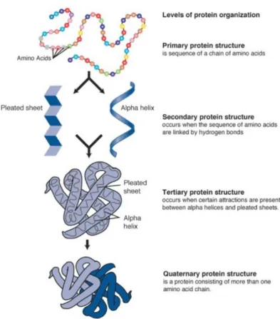
parameterS (Equation (1.3.4)). . . 15 1.7 Illustration of the basic components of phospholipids and a schematic
-helices -sheets
bonding; these make up the protein’s secondary structure. Further fold-ing and arrangements of the secondary structure gives rise to thetertiary structure. The collection of tertiary structures that make up a protein are known as thequartenary structure. A more detailed treatment of protein structure can be found in [75]. . . 18 1.9 Vesicle types based on diameter and lamellarity. This diagram is
repro-duced with permission from the Figure 2 of [55]. . . 21 1.10 An illustration of the three types of behaviour that vesicles undergo in
planar fluid-flow. The three lines corresponds with (from top to bottom) tank-treading (TT), trembling (TR) and tumbling (TB). These diagrams are reproduced with permission from the abstract figure of [2]. . . 22 1.11 A diagram illustrating the rotational (left) and extensional/elongational
(right) components of a linear shear flow (middle). Reproduced from Figure 2 of [2]. . . 24 1.12 Phase diagram illustrating the regions of (S,Λ)-parameter space that
cor-respond to the different vesicle behaviours. Tank-treading takes place in the blue and green regions, trembling in the area between solid red and broken blue lines and tumbling in the orange and grey areas. The diagram is reproduced from Figure 9 of [71]. . . 25 1.13 The elongation of a vesicle containing chromophores of interest in its
1.14 An illustration of the tilt of a vesicle away from a stationary boundary wall while in fluid shear flow. The vesicle is experiencing a lift force Fli f t, whose magnitude is dependent upon the shear rate ˙γ. This diagram is reproduced with permission from the abstract figure of [2]. . . 27 1.15 This diagram illustrates the cross-slot device used by Tanyeri et al. [147].
(a) A hydrodynamic trap is created by a planar extensional flow field at the junction of two perpendicular microchannels. (b) The velocity field (top) and the potential well (bottom) for a particle in the flow field at the microchannel junction. This diagram is reproduced with permission from Figure 1 of [147]. . . 29 1.16 The four-roll mill device used by Taylor [150]. Four rotating mills
con-trolled by driving pulleys cause the fluid drop in the centre to change shape. This diagram is reproduced with permission from Figure 1 of [150]. 30 1.17 (a) A macroscale summary of the roll mill. (b) The microfluidic
four-roll mill device used by Lee et al. [72]. All flow types can be generated by varying the angular velocity ratioω1/ω2or flow rate ratioQ1/Q2. These diagrams are reproduced with permission from Figure 1 of [72]. . . 30 2.1 An illustration of a spring vector of a spring in a bead-spring chain. . . . 34 2.2 An illustration of the relationship between the length and the spring
ten-sion of a FENE spring. The spring length can vary between zero inclusive and Qmax exclusive. The tension force increases in magnitude signifi-cantly as the spring length gets close to Qmax. . . 35 2.3 An illustration of the relationship between the length and the spring
ten-sion of a Fraenkel spring. The spring tenten-sion/compression force is lin-early proportional to the extension/compression from the natural spring lengthQ0. . . 36 2.4 An illustration of the relationship between the length and the spring
ff
derived value under zero shear conditions, using a FENE-Fraenkel spring with natural length Q0 = 200 and extensibility δ = 10. Standard error bars have been ommitted for clarity. Means and standard errors for the last 2000 time units of each simulation are given in Table 3.3. . . 71 3.3 Plots of σ11 against time for a 11-bead, bead-spring chain with
FENE-Fr springs under a uniaxial extensional flow, corresponding to different parameter combinations described in Table 3.4. Time scales of the simu-lations have been rescaled to match that of the data given in Hsieh et al. [48], each corresponding to a different value of spring constant (spring stiffness). The “Hsieh data” plot corresponds to data obtained from Fig-ure 3 in Hsieh et al. [48] . . . 77 3.4 Histogram of the deviations from the average value of σ11 along the
plateau of plots in Figure 3.3. . . 79 3.5 Plots ofσ11against time for a 11-bead, bead-spring chain with FENE-Fr
springs under a uniaxial extensional flow with different spring extensibil-ity values, as given in Table 3.6. Time scales of the simulations have been rescaled to match that of the data given in Hsieh et al. [48]. The “Hsieh data” plot corresponds to data obtained from Figure 4 in Hsieh et al. [48] . 81 3.6 Histogram of the deviations from the average value of σ11 along the
plateau of plots in Figure 3.5. . . 81 3.7 Magnification of the plots of Figure 3.5 in the plateau region between
3.8 Plots ofσ11against time for a 11-bead, bead-spring chain with FENE-Fr springs under a uniaxial extensional flow, corresponding to different time-step sizes, as described in Table 3.8. The “Hsieh data” plot corresponds to data obtained from [48, Figure 7]. Time scales of the simulations have been rescaled to match that of the data given in [48]. . . 84 3.9 Magnification of the plots of Figure 3.5 in the plateau region between
1.97 and 2.03 time units, including standard error bars at each time point (i.e. Equation (3.2.1) is applied but with data with respect to a single time point), for our simulations based on a sample size of 1000 independent trajectories. Hsieh data obtained from [48, Figure 7 Inset] using Plot Digitizer. . . 84 3.10 Plots of theσ11against time for a 11-bead, bead-spring chain with
FENE-Fr springs under a uniaxial extensional flow, restricted to the plateau re-gion between 1.97 and 2.03 time units (as scaled according to the simula-tion results of Hsieh et al. [48]) for a range of values of∆t∗as detailled in Table 3.9. The simulations were based on a sample size of 1000 indepen-dent trajectories. . . 86 3.11 Plots of theσ11against time for a 11-bead, bead-spring chain with
FENE-Fr springs under a uniaxial extensional flow, as in Figure 3.10, for a se-lection of values of ∆t∗. Standard error bars at a selection of time points are included (Equation (3.2.1) is applied but with data with respect to a single time point). . . 87 3.12 Plots of the orientation parameter S against time for different time-step
values and different linear shear rates ˙g without hydrodynamic interac-tions, using a FENE-Fraenkel spring with natural length Q0 = 100 and extensibilityδ= 1. Standard error bars have been ommitted for clarity. . . 95 3.13 Plots of the orientation parameter S against time for different time-step
teractions, using a FENE-Fraenkel spring with natural length Q0 = 100, extensibility δ = 1 and time-step size∆t = 0.5. Standard error bars have been ommitted for clarity. . . 98 3.16 Plots of the orientation parameter, S, against time for different particle
sizes and shear rates at 22°, as calculated from the model developed by McLachlan et al. [89]. aandbare the particle semi-diameters measured parallel and perpendicular, respectively, to the axis of revolution,kis the shear rate andλis the particle material time constant (see [14]). Subfigure (a) concerns shorter particles (b = 4 nm) or low shear rates. Subfigure (b) focusses on high shear rates for M13 bacteriophage particles (λ = 4.37 ms). The graphs are reproduced from Figure 2 of [89]. . . 99 4.1 Schematic of the Couette flow cell used for LD experiments. . . 103 4.2 Schematic of a Couette flow cell for LD experiments. . . 104 4.3 Absorbance spectra of polydimethylsiloxane (PDMS) samples with
dif-ferent thicknesses. . . 105 4.4 Relationship between final wafer rotation speed and the thickness of the
4.5 A photo of a Karl Suss MJB3 Mask Aligner, used for the exposure of silcon wafers with a photoresist layer to UV light. The mask is placed, photoresist layer on top, on the silver circular holder on the red plate. This is then moved into place under a glass in the exposure zone (located underneath the microscope). A vacuum holds the silicon wafer in place. The X-ray film with the design printed as a negative is placed on the glass just underneath the microscope — the “shiny” film side should be placed facing up. . . 109 4.6 An example of a finished silicon wafer cast with channel designs in
pho-toresist in the centre. Scotch®tape is attached to the wafer to form a well for the liquid PDMS to set. . . 110 4.7 “Wide Channel” . . . 111 4.8 “Zig-zag channel” . . . 111 4.9 Illustration of the use of an IR spectroscopy cell holder for the flow cell. . 112 4.10 Linear dichroism spectra of DNA solution passed through the wide
chan-nel microfluidic device at different flow rates. . . 113 4.11 Absorbance of DNA solution passed through the wide channel
microflu-idic device. . . 114 4.12 Reduced linear dichroism spectra of DNA solution passed through the
wide channel microfluidic device at different flow rates. . . 114 4.13 Estimated values of the orientation parameter (calculated using the
re-duced LD signal measured at 260 nm) against flow rate using the wide channel microfluidic device. . . 115 4.14 Linear dichroism spectra of DNA solution passed through the zig-zag
channel microfluidic device at different flow rates. . . 116 4.15 Absorbance of DNA solution passed through the zig-zag channel
mi-crofluidic device. . . 117 4.16 Reduced linear dichroism spectra of DNA solution passed through the
zig-zag channel microfluidic device at different flow rates. . . 117 4.17 Estimated values of the orientation parameter (calculated using the
central intersection, with arrows indicating the flow directions. . . 121 4.20 Details of particular lengths and radii of curvature for the Haward
cross-slot design used in the experiments reported in this thesis. . . 122 4.21 Surface profiler depth map of the orignal wide channel used for
prelimi-nary tests. . . 125 4.22 Dimensions of the revised wide channel design. . . 126 4.23 Surface profiler depth map of the deeper wide channel design on the
sil-icon wafer, as used for later experiments. The tilt that can be observed here is due to the configuration of the platform on which the wafer was placed, so as to allow the inteferometer to capture the light interference waveforms precisely. . . 127 4.24 Surface profiler depth map of the deeper cross-slot used for final tests. . . 127 4.25 Absorbance spectrum of 2 mM potassium chromate solution passes through
the cross-slot device. . . 129 4.26 Absorbance spectra of 2 mM potassium chromate solution through the
wide channel microfluidic device as it is pumped at different flow rates. . 129 4.27 Derived path length of the wide channel microfluidic device at different
flow rates. . . 130 4.28 Linear dichroism, absorbance and reduced LD spectra of DNA solution in
Couette flow at different rotation speeds. The measurements were taken with DNA solution prepared for use in the deep cross-slot microfluidic device. The results for the solution prepared for use in the deep wide channel device gave similar value for the reduced LD. . . 131 4.29 Linear dichroism & reduced LD spectra of DNA solution in
4.30 Linear dichroism, absorbance and reduced LD spectra of DNA solution in extensional flow through the deep cross-slot microfluidic device. . . 135 4.31 Linear dichroism & reduced LD spectra of DNA solution in extensional
flow through the deep wide channel microfluidic device and a plot of re-duced LD at 260 nm against flow rate. . . 137 5.1 Illustration of the basic components of phospholipids and a cross-section
of a phospholipid bilayer. . . 140 5.2 Distribution of fatty acids present in soy bean PC sourced from Sigma
Aldrich®P3644. The numerical X:Y labels refer to the number of carbons in the fatty acid chain (X) and the number of unsaturated carbon double bonds present in the chain (Y). . . 141 5.3 Absorbance spectrum of 1,6-diphenylhexa-1,3,5-triene (DPH) in methanol
(0.02 mg ml−1), with a diagram of a DPH molecule and an inset of the peaks between 250 nm and 280 nm. Peaks corresponding to long- and short-axis transitions are marked on the plot. . . 142 5.4 Diagram and photos of the Avanti Polar Lipids Mini-Extruder Kit used to
extrude lipid vesicle solutions. . . 145 5.5 Absorbance and LD spectra of soy bean PC vesicles containing DPH (0%,
2%, 4% and 10% by mass) in Couette shear flow and pressure-driven flow through the wide channel microfluidic device. The LD spectra of soy bean PC vesicles with 4% and 10% DPH by mass in pressure-driven flow are in the Appendices in Figure F.1 . . . 146 5.6 Vesicle size distribution data obtained using DLS for soy bean PC vesicles
containing 0% and 2% DPH by mass before use in flow experiments. . . . 148 5.7 Structures of three PC lipids with chains typical to those found in soy
bean PC. . . 152 5.8 Absorbance and LD spectra of soy bean PC vesicles without DPH and
5.11 Vesicle size distribution data (based on intensity measurements) obtained using DLS for soy bean PC vesicles with 0.4% DPH by mass, before and after use in the deep wide channel microfluidic device. . . 161 5.12 Linear dichroism and absorbance spectra of soy bean PC vesicles with
0.4% DPH by mass, in extensional flow through the deep cross-slot mi-crofluidic device at different flow rates. . . 163 5.13 Linear dichroism and absorbance spectra from Couette flow for soy bean
PC vesicles with 0.4% DPH by mass, before and after use in the deep cross-slot microfluidic device. . . 164 5.14 Vesicle size distribution data (based on intensity measurements) obtained
using DLS for soy bean PC vesicles with 0.4% DPH by mass, before and after use in the deep cross-slot microfluidic device. . . 165 E.1 Vesicle diameter distribution data (measured using intensity measurements
obtained with DLS) for soy bean PC vesicles after individual stages of the manufacture protocol. . . 306 E.2 Vesicle diameter distribution data (measured using intensity measurements
obtained with DLS) for soy bean PC vesicles after individual stages of the manufacture protocol. . . 308 E.3 Vesicle diameter distribution data (measured using intensity measurements
obtained with DLS) for soy bean PC vesicles after individual stages of the manufacture protocol. . . 309 E.4 Vesicle size distribution data obtained using DLS for DOPC vesicles with
E.5 Absorbance spectra two samples of DOPC vesicles with 1% DPH by mass in Couette shear flow. . . 311 E.6 Vesicle size distribution data (based on intensity measurements) obtained
using DLS for soy bean PC vesicles and POPC vesicles with 0.4% DPH by mass. Error bars indicate the standard deviation across 25 samples. . . 312 E.7 Linear dichroism and absorbance spectra from Couette flow for soy bean
PC and POPC vesicles with 0.4% DPH by mass, prepared after one slow and three fast freeze-thaw cycles and extrusion through membrane with 100 nm diameter pores. . . 313 F.1 LD spectra of soy bean PC vesicles containing DPH (4% and 10% by
mass) in pressure-driven flow in the wide channel microfluidic device. . . 315 F.2 Vesicle size distribution data obtained using DLS for soy bean PC vesicles
containing 4% DPH by mass before use in flow experiments. . . 316 F.3 Vesicle size distribution data obtained using DLS for soy bean PC vesicles
containing 10% DPH by mass before use in flow experiments. . . 317 F.4 Linear dichroism and absorbance spectra of soy bean PC vesicles in
pressure-driven flow through the deep wide channel microfluidic device at different flow rates. . . 318 F.5 Vesicle size distribution data (based on intensity measurements) obtained
using DLS for soy bean PC vesicles, before and after use in the deep wide channel microfluidic device. . . 319 F.6 Linear dichroism and absorbance spectra from Couette flow for soy bean
PC vesicles, before and after use in the deep wide channel microfluidic device. . . 319 F.7 Linear dichroism and absorbance spectra of soy bean PC vesicles in
ex-tensional flow through the deep cross-slot microfluidic device at different flow rates. . . 320 F.8 Vesicle size distribution data (based on intensity measurements) obtained
using DLS for soy bean PC vesicles, before and after use in the deep cross-slot microfluidic device. . . 321 F.9 Linear dichroism and absorbance spectra from Couette flow for soy bean
DPH 1,6-Diphenylhexa-1,3,5-triene FENE Finitely extensible nonlinear elastic FENE-Fr. FENE-Fraenkel
GUV Giant unilamellar vesicle HI Hydrodynamic interactions
HPLC High-performance liquid chromatography IR Infra-red
LD Linear dichroism LHS Left-hand side
LUV Large-sized unilamellar vesicle MLV Multilamellar vesicle
MUV Medium-sized unilamellar vesicle NMR Nuclear magnetic resonance
PDE Partial differential equation PDMS Polydimethylsiloxane
RHS Right-hand side
rpm Rotations (or revolutions) per minute SUV Small-sized unilamellar vesicle
First, and foremost, my thanks go to my family — Amma, Thatha, Malee, Archi and Seya. Their support, love and occasional (read “persistent”) nagging has always kept me going. Thanks must also go to everyone involved in the MOAC programme and its sister doctoral training centres (Marie Curie CAS:IDP, MAS, SysBio and IBR) over the last 5 years. Special mention must go to Naomi Grew in administration; a friendly, welcoming face in Senate House! I am grateful to the Engineering and Physical Sciences Research Council for funding my position in MOAC.
Thanks are due to Adam Hall and Dave McCormick of MASDOC, a CDT in the math-ematical sciences at Warwick, for their guidance in helping me typeset this dissertation with LATEX. I also appreciate the friendship and support that I have received from close friends in the Mathematics Institute and Department of Statistics throughout my time at Warwick. My supervisees from many years of teaching in the Maths Institute also deserve a mention, some of whom have gone on to become dear friends.
As part of my PhD studies, I was fortunate enough to be asked to fly to Melbourne in Australia, and work with Prof. Ravi Jagadeeshan at Monash University. Whilst there have been times where we haven’t seen eye-to-eye (and I still don’t see the appeal of Fortran!), I am very grateful to him for giving me the opportunity to work with him and for providing me with the initial bead-spring code to modify. The computational outputs of this research are due to the resources provided by Melbourne Bioinformatics at the University of Melbourne under grant number VR0010. I also want to thank Chandi, Chamath and Emma in Ravi’s group for their support with my research. Special mention also goes to MonUCS, MOVE Monash and various Warwick students who were present in Monash during my stay there, for making sure that I was not lonely and bogged down in Fortran during my time abroad!
The penultimate group of people I want to thank is the Biophysical Chemistry group, including members past and present: Dale Ang, Glen Dorrington, Claire Dow, Shirin Jamshidi, Joe Jones, Maria Lizio, Daniella Lobo, Kat Lloyd, Alix Martin, Caroline Mont-gomery, Steve Norton, Ben Pages, Marco Pinto Corujo, Kasra Razmkhah, Meropi Sklepari, Tamara Smidlehner, James Teahan and Alan Weymss. Throughout my project, each one has contributed ideas and suggestions to my work at some point and I would not have been able to get to this stage without them.
The use of bead-spring and bead-rod models to simulate the behaviour of polymers and particles in fluid flows has been extensively discussed in the literature. In this work, the FENE-Fraenkel spring force law is implemented in bead-spring chain simulations, to assess the alignment behaviour of molecules in flow. Analytical properties of FENE-Fraenkel springs are derived and used to inform the coding of the simulation programme and to assess its outputs. The results of these simulations were comparable to both an-alytical results in zero-shear conditions and to data previously published by Hsieh et al. [48] on bead-spring chains in extensional flow, albeit with a reduced signal-to-noise ra-tio. Simulations of the alignment of FENE-Fraenkel spring dumbbells in shear flows show increased alignment with high shear rates, similar to modelling data published by McLachlan et al. [89].
Introduction
Spectroscopic analysis is an invaluable tool in studies of the structure and functions of biomolecules. Visible and ultra-violet (UV) spectroscopy is a commonly used technique and, in the last century, specialised methods have been particularly useful in analysing properties such as the structural composition of proteins and the binding of molecules in a system. Linear dichroism (LD) is a particular variant of UV spectroscopy which involves the use of linearly polarised light.
LD experiments have most notably been used for the study of deoxyribonucleic acid (DNA) molecules, and DNA binding agents to determine the method of binding. Ex-periments have also been carried out to study soluble and membrane bound peptides, informing us of the relative orientation of elements of secondary and tertiary structure within them. A key part of performing an LD experiment is a requirement to align the molecules in a sample; the most common method of aligning molecules in a solution is to apply shear flow.
com-elongation that provides for alignment in LD experiments when shear flow is used, can also be obtained by using extensional flow. This thesis also aims to assess if such a flow setup is viable for LD experiments with membrane-bound peptide domains using microfluidic devices.
1.1
Absorbance and linear dichroism
Spectroscopy can be defined as the interaction of electromagnetic radiation with matter [8]. This work is concerned with absorbance (or absorption) spectroscopy, where the focus is on the wavelengths and amounts of radiation that are absorbed by molecules. A molecule can attain different energy states and levels in different forms; these include rotational, vibrational and electronic. When a molecule absorbs electromagnetic radia-tion, the energy from that radiation raises the molecule to a higher energy state. The amount of energy absorbed corresponds to the frequency of the radiation absorbed. This relationship is given by thePlanck-Einstein relation:
∆E =hν= hc
λ (1.1.1)
where ∆E is the energy absorbed,ν is the frequency of the radiation, c is the speed of light, λis the wavelength of radiation andh isPlanck’s constant [8]. The energy states that a molecule can occupy are discretised; specific amounts of energy are required for a molecule to transition between two different energy states. So specific energy transitions are made depending on the particular wavelength of radiation being absorbed.
molecule to a higher state and allows them to be passed on electron acceptor molecules. These events form part of the electron transport chain in the light-dependent reactions of photosynthesis. Another example of absorbance is the medical use of X-ray radia-tion (wavelength range: 10 nm – 100 pm); the aborbance of electromagnetic radiaradia-tion is strongly dependent on the atomic number of atoms present, and the high density of calcium in bones means that X-rays are absorbed more strongly by bone than by flesh. In this thesis, the focus is on the ultraviolet and visible light regions of the electromagnetic spectrum (wavelength range: 100 nm – 1µm). The energy transitions that correspond to absorbance of radiation in these frequency ranges are usually electronic; the electrons in the bonds of a molecule change energy states [8].
Absorbance is calculated by taking a logarithm of the ratio of the light intensities before and after it has passed through a sample. This value is also directly proportional to the concentration of molecules in the sample and the distance through which the light travels through the sample [97]. It is known as theBeer-Lambert Law:
Aλ =log10 I0
I = ελCl (1.1.2)
where:
• Aλ is the absorbance of the sample for light of wavelengthλ.
• I0 is the initial intensity of light before it enters the sample.
• I is the light intensity after it has gone through the sample.
• ελ is the extinction coefficient. This is specific to the molecule in the sample, the
environment that they are in (e.g. solution they are in) and the wavelengthλ.
• Cis the concentration of the light-absorbing molecules in the sample.
• lis thepath length— the distance that the light passes through the sample.
Polariser
Figure 1.1: An illustration of unpolarised and polarised light. A polariser is used to allow light of a particular polarisation to pass through (in this case, vertically polarised light); all other polarisations are blocked.
a light source is unpolarised; the waves emanating from the source are not travelling in the same plane. The electronic transitions in a molecule that give rise to molecular absorbance phenomena are not isotropic; they are vectors with a specific direction as well as a specific energy. In order for electrons in a particular transition to be excited by electromagnetic radiation, the photon must not only have the correct energy, but also a polarisation component corresponding to the transition vector direction.
Linear dichroism is a specialised form of absorbance spectroscopy which makes use of this feature of electronic transitions. In absorbance spectroscopy, light with multiple po-larisations shines on a sample and any electronic transitions, irrespective of their direc-tion. In linear dichroism, the light is linearly polarised; that is, the light waves travel in one plane rather than in multiple different planes. So, provided that the molecules in a sample are aligned in some form, electronic transitions in the polarisation direction will absorb energy preferentially.
subtracting the perpendicularly-polarised light spectrum away from the parallel-polarised light spectrum. This is summarised by Equation (1.1.3).
LD = Ak−A⊥ (1.1.3)
An electronic transition parallel to the direction of molecular alignment will give a pos-itive LD signal; similarly, if the transition is perpendicular, a negative LD signal will be observed.
Electronic transitions are seldom perfectly perpendicular or parallel to an alignment di-rection; but this does not affect the LD measurement. It can be shown that the strength of the LD signal is dependent on the angle the electronic transition makes with the alignment axis [97, 98]. Furthermore, the LD signal also depends on the proportion of molecules that are aligned in the desired way. The LD signal is numerically characterised by Equa-tion (1.1.4) [97, §6.2].
LD = 3 2S Aiso
3 cos2α−1 (1.1.4)
where:
• S is theorientation parameter, a number between 0 and 1 indicating the proportion of molecules oriented in the desired alignment direction.
• Aisois theisotropic absorbance— the absorbance measured when the molecules in the sample are not aligned.
• αis the angle of the electronic transition with respect to the molecular alignment direction.
Thus, whereas traditional absorbance spectroscopy can be used to tentatively identify structures through the presence of characteristic electronic transitions, linear dichroism experiments can also identify therelative orientationof these transitions and the structures to which they belong. This orientational data can be isolated by calculating the reduced LD, by dividing the LD signal value by the isotropic absorbance [97].
LDr= LD Aiso =
3 2S
is too low, then the signal will not be distinguishable from noise. The developement of molecular alignment methods is therefore an important part in the development of linear dichroism spectroscopy as an analytical technique.
A number of different methods have been developed to orient molecules in a variety of situations [15], including gel orientation [155], electric and magnetic fields [97] and dry-ing samples on stretched films [86, 105]. This thesis focuses on aligndry-ing molecules in solution using shear flow.
For rigid or semi-flexible polymers, such as DNA, in solution, it is thought that flowing such a solution past a stationary surface at 0.1 m s−1to 3 m s−1 results in a net orientation of the long axis of the molecules in the flow direction. This is due to the shear forces of the fluid flow acting on the molecules [97]. If light is passed through the sample perpendicular to the flow direction, then an LD signal from the fluid sample can be measured.
A design of a closed system to flow fluid samples between the walls of two concentric cylinders was developed by Wada [157, 158] based on the Couette shear flow (also known as Taylor-Couette flow).1 Our lab has developed this initial device into a setup, sum-marised in Figures 1.2 and 1.3. A small volume, roughly 70µl, of fluid sample is placed in a rotating quartz cuvette, with a stationary quartz rod placed in the centre [82, 83]. The temporally polarised light beam passes through a focussing lens, through the cylindrical cuvette setup and then into a photomultiplier tube for detection.
This cell aligns molecules in a sample through the use of shear flow. As an example, polymer molecules in shear flow align with the long axis parallel to the shear axis, and therefore perpendicular to the radius of the cuvette.
Typically, the cuvette is rotated atω =3000 rpm=100πrad s−1. This gives rise to a shear rate of ˙γ = 600πs−1 ≈ 1900 s−1. Furthermore, if the cylinders can be assumed to be of
1
Stationary Rod
2.5 mm 3 mm
Rotating cuvette 250 μm annular gap for
sample
Rotation speed ≈ 3000rpm velocity profile in Indicative fluid
Couette Flow
Figure 1.2:Dimensions of the Couette flow cell used for LD experiments.
Stationary quartz rod
Rotating quartz cuvette Sample containing molecules to be
analysed
Plane polarised light passed through the
sample
Transmitted light to photodetector
Figure 1.3:Schematic of a Couette flow cell for LD experiments.
infinite length, the velocity of the fluid at a distancerfrom the central axis is [149]:
vθ(r)/m s−1 = 3600π
11 r−
1.5625×10⁻⁶ r
!
This gives an almost linear shear profile between the stationary inner rod and the rotat-ing outer cuvette, with speeds varyrotat-ing between zero at surface of the stationary rod, to 0.47 m s−1.
velocity profile in the finite cylinder length case [162]. The Reynolds number in this cell is:
Re= ρωRd
µ ≈132
where:
• ρis the fluid density. This is assumed to be the density of water, 1000 kg m−3.
• ωis the cuvette rotation speed, 100πs−1.
• Ris the (inner) radius of the cuvette, 1.5 mm.
• dis the size of the annular gap, 250µm.
• µis the dynamic viscosity of the fluid. This is assumed to be that of water at 25◦C, 8.9×10⁻⁴kg m−1s−1.
have dynamic viscosities of around 1.2×10⁻³kg m−1s−1 [40]. The increase in viscosity results in a lower Reynolds number, making a stable axisymmetric flow more likely.
1.2
LD experiments with polymers in solution
Linear dichroism experiments have been used extensively to study biopolymer molecules [122]. One of the earliest experiments was conducted by Cavalieri et al. [22], where the dichroism2was measured of DNA solutions in flow using a rectangular quartz cell. They demonstrated that pH and salt concentration affect both the viscosity of the solution and the dichroism recorded, indicating a link between the macrostructure of DNA solutions and the dichroism. These results were extended by Rizzo and Schellman [119], with investigations into the effect of salt concentrations on the flow dichroism of DNA from T7 bacteriophages, using a Couette flow cell instead.
The basis for the LD signal observed from solutions of aligned DNA molecules is in the electronic transitions present in the bases [24, 122, 157]. These transitions lie in the plane of the bases [85, 96]; therefore, when DNA molecules are aligned, light polarised in the direction of the molecule axis should not excite electrons in these dipole moments, whereas light polarised perpendicular to the aligned molecules will. The result is a strong LD signal correspoding to electronic transitions perperndicular to the molecule at around 260 nm.
The strength of this signal has been used to measure the interaction of compounds with DNA molecules. For example, Rodger et al. [120] used the reduction of LD signal strength from DNA to monitor the structural disruption caused by Cobalt (III) Tetra-and Pentamines. The majority of examples in the literature on the applications of LD to structural studies of biomacromolecules involve DNA and DNA-ligand systems [24]; particularly in the development of anti-cancer drugs, where compounds are developed to target DNA in tumour cells to prevent their replication. There are a number of examples of the use of LD to monitor the binding of compounds in the minor groove [94], in the major groove [73, 91] and between bases [105, 156] of DNA molecules.
2
fibres [24]. An early example of this is work performed by Higashi et al. [45] and Miki and Mihashi [90] in the 1960s and 1970s on F-actin protein fibres (found in muscle tissue), and the binding of adenosine diphospahte to these fibres, using flow dichroism. In more recent work, Adachi et al. [3] used LD spectroscopy to study the formation of amyloid fibrils, which is known to be connected with conditions such as Alzheimer’s disease, and Bulheller et al. [19] studied a range of proteins using LD, including FtsZ, a protein involved in bacterial cell division, and collagen, a protein found in connective tissues of organisms.
1.3
Simulating polymers in dilute solutions
A key part of peforming a linear dichroism experiment is finding a means to align molecules in the sample being studied. In a number of cases, including those mentioned above, when polymers are being analysed with LD, they are in an aqueous enviroment. So it is impor-tant to consider the behaviour of these polymers in fluid flows to understand how the alignment of these molecules can be achieved. Simulations of polymers in fluid flows have been used to study this behaviour. Rather than using a molecular dynamics simula-tion of a polymer constructed with specific atoms and bonds, simpler means of studying their behaviour have been developed. One of the simplest means of modelling a poly-mer is to use a chain of beads connected together; this forms the basis of all the models discussed below.
and friction from the movement of the bead through the fluid [14, 154]. In addition, beads are also subject to tension forces from springs attached to them. In the Rouse model, these forces are proportional to the length of the spring; that is, the magnitude of the spring tension force,F, is
F = HQ, (1.3.1)
whereQis the spring length andH > 0 is the spring constant. Springs with this property are said to be Hookean3 [14]. Furthermore, in this model, the springs were allowed to freely rotate around the bead centres. This freely-jointed bead-spring chain model has
Figure 1.4: Example of a bead-spring chain with seven beads. In the Rouse model, these springs are Hookean (the tension force is proportional to their length) and freely-jointed to the beads (meaning that there is no restriction on the angle between two springs attached to the same bead).
excluded volume(EV)interactions, where a potential between any two beads provides a repulsive force between them. This concept, developed by Flory [36], is based on the principle that no two beads should ever occupy the same point in space.
The inclusion of these types of interaction have been implemented in models with bead-spring chains using Hookean bead-springs [111]. However, the use of other bead-spring force laws in bead-spring chain simulations has also been considered [154]. One force law commonly used in the polymer physics literature is the finitely-extensible non-linear elastic (FENE) spring. This force law was originally developed by Warner [161] and is based on the notion of there being a finite limit to the length of a spring, with the spring being stiffer as this length is reached. Expressing this mathematically, the magnitude of the spring tension force exerted by a FENE spring is
F = HQ
1−QQ
max
2 (1.3.2)
whereQis the length of the spring,His the spring constant andQmax> 0 is the maximum length of the spring.
This behaviour is more closely related to that of real-life polymers than the Hookean spring force law, where there is no limit to the spring length. Indeed, studies that have used the FENE force law in simulations have reported closer correlation with experimental studies than those where Hookean springs were used [14, 35, 117, 154].
with a non-zero natural length and where the tension or compression force is proportional to the deviation of the spring length from this natural length (the Hookean force law is similar but with an effective natural length of zero). The magnitude of the tension force, F, exerted by a Fraenkel spring is given by
F = H(Q−Q0) (1.3.3)
whereQis the spring length,His the spring constant andQ0 ∈[0,∞) is the natural length of the spring.
This force law allows for the spring to compress as well as stretch, and is also more similar to a rigid rod due to the stiffness provided by the non-zero natural length [14, 48, 163]. However, the use of the Fraenkel spring in computer simulations has been shown to require smaller time-step sizes than with bead-rod models, which means that simulations take longer to run and are computationally expensive [48].
To counteract this computational issue, and to try to incorporate the finite extensibility of the FENE force law that is missing in the Fraenkel law, Hsieh et al. [48] proposed a hybrid of the FENE and Fraenkel spring force laws, known as the FENE-Fraenkel force law. The proportionality between the tension/compression force and the deviation from the natural length is replaced by a non-linear relationship between the two where the spring is infinitely stiffwhen its length reaches a certain minimum or maximum. Computationally, the use of this spring force law allows for much larger time-steps than would be feasible with Fraenkel springs, but also allows for the inclusion of HI and EV interactions. These interactions are difficult to implement in bead-rod model simulations [48]. Mathematical details of the spring force laws mentioned here are provided in Chapter 2.
Alternative methods of bridging the gap between the computational performance of bead-rod and the versatility of bead-spring models have been considered by others [139]. One example is the use of succesive fine-graining, where simulations are run using a bead-spring chain with a fixed number ofKuhn steps(see below) and the model is progressively refined by adding more beads. This has been shown to provide excellent agreement with results for bead-rod and bead-spring models using the FENE-Fraenkel spring force law [108, 113, 143]. Further analysis of this method requires the discussion of other
derived using linear dichroism spectroscopy, and bead-spring/rod models have also been explored. The original flow dichroism study of DNA made reference to Rouse’s bead spring model to develop predictions for the amount of dichroism to be observed [157]. Later research by Wilson and Schellman [164] concluded that their experimental results were comparable (but not in exact agreement) with predictions based on the Rouse-Zimm models, as shown in Figure 1.5.
[image:42.595.133.518.333.599.2](a)cot 2χvsG (b)−∆A45/AvsG
Figure 1.5:Graphs of cot 2χand−∆A45/AagainstG, whereχis the angle between the electronic transition of interest and the flow direction (corresponding toαin Equation (1.1.4)),Ais the isotropic absorbance,
∆A45 is the change in absorbance observed between the flow direction and 45° to the flow direction and
Gis the shear rate. These experimental data were obtained by studying DNA in flow. The lines plotted are using linear least-squres regression. Theory from Rouse-Zimm models suggests a linear relationship betweenGand observable variables cotχand−∆A45/A. This linear relationship is seen for low shear rates, but degenerates for values ofGabove 20 s−1. These figures are reproduced from Figures 1 and 2 of [164].
Rouse-Zimm models were borne out in experiments. Their analysis was based upon the use of the reduced LD (see Equation (1.1.5))4to isolate the orientation of DNA molecules. Furthermore, they derived the following expression for the orientation parameterS.
S = hcos2θi+hcos2θcos2φi − hcos2φi (1.3.4)
where
• θis the angle between thex-axis (see Figure 1.6) and the local DNA helix axis.
• φis the angle between thez-axis (see Figure 1.6) and the normal to the plane com-prising the x-axis and the local DNA helix axis.
• h·imean that the bracketed value is averaged over all molecules.
z
x
y
Light entering Couette flow cell
Figure 1.6:Diagram defining the axes referred to in the expression for the orientation parameterS (Equa-tion (1.3.4)).
As a simplification, suppose that:
• The DNA molecules in the solution can be treated as dumbbells or rigid rods.
• Across all molecules, there is no dependence betweenθandφ.
• All molecules are distributed in such a way that hcos2φi = 1/2; that is, there is uniaxial orientation.
4
In this thesis, the aim is to make use of bead-spring models with the FENE-Fraenkel force law to obtain orientational information about polymers, such as DNA, in shear flow. This is done by modifying and applying a code used by Prabhakar and Prakash [111] to run bead-sping simulations, substituting FENE springs with FENE-Fraenkel springs, and calculating orientation parameter values for the molecules simulated. It is hoped that by obtaining data similar to that published by McLachlan et al. [89], that the program can be used to study chains of FENE-Fraenkel springs to study DNA alignment more accurately than before.
1.4
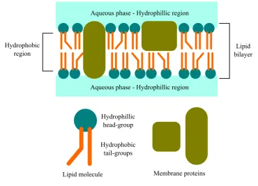
Studying the structure of membrane proteins
As well as polymers such as DNA and fibrous proteins, membrane proteins have also been studied with LD spectroscopy. Membrane proteins are biomolecules contained within the lipid bilayer membranes of cells. They are of significant interest because of the roles they play in a variety of processes in living things. These include cell signalling as apart of immune responses, control of substances entering and exiting a cell and monitoring and manipulating the shape of a cell. It is estimated that between 20% and 30% of the proteins in most organisms are membrane proteins. Furthermore, roughly 40% of drug targets are thought to be membrane proteins [9, 21, 47, 75, 103]. However, despite their importance, membrane proteins are difficult to study.
Aqueous phase - Hydrophillic region
Lipid bilayer
Aqueous phase - Hydrophillic region
Lipid molecule
Hydrophillic head-group
Hydrophobic tail-groups
Membrane proteins Hydrophobic
[image:45.595.141.512.86.353.2]region
Figure 1.7:Illustration of the basic components of phospholipids and a schematic cross-section of a phos-pholipid bilayer with membrane proteins.
of the lipid bilayer. They therefore cannot be treated in the same way that other proteins, such as F-actin, are by studying them in aqueous solutions. Membrane proteins are also very sensitive to other features of their environment, such as pH, and changes in these factors will lead to structural changes in the protein. This means that the protein structure observed after extraction and purification may not reflect its native structure in the cell membrane. Proteins can be extracted from membranes with the use of detergents and studies suggest that they are likely to retain structural features in the process. However, protocols for the extraction and purification of these proteins from the detergent are non-trivial [20, 21, 126].
secondary structure can be determined. However, it does not provide information about the location of these sub-structures within the protein [97].
A technique that can resolve the molecular detail of proteins more thoroughly is X-ray crystallography. This involves the formation of crystals made up of the protein. X-rays are then passed through the crystals to give a diffraction pattern. This pattern provides information about the relative location of atoms within a protein molecule [30]. While this technique has proven to be effective at elucidating the molecular structure of some proteins, the major bottleneck is the formation of crystals, and membrane proteins are notoriously difficult to crystallise [20]. Nuclear magnetic resonance (NMR) spectroscopy is an alternative technique that uses the magnetic properties of the nuclei of specific ele-ments to generate structural information about a molecule. This technique has been used to derive the structure of roughly 80 membrane proteins, and has also been used to obtain information about the motions of and interactions between substructures within a protein. This technique is limited by the large size of membrane proteins, though recent work has shown that structural studies of membrane proteins as large as 30–50 kDa are possible with NMR [62]. Furthermore, the sensitivity of membrane proteins to their environment means that the preparation of samples for NMR spectroscopy is a major factor in per-forming such a structural study.
1.5
Aligning vesicles in fluid flow
As previously mentioned, molecular alignment is crucial in LD spectroscopy. The exam-ples mentioned above refer to two different alignment methods: using a gel squeeze and using shear flow to align vesicles with membranes containing the protein of interest. This thesis shall focus on vesicles in fluid flows.
[image:49.595.194.456.301.529.2]Lipid vesicles can be categorised according to their size and lamellarity (if a vesicle is con-tained within a larger vesicle). The main categories, shown in Figure 1.9, are small unil-amellar vesicles (SUVs), medium unilunil-amellar vesicles (MUVs), large unilunil-amellar vesicles (LUVs), giant unilamellar vesicles (GUVs) and multilamellar vesicles (MLVs) [55, 79].
Figure 1.9: Vesicle types based on diameter and lamellarity. This diagram is reproduced with permission from the Figure 2 of [55].
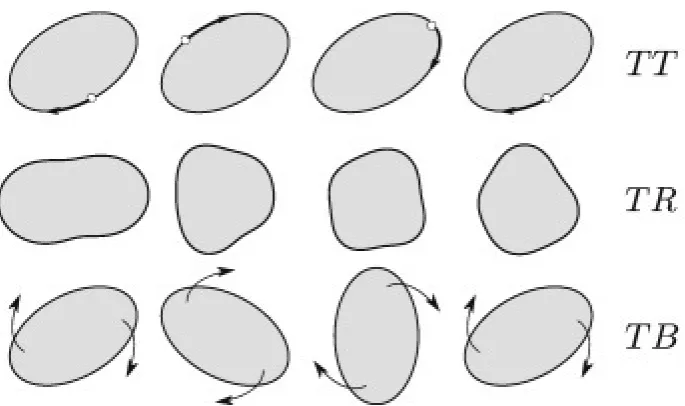
Figure 1.10:An illustration of the three types of behaviour that vesicles undergo in planar fluid-flow. The three lines corresponds with (from top to bottom) tank-treading (TT), trembling (TR) and tumbling (TB). These diagrams are reproduced with permission from the abstract figure of [2].
GUVs. Abreu et al. [2] published a review summarising this research, and the reader is asked to consult their work for full details. This section focuses on some of the major concepts discussed in the review paper.
In planar fluid flows, the three vesicle behaviours that are observed in fluid flows restricted to one plane are:
• Tank-treading, where the membrane rotates around the fluid bulk and the vesicle maintains the same angle with respect to the external environment.
• Tumbling, where the whole vesicle body rotates around its centre.
• Trembling, where the vesicle membrane fluctuates in an uncontrolled way.
These are illustrated in Figure 1.10. These three behaviours have been shown to take place in experimental conditions [2, 26, 58, 64, 76], but there have also been studies published to develop the theory behind what causes these three behaviours. The three main parameters that are thought to play a role in a vesicle’s behaviour in planar flows are:
• Theexcess area, ∆, corresponding to the deformation and stretching of the vesicle membrane in flow. This is defined by:
∆ = A
whereAis the surface area of the vesicle andR0is theeffective radiusof the vesicle, given by
R0 = 3V 4π
!1/3
. (1.5.2)
i.e. the vesicle’s effective radius is the radius of a sphere with the volume of the vesicle.
• Theviscosity contrast,λ, equal to the ratio of the fluid viscosities inside and outside the vesicle, denotedηi andηorespectively.
λ= ηi
ηo
= Fluid viscosity inside the vesicle
Fluid viscosity outside the vesicle. (1.5.3)
• In the case of linear shear flows, thecapillary number, defined by
Ca= γη˙ oR 3 0
κ , (1.5.4)
where ˙γ is the shear rate, ηo is the viscosity of fluid outside the vesicle, R0 is the effective radius as given by Equation (1.5.2) andκis themembrane bending energy. This is a dimensionless number that characterises the ease with which the viscous forces of the surrounding fluid will overcome the rigidity of the vesicle membrane to alter the vesicle shape. As an example, let: ˙γ = 1900 s−1, as in the case of the Couette flow cell described above; ηo = 8.9×10⁻⁴kg m−1s−1, the dynamic viscosity of water at 25◦C;
• R0 = 50 nm, the radius of a vesicle typically studied in CD and LD experiments; and
• κ ≈ 25kBT, as suggested by Abreu et al. [2], with kB = 1.38×10⁻²³J K−1 as Boltzmann’s constant and T = 298 K. In this instance, the capillary number is Ca= 0.0021.
Figure 1.11:A diagram illustrating the rotational (left) and extensional/elongational (right) components of a linear shear flow (middle). Reproduced from Figure 2 of [2].
Mathematically, the relationship between the fluid velocity vector,v, and the parameters
ωandsis given by
v= s(yex−xey)+ω(yex+ xey),
whereexandeyare the basis vectors for thex- andy-axes respectively. If these are equal, the result is a linear shear flow, andω = s = γ/˙ 2. For more general planar fluid flows,ω and s, the parameters corresponding to the extensional and rotational components of the flow, are considered instead of ˙γ.
The exact details of the parameter values at which changes between the three different vesicle behaviours occur have been the subject of debate in the literature. A number of theoretical models suggest that three main parameters are required to plot the phase diagram between all the vesicle behaviours [11, 25, 34, 61, 166, 167]. However Lebedev et al. [71] postulated that the vesicle behaviour can be deduced by calculating the value of two parameters: S (not connected with the orientation parameter S used in the LD literature) andΛdefined below.
S = 14π 3√3
ηoR30
κ∆ s, Λ =
23λ+32 24
! r
3∆ 10π
ω
s, (1.5.5)
where:
• R0is the effective radius (Equation (1.5.2)).
• ∆is the excess area (Equation (1.5.1)).
Figure 1.12: Phase diagram illustrating the regions of (S,Λ)-parameter space that correspond to the dif-ferent vesicle behaviours. Tank-treading takes place in the blue and green regions, trembling in the area between solid red and broken blue lines and tumbling in the orange and grey areas. The diagram is repro-duced from Figure 9 of [71].
• ηois the viscosities of the fluid outside the vesicle.
• λis the viscosity contrast (Equation (1.5.3)).
• ωandscorrespond to the extensional and rotational components of velocity of the surrounding fluid.
The associated phase diagram for the vesicle behaviour with respect to these two param-eters is shown in Figure 1.12. Experimental results suggest that this two-parameter setup is more closely followed by experimental results than the three-parameter setup proposed by other papers [2]. This setup is therefore considered in more detail below.
Spherical
Elongated
Figure 1.13: The elongation of a vesicle containing chromophores of interest in its membrane results in a net orientation of chromophores. In this example, the spherical vesicle has chromophores (in red) distributed evenly throughout its membrane, and the net orientation of the chromophores is zero. Elongation results in more of these chromophores occupying the parts of the membrane along the long axis of the vesicle, so the net orientation of the chromophores is close to vertical.
distribution of chromophores in the vesicle membrane means that the alignment of these chromophores with respect to the flow direction is not a significant issue. The elonga-tion is essential for this; in a perfectly spherical vesicle with target membrane molecules randomly distributed throughout, there would be no net orientation of the chromophores. Vesicle elongation means that target molecules are more likely to be present in the mem-branes along the long axis of the vesicle than the short axis, leading to a net non-zero alignment of the molecules of concern (see Figure 1.13).
Since tank-treading is the most preferable vesicle behaviour for LD experiments, the phase diagram suggests that the main parameter of concern is Λ. In the experimental setup, the fluids inside and outside a vesicle (and, therefore, their viscosities) are the same, so we consider the case where the viscosity contrastλ= 1. Then,
Λ≈ 0.708× √
∆ω
s
Figure 1.14: An illustration of the tilt of a vesicle away from a stationary boundary wall while in fluid shear flow. The vesicle is experiencing a lift forceFli f t, whose magnitude is dependent upon the shear rate
˙
γ. This diagram is reproduced with permission from the abstract figure of [2].
vesicle is more easily deformed and the excess area is large, then the membrane is likely to wrinkle. Furthermore, when the extensional strain rate is above a critical threshold, the vesicle stretch out as if it were a polymer uncoiling [2, 59, 106, 153, 168]. Therefore, in LD experiments, it is important that the lipid chosen to make up the vesicles allows for some shape deformation, but not too much.
Microelectro-mechanical systems were first developed in the 1980s for a variety of diff er-ent purposes, including pressure sensors for automotive applications, chemical sensors, capacitors and vibration detectors [88, 144]. These devices also gave birth to the field of microfluidics, where devices could be used to study objects in fluid flows and con-trol chemical reactions at the “micro” scale, smaller than what was previously possible (so-called “lab on a chip” technology). Earlier devices were based upon materials such as silicon and glass, which, while fabrication protocols were well known, made devices expensive to make. However the advent of polymer plastics have made the manufacture of microfluidic devices a cheaper process.
While a variety of different materials have been considered for use in making microfluidic devices, including the use of Shrinky Dinks®toys [33, 42, 95], one of the most commonly used materials is polydimethylsiloxane (PDMS) [87, 88, 144]. The first reported use of this material for microfluidic devices was in 1998 by Duffy et al. [31]. Sealed flow channels can be constructed by treating PDMS with oxygen plasma to create a hydrophilic surface that can be stuck on to a glass slide with heat treatment [31, 65, 145]. The polymer is also transparent to electromagnetic radiation with wavelengths in the range 240 nm to 1100 nm [87]. This allows us to use devices made from PDMS for linear dichroism experiments. However, there are some drawbacks to its use. For example, PDMS is hydrophobic and is able to absorb hydrophobic molecules from sample fluids that pass through it [92, 151]. This particular drawback could be a problem with studies of vesicle membrane proteins or membrane-bound molecules, as these molecules already have an affinity for the hydrophobic enviroment within the lipid bilayer.
lithog-Figure 1.15:This diagram illustrates the cross-slot device used by Tanyeri et al. [147]. (a) A hydrodynamic trap is created by a planar extensional flow field at the junction of two perpendicular microchannels. (b) The velocity field (top) and the potential well (bottom) for a particle in the flow field at the microchannel junction. This diagram is reproduced with permission from Figure 1 of [147].
raphy. Extensional flows have also been studied with microfluidics. One such example is in work by Tanyeri et al. [147] who developed a particle trapping device using an ex-tensional flow and across-slot. This is where the fluid enters a central chamber through two opposing channels on one axis (the compressional axis), and fluid leaves through two opposing channels on a perpendicular axis (the extensional axis), as illustrated in Fig-ure 1.15). This device was used to trap objects of roughly 1µm in diameter in the central stagnation point, using active flow controls to adjust the fluid flow rates exiting the cross-slot. Without such controls, such a particle would escape due to Brownian motion and the flow of fluid along the extensional axis [147, 148]. Cross-slot devices have also been used to study the uncoiling and extension of DNA molecules [135] and the behaviour of vesicles in extensional flows [59].
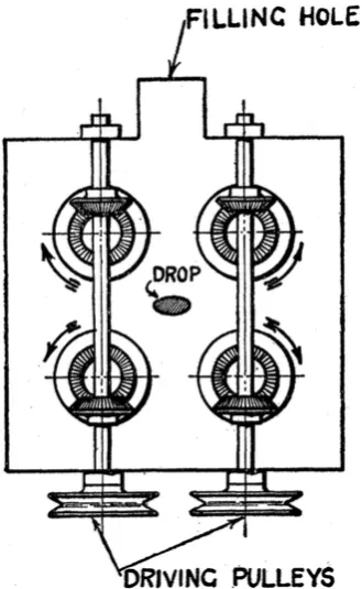
Figure 1.16: The four-roll mill device used by Taylor [150]. Four rotating mills controlled by driving pulleys cause the fluid drop in the centre to change shape. This diagram is reproduced with permission from Figure 1 of [150].
has been used to study the behaviour of vesicles in different planar fluid flows [26, 27, 76]. Of note is the work by Deschamps et al. [26], whose experimental results were shown to agree with the theoretical predictions established by Lebedev et al. [71].
It is again important to note that most of the studies considered here have used vesicles of at least 1µm in diameter, studied using microscopy. Vesicles in studies using LD have diameters of the order of 100 nm. The goal of this thesis is to establish whether such devices can be used for vesicle membrane protein studies with linear dichroism spec-troscopy and can achieve stronger LD signals through better alignment than possible with Couette flow. For extensional flow, the four-roll mill device would provide the exten-sional flows required for vesicle studies, but requires an extensive fluid pumping setup (Figure 1 in [76] provides an example of such a setup) that is beyond the scope of this project. Instead, an enhanced version of the cross-slot, as developed by Haward et al. [44] to optimize the area in the centre exposed to the greatest possible extensional strain, is used.
to run bead-spring simulations. Chapter 3 details the results from simulations, including comparisons with data reported by Hsieh et al. [48] to assess the performance of our code, and a test of the effect of hydrodynamic interactions on the alignment parameter value obtained.
Using FENE-Fraenkel springs in
polymer simulations
length, and where the tension force increases non-linearly as the spring length reaches this maximum permissible length.
Expressing this mathematically, let Qthe spring vector; this is a vector pointing in the same direction as the spring with length equal to the spring length, as illustrated in Fig-ure 2.1.
Q SpringVector
Figure 2.1:An illustration of a spring vector of a spring in a bead-spring chain.
The spring tension force,F, exerted by a FENE spring as a function of the spring vector Qis
F= HQ
1−QQ
max
2 (2.1.1)
where
• H > 0 is the spring constant.
• Q= |Q|is the length of the spring.
• Qmax >0 is the maximum length of the spring.


![Figure 1.9: Vesicle types based on diameter and lamellarity. This diagram is reproduced with permissionfrom the Figure 2 of [55].](https://thumb-us.123doks.com/thumbv2/123dok_us/9433641.449835/49.595.194.456.301.529/figure-vesicle-diameter-lamellarity-diagram-reproduced-permissionfrom-figure.webp)