A Local Meshless Method for Two Classes of Parabolic Inverse Problems

(1)

ISSN Print: 2327-4352

DOI: 10.4236/jamp.2018.65083 May 17, 2018 968 Journal of Applied Mathematics and Physics

A Local Meshless Method for Two Classes of

Parabolic Inverse Problems

Wei Liu, Baiyu Wang

*

College of Computer Engineering and Applied Mathematics, Changsha University, Changsha, China

Abstract

A local meshless method is applied to find the numerical solutions of two classes of inverse problems in parabolic equations. The problem is recon-structing the source term using a solution specified at some internal points; one class is that the source term is time dependent, and the other class is that the source term is time and space dependent. Some numerical experiments are presented and discussed.

Keywords

Meshless Method, Moving Least Squares, Local Radial Basis Functions, Inverse Problem, Parabolic Equation

1. Introduction

The inverse problem of parabolic equations appears naturally in a wide variety of physical and engineering settings; many researchers solved this problem using different methods [1]-[10]. An important class of inverse problem is recon-structing the source term in parabolic equation, and it has been discussed in many papers [11]-[19].

In meshless method, mesh generation on the spatial domain of the problem is not needed; this property is the main advantage of these techniques over the mesh dependent methods. The moving least squares method and the radial basis functions method are all the primary methods of constructing shape function in meshless method. The moving least squares method is introduced by Lancaster and Salkauskas [20] for the surface construction; in this method, one can obtain a best approximation in a weighted least squares sense, and this method empha-sizes the compacted support of weight function especially, so it has the local characteristics. The radial basis functions method [21] is very efficient

interpo-How to cite this paper: Liu, W. and Wang, B.Y. (2018) A Local Meshless Method for Two Classes of Parabolic Inverse Problems. Journal of Applied Mathematics and Phys-ics, 6, 968-978.

https://doi.org/10.4236/jamp.2018.65083

Received: March 29, 2018 Accepted: May 14, 2018 Published: May 17, 2018

(2)

DOI: 10.4236/jamp.2018.65083 969 Journal of Applied Mathematics and Physics lating technique related to the scattered data approximation, it has high preci-sion, and it is very suitable for the scattered data model; however, there are some drawbacks such as the character of global supported, the full matrix obtained from discretization scheme is always ill-conditioned as the number of colloca-tion points increases, and it is very sensitive for the seleccolloca-tion of the free parame-ter c.

To overcome the problems of ill-conditioned and the shape parameter sensi-tivity in radial basis functions method, the local radial basis function was intro-duced by Lee et al. [22]; in contrast to radial basis functions method, only scat-tered data in the neighboring points are used in local radial basis functions, in-stead of using all the points, thus the order of the matrix which is obtained from discretization being reduced, so the matrix of shape function is sparse. This will improve the computational accuracy and be suitable for solving large-scale problems [23].

The meshless method of moving least squares coupled with radial basis func-tions used for constructing shape function was introduced by Mohamed et al.

[24], but this method is global, and the problems in radial basis functions still exist. The method based on the linear combination of moving least squares and local radial basis functions in the same compact support was introduced by Wang [25], which is a local method, and is very suitable for practical prob-lems.

In this paper, we consider two classes of inverse problems of reconstructing the source term in parabolic equation from additional measurements, and we use the local meshless method presented in [25].

This paper is organized as follows. In Section 2, we give an outline of the local meshless method. In Section 3, we solve the inverse problems using the local meshless method. In order to illustrate the feasibility of the method, numerical experiments will be given in Section 4.

2. Preliminaries

Let Ω be an open bounded domain in Rd_{, given data values}

{

x uj, j

}

,j=1,2, , N, where

x

j is the distinct scattered point in Ω,

u

j is

the data value of function u at the node

x

j, N is the number of scattered nodes,

and we let u denote the approximate function of u in this work.

Combining with the collocation method, in [25], the approximate function

( )

u x _{was written as}

( )

1

, N

i i

i

u x ς x u

= =

∑

 (1)

where ςi

( )

x stands for the shape function, and it can be written as the linear

combination of the shape functions of moving least squares and local radial basis functions,

( )

M

( ) (

1

) ( )

L ,

i x i x i x

ς

=

νφ

+ −

ν ψ

( )

M

i x

φ

_and L

( )

i x

(3)

DOI: 10.4236/jamp.2018.65083 970 Journal of Applied Mathematics and Physics squares and local radial basis functions, respectively, ν is a constant which can be taken different values in [0, 1].

3. The Inverse Problem and Its Numerical Solution

Inverse problem I. The problem can be described as follows,

( )

2

( )

_{( )}

2

, ,

, 0 ,0 ,

u x t u x t

f t x l t T

t x

∂ ∂

= + < < < <

∂ ∂ (2)

with the initial condition

( )

,0 0

( )

, 0 ,

u x =u x < <x l (3) and the boundary conditions

( )

0, 1

( ) ( )

, , 2

( )

, 0 .

u t =u x u l t =u x ≤ ≤t T (4)

The Formulas (2)-(4) are the direct problem, and the inverse problem is that the functions u x t

( )

, and f t

( )

are unknown, with the additional observation of u x t

( )

, at some internal point x0

(

0<x0<l

)

,

(

0,

)

( )

,

u x t =E t (5)

according to (5), consider the following transformation in [26],

( )

2

(

0

)

( )

2

,

u x t

E t f t

x ∂

′ = +

∂ (6)

using (6), we get

( )

2

(

0

)

2

, ,

u x t

f t E t

x ∂ ′

= −

∂ (7)

substituting (7) into (2), we have

( )

2

( )

_{( )}

2

(

)

0

2 2

,

, ,

, 0 , 0 ,

u x t

u x t u x t

E t x l t T

t x x

∂

∂ ∂

′

= + − < < < <

∂ ∂ ∂ (8)

the initial and boundary conditions are

( )

,0 0

( )

, 0 ,

u x =u x < <x l (9)

( )

0, 1

( ) ( )

, , 2

( )

, 0 .

u t =u x u l t =u x ≤ ≤t T ₍₁₀₎ So the inverse problem is transformed to a direct problem, then we use the local meshless method described in Section 2 solving the problem (8)-(10).

From (1), the approximate function u x t

( )

, of u x t

( )

, at t t= m can be

represented as

(

)

( )

(

)

1

, m N j j m, ,

j

u x t ς x u x t

=

∑

  (11)

where ςj

( )

x is the shape function described in Section 2.

Then

(

)

2

( )

₍

₎

(

)

2

( )

₍

₎

2 2

0 0

2 2 2 2

1 1

, ,

, , , ,

N N

j j

m m

j m j m

j j

x x

u x t u x t

x x x x

ς ς

= =

∂ ∂

= =

∂

∑

∂  ∂

∑

∂ 

(4)

DOI: 10.4236/jamp.2018.65083 971 Journal of Applied Mathematics and Physics

1 , 1,2, ,

m m

t t + t m M

∆ = − =  , then we have

(

,m

)

(

, m1

) (

,m

)

_,

_{( )}

( )

m1

( )

m _, m

u x t u x t u x t E t E t E t

t t t

+ + ∂ − − ′ = = ∂ ∆ ∆  

so the Equation (8) can be rewritten as

(

) (

)

(

)

( )

(

)

1 2 2 0 1 2 2 1 1 , , ( ) , , , m m N N

j m m j

j m j m

j j

u x t u x t t

x E t E t x

u x t u x t

t x x ς ς + + = = − ∆ ∂ + ∂ = + − ∆ ∂ ∂

∑

   

that is equivalent to

(

)

(

)

( )

(

)

( )

(

)

2 1 1 2 1 2 0 2 1 , , , ( ) , , N

j m m

m m j m

j

N _j

j m j

x E t E t u x t u x t t u x t

t x

x

u x t x ς ς + + = =  ∂ − = + ∆ _ + ∆ ∂   ∂ − _ ∂ _

∑

   

by substituting each xk for x,

(

)

(

)

( )

(

)

( )

₍

₎

2 1 1 2 1 2 0 2 1 , , , , , N

j k m m

k m k m j m

j

N _j

j m j

x E t E t u x t u x t t u x t

t x

x

u x t x ς ς + + = =  ∂ − = + ∆ _ + ∆ ∂   ∂ − _ ∂ _

∑

    (12)

from (12) and the conditions (9)-(10), we can obtain the numerical solution

(

k m,

)

u x t , and f t

( )

m ,k=1,2, , , N m=1,2, , M.

Inverse problem II. The problem can be described as follows,

( )

2

( )

_{( )}

2

, ,

, , 0 ,0 ,

u x t u x t

f x t x l t T

t x

∂ ∂

= + < < < <

∂ ∂ (13)

with the initial condition

( )

,0 0

( )

, 0 ,

u x =u x < <x l (14)

and the boundary conditions

( )

0, 0,

( )

, 0, 0 .

u t = u l t = ≤ ≤t T (15)

The Formulas (13)-(15) are the direct problem, and the inverse problem is that the functions u x t

( )

, and f x t

( )

, are unknown, with the additional ob-servation of u x t

( )

, at some internal point x0

(

0<x0<l

)

,

(

0,

)

( )

.

u x t =E t (16) Assume that the function f x t

( )

, can be described as

( ) ( ) ( )

, ,

f x t =η ψt x (17) where ψ

( )

x is the known function, and satisfies the following restrictions:

1) ψ

( )

x0 ≠0,

2) ψ

( )

x _{is smooth enough,}

(5)

DOI: 10.4236/jamp.2018.65083 972 Journal of Applied Mathematics and Physics Let

( )

,

( ) ( )

( )

, ,

u x t =θ t ψ x +ω x t (18)

where

( )

t ₀t

( )

s sd ,

θ

=

_∫

η

(19)

substituting (17) and (18) into (13), we have

( )

2

( )

_{( )}

2

( )

2 2

, , d

, 0 ,0 ,

d

x t x t x

t x l t T

t x x

ω ω ψ

θ

∂ ∂

= + < < < <

∂ ∂ (20)

from (18) and combining (16),we get

( )

_{( )}

(

0

)

0

, ,

E t x t

t

x ω θ

ψ −

= (21)

then according to (19),

( )

t

( )

t ,

η =θ′ ₍₂₂₎

substituting (21) into (20),

( )

(

)

( )

2 2

0

2 2

0

,

, , d

, 0 ,0 ,

d

E t x t

x t x t x

x l t T

t x x x

ω

ω ω ψ

ψ −

∂ ∂

= + < < < <

∂ ∂ (23)

the initial and boundary conditions are

( )

x,0 u x0

( )

, 0 x l,

ω = < < (24)

( )

0,t 0,

( )

l t, 0, 0 t T.

ω = ω = ≤ ≤ (25)

Through the above descriptions, if we have the numerical solution ω

( )

x t,

of (23), from (17)-(18) and (21)-(22), we can get the numerical solution u x t

( )

,

and f x t

( )

, .

Next, we use the local meshless method described in Section 2 solving the problem (23)-(25).

From (1), the approximate function ω

( )

x t, of ω

( )

x t, at t t= m can be

represented as

(

)

( )

(

)

1

, m N j j m, ,

j

x t x x t

ω ς ω

=

∑

 

where ςj

( )

x is the shape function described in Section 2.

Then

(

0

)

( )

0

(

)

22 2

( )

2

(

)

1 1

, N , , N j , ,

m j j m j m

j j

x

x t x x t x t

x x

ς ω

ω ς ω ω

= =

∂ ∂

= =

∂ ∂

∑



∑

  

for ∂_∂

ω

_t , we apply one step forward difference formula to t, and let

1 , 1,2, ,

m m

t t + t m M

∆ = − = _ _{, then we have}

(

x t,m1

)

(

x t, m

)

_,

t t

ω ω

ω + −

∂ =

∂ ∆

 

(6)

(

)

(

)

( )

₍

₎

( )

(

)

( )

1

2 0 2

1 2 2 1 0 , , , d , , d m m N

m j j m

N _j _j

j m j

x t x t

t

E t x x t

x x x t x x x ω ω ς ω ς ψ ω ψ + = = − ∆ − ∂ = + ∂

∑

   

that is equivalent to

(

)

(

)

( )

(

)

( )

(

)

( )

2 1 2 1 0 2 1 2 0 , , , , d , d N j

m m j m

j

N

m j j m

j

x

x t x t t x t

x

E t x x t

x

x x

ς

ω ω ω

ς ω ψ ψ + = =  ∂  = _{+∆ } ∂    − _  +   

∑

   

by substituting each xk for x,

(

)

(

)

( )

(

)

( )

(

)

( )

2 1 2 1 0 2 1 2 0 , , , , _d , d N j k

k m k m j m

j

N

m j j m

j k

x

x t x t t x t x

E t x x t

x

x x

ς

ω ω ω

ς ω _ψ

ψ + = =   ∂ = + ∆  ∂    − _  +   

∑

  

 (26)

from (26) and the conditions (24)-(25), we can obtain the numerical solution

(

x tk m,

)

ω and f x t

(

k m,

)

,k=1,2, , , N m=1,2, , M .

4. Numerical Experiments and Discussions

To test the efficiency of the method in this paper, in this section, we give two examples to illustrate the correctness of the theoretical result and the feasibility of the method.

Example 1. Consider the problem (2)-(5), with the conditions

( )

( ) (

)

( ) (

)

( )

0 2 sin , 0 2 e ,t 1 2 sin e ,t sin π ,

u x _{= +} x u t ₌ ₊t − u t ₌ _{+ +}t l − E t ₌ t

and we let l=2,T =2,x0=1.

The exact solutions are

( ) (

, 2 sin e ,

)

t

( ) (

1

)

e .t

u x t ₌ _{+ +}t x − f t _{= − +}t −

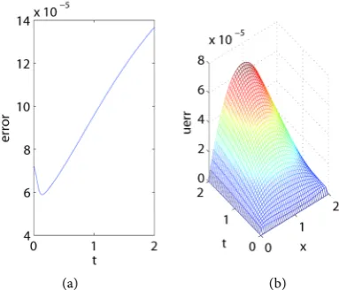
[image:6.595.206.536.72.414.2]

Firstly, we plot the error functions f t

( )

− f t

( )

_and u x t u x t

_{( ) ( )}

, − , in Figure 1, respectively, where ∆ =t 0.0001,∆ =x 0.05.

From Figure 1, we can see that the approximation effect is good.

(7)

[image:7.595.274.466.73.237.2]

(a) (b)

Figure 1. The error functions (a) f t

( )

− f t

( )

; (b) u x t u x t

( ) ( )

, − , .

( )

( )(

1

)

,

E tγ =E t +γ (27)

where γ is the noise parameter.

We plot the error functions f t

( )

−f t

( )

_and u x t u x t

( ) ( )

, − , when

0.001

γ = _{in Figure 2, where} ∆ =t 0.0001,∆ =x 0.05_.

From Figure 2, we see that when there is the noisy data, the approximation effect of numerical solution is worse relatively, but there is no obvious oscillation in the error graph.

Lastly, we define the following error of functions f t

( )

and u x t

( )

, ,

( ) ( )

(

)

2

(

( ) ( )

)

2

1 1 1

, ,

N M N

j j i j i j

j i j

f t f t u x t u x t

Ef Eu

N MN

= = =

− −

=

∑

=

∑∑

 _

(28)

where f t u x t

( ) ( )

j , i, j and f t u x t

( ) ( )

j , i, j are the exact and numerical

solu-tions at

x t

j m

,

, M and N are the number of nodes about x and t, respectively. we give the results under the different cases in Table 1.

From Table 1, we get that the error decreases with the decrease of Δt, when the number of nodes are fixed. When Δt is fixed, the error decreases with the in-crease of the number of nodes. When Δt and Δx are fixed, the error varies with the change of the noisy data, and the error decreases with the decrease of noisy data.

Example 2. Consider the problem (13)-(16), with the conditions

( )

0 0, sin π ,

u x = E t = t

and we let l=1,T =1,x0 =0.5.

The exact solutions are

( )

, sin π sin π ,

( ) ( ) ( )

πsin π

( )

(

cos π

( )

πsin π ,

( )

)

u x t = x t f t = x + t

with

( )

x πsin π .

( )

x

ψ =

(8)

[image:8.595.259.481.74.246.2]

(a) (b)

Figure 2. The error functions (a) f t

( )

− f t

( )

_{; (b)} u x t

( ) ( )

, −u x t , .

Table 1. The error under different cases.

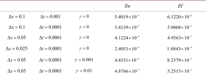
Eu Ef

0.1

x

∆ = ∆ =t 0.001 γ =0 _{3.0404 10}_× −4 _{8.9672 10}_× −4

0.1

x

∆ = ∆ =t 0.0001 γ =0 _{3.2054 10}_× −5 _{1.0005 10}_× −4

0.05

x

∆ = ∆ =t 0.0001 γ =0 _{3.0491 10}_× −5 _{9.9319 10}_× −5

0.05

x

∆ = ∆ =t 0.0001 γ =0.01 _{1.0624 10}_× −2 _{3.6728 10}_× −2

0.05

x

∆ = ∆ =t 0.0001 γ =0.001 _{1.0902 10}_× −3 _{3.7621 10}_× −3

0.05

x

∆ = ∆ =t 0.0001 γ =0.01 _{9.7477 10}_× −5 _{6.6848 10}_× −4

0.05

x

∆ = ∆ =t 0.0001 γ =0.001 _{2.8639 10}_× −5 _{6.7360 10}_× −4

functions f x t

( )

, − f x t

( )

, and u x t u x t

( ) ( )

, − , in Figure 3, where

0.0001, 0.05

t x

∆ = ∆ = .

From Figure 3, we see that the approximation effect is good.

Secondly, in order to test the stability of the numerical solution, we give small perturbations on E t

( )

, and the artificial error is defined by (27).

The results of f x t

( )

, −f x t

( )

, _and u x t u x t

( ) ( )

, − , with γ=0.001 are shown in Figure 4, where ∆ =t 0.0001,∆ =x 0.05_.

From Figure 4, we see that when there is noise, the approximation effect is worse than there is no noise, but the error function is smooth and there is no obvious oscillation in error graph.

At last, we define Eu by (28), and the definition of Ef is same as Eu, we give the results under the different cases in Table 2.

From Table 2, we get that when γ =0, the error decreases with the decrease of Δt and Δx, when Δt and Δx are fixed, the error decreases with the decrease of noise parameter.

5. Conclusion

[image:8.595.207.540.303.440.2]

(9)

[image:9.595.238.494.73.258.2]

(a) (b)

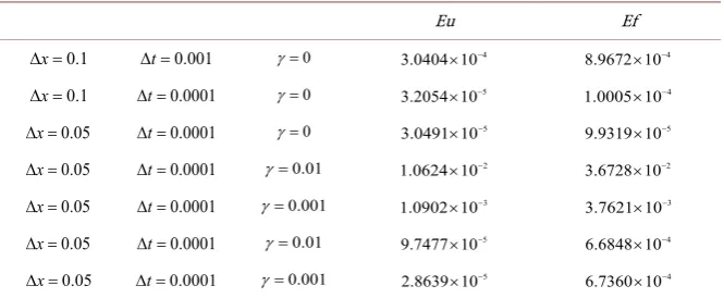
Figure 3. The error functions (a) f x t

( )

, − f x t

( )

, ; (b) u x t u x t

( ) ( )

, − , .

[image:9.595.234.495.306.477.2]

(a) (b)

Figure 4. The error functions (a) f x t

( )

, − f x t

( )

, ; (b) u x t u x t

( ) ( )

, − , .

Table 2. The error under different cases.

Eu Ef

0.1

x

∆ = ∆ =t 0.001 γ =0 _{5.4019 10}_× −5 _{6.1220 10}_× −2

0.1

x

∆ = ∆ =t 0.0001 γ =0 _{3.4139 10}_× −5 _{5.0868 10}_× −2

0.05

x

∆ = ∆ =t 0.0001 γ =0 _{4.1224 10}_× −6 _{4.9563 10}_× −3

0.025

x

∆ = ∆ =t 0.0001 γ =0 _{2.4053 10}_× −6 _{1.8843 10}_× −4

0.05

x

∆ = ∆ =t 0.0001 γ =0.001 _{4.8531 10}_× −4 _{8.2379 10}_× −3

0.05

x

∆ = ∆ =t 0.0001 γ =0.01 _{4.8766 10}_× −3 _{5.2515 10}_× −2

[image:9.595.207.540.534.657.2]

(10)

Acknowledgements

This work was supported by Scientific Research Fund of Scientific and Technol-ogical Project of Changsha City, (Grant No. ZD1601077, K1705078).

References

[1] Liu, Z.H. and Wang, B.Y. (2009) Coefficient Identification in Parabolic Equations. Applied Mathematics and Computation, 209, 379-390.

https://doi.org/10.1016/j.amc.2008.12.062

[2] Liu, J.B., Wang, B.Y. and Liu, Z.H. (2010) Determination of a Source Term in a Heat Equation. International Journal of Computer Mathematics, 87, 969-975.

https://doi.org/10.1080/00207160802044126

[3] Hasanov, A. and Liu, Z.H. (2008) An Inverse Coefficient Problem for a Nonlinear Parabolic Variational Inequality. Applied Mathematics Letters, 21, 563-570.

https://doi.org/10.1016/j.aml.2007.06.007

[4] Liu, Z.H. and Tatar, S. (2012) Analytical Solutions of a Class of Inverse Coefficient Problems. Applied Mathematics Letters, 25, 2391-2395.

https://doi.org/10.1016/j.aml.2012.07.010

[5] Wang, B.Y. (2014) Moving Least Squares Method for a One-Dimensional Parabolic Inverse Problem. Abstract and Applied Analysis, 2014, Article ID 686020, 12 pages. [6] Fatullayev, A.G. (2002) Numerical Solution of the Inverse Problem of Determining

an Unknown Source Term in a Heat Equation. Mathematics and Computers in Si-mulation, 58, 247-253.https://doi.org/10.1016/S0378-4754(01)00365-2

[7] Badia, A.E. and Duong, T.H. (2002) An Inverse Problem in Heat Equation and Ap-plication to Pollution Problem. Journal of Inverse and Ill-posed Problems, 10, 585-599.https://doi.org/10.1515/jiip.2002.10.6.585

[8] Cannon, J.R. (1968) Determination of an Unknown Heat Source from Overspeci-fied Boundary Data. SIAM Journal on Numerical Analysis, 5, 275-286.

https://doi.org/10.1137/0705024

[9] Choulli, M. and Yamamoto, M. (2004) Conditional Stability in Determining a Heat Source. Journal of Inverse and Ill-Posed Problems, 12, 233-243.

https://doi.org/10.1515/1569394042215856

[10] Hussein, M.S. and Lesnic, D. (2016) Simultaneous Determination of Time and Space-Dependent Coefficients in a Parabolic Equation. Communications in Nonli-near Science and Numerical Simulation, 33, 194-217.

https://doi.org/10.1016/j.cnsns.2015.09.008

[11] Cannon, J.R. and Lin, Y. (1990) An Inverse Problem of Finding a Parameter in a Semi-Linear Heat Equation. Journal of Mathematical Analysis and Applications, 145, 470-484.https://doi.org/10.1016/0022-247X(90)90414-B

[12] Cannon, J.R. and DuChateau, P. (1998) Structural Identification of an Unknown Source Term in a Heat Equation. Inverse Problems, 14, 535-551.

https://doi.org/10.1088/0266-5611/14/3/010

[13] Burykin, A.A. and Denisov, A.M. (1997) Determination of the Unknown Sources in the Heat-Conduction Equation. Computational Mathematics and Modeling, 8, 309-313.https://doi.org/10.1007/BF02404048

(11)

DOI: 10.4236/jamp.2018.65083 978 Journal of Applied Mathematics and Physics [15] Johansson, T. and Lesnic, D. (2007) Determination of a Spacewise Dependent Heat

Source. Journal of Computational and Applied Mathematics, 209, 66-80.

https://doi.org/10.1016/j.cam.2006.10.026

[16] Johansson, T. and Lesnic, D. (2007) A Variational Method for Identifying a Space-wise-Dependent Heat Source. IMA Journal of Applied Mathematics,72, 748-760.

https://doi.org/10.1093/imamat/hxm024

[17] Fatullayev, A.G. and Can, E. (2000) Numerical Procedures for Determining Un-known Source Parameters in Parabolic Equations. Mathematics and Computers in Simulation,54, 159-167.https://doi.org/10.1016/S0378-4754(00)00221-4

[18] Borukhou, V.T. and Vabishchevich, P.N. (2000) Numerical Solution of the Inverse Problem of Reconstructing a Distributed Right-Hand Side of a Parabolic Equation. Computer Physics Communications, 126, 32-36.

https://doi.org/10.1016/S0010-4655(99)00416-6

[19] Saadatmandi, A. and Dehghan, M. (2010) Computation of Two-Dependent Coeffi-cients in a Parabolic Partial Differential Equation Subject to Additional Specifica-tions. International Journal of Computer Mathematics, 87, 997-1008.

[20] Lancaster, P. and Salkauskas, K. (1981) Surfaces Generated by Moving Least Squares Methods. Mathematics of Computation,37, 141-158.

https://doi.org/10.1090/S0025-5718-1981-0616367-1

[21] Buhmann, M.D. (2003) Radial Basis Functions: Theory and Implementations. Cambridge University Press, Cambridge.

https://doi.org/10.1017/CBO9780511543241

[22] Lee, C.K., Liu, X. and Fan, S.C. (2003) Local Multiquadric Approximation for Solv-ing Boundary Value Problems. Computational Mechanics,30, 395-409.

https://doi.org/10.1007/s00466-003-0416-5

[23] Li, M., Chen, W. and Chen, C.S. (2013) The Localized RBFs Collocation Methods for Solving High Dimensional PDEs. Engineering Analysis with Boundary Ele-ments, 37, 1300-1304.https://doi.org/10.1016/j.enganabound.2013.06.001

[24] Mohamed, H.A., Bakrey, A.E. and Ahmed, S.G. (2012) A Collocation Mesh-Free Method Based on Multiple Basis Functions. Engineering Analysis with Boundary Elements, 36, 446-450.https://doi.org/10.1016/j.enganabound.2011.09.002

[25] Wang, B. (2015) A Local Meshless Method Based on Moving Least Squares and Lo-cal Radial Basis Functions. Engineering Analysis with Boundary Elements, 50, 395-401.https://doi.org/10.1016/j.enganabound.2014.10.001