Energy Efficient Hierarchical Stable Election Protocol
L. Jagadeesh Naik
Dept of ECE, BIT IT-Hindupur, Anantapur Dt. IndiaK. V. Ramanaiah, PhD
Professor, Dept of ECE, Y.S.R.Engg. College, YogivemanaUniversity-Proddutur
K. Soundara Rajan, PhD
Professor,Dept of ECE, J.N.T.U. Anantapur, India
ABSTRACT
In the energy efficient routing protocols clustering is done as uniformly and select as cluster head (CH) based on remaining energy and distance of the nodes. This protocol is modification of SEP protocol. The election of Cluster Head (CH) in EEHSEP protocol is based on remaining energy and best node with respect to distance between other nodes and sink node. The energy consumption of sensor nodes is based on the distance traveled by packet, if node transmits loner distance it consume more energy than shorter distance. In this protocol obtains distance between nodes is using distance equation formula. It is calculate distance between node and obtained average distance from the cluster head, based on best average distance of nodes select cluster head.
Keywords
WSN, SEP, Routing
1.
INTRODUCTION
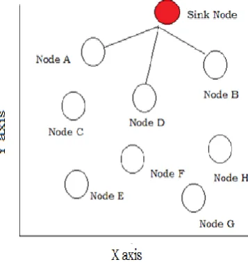
In this section describes distance calculation in EEHSEP protocol Let consider two sensor nodes (node A and node B) and sink node with specific characteristic obtaining for other sensor nodes position in the network, the nodes simultaneously sending signal to sink node, node A. These nodes are directly received signal obtain distance between these three points. The table consists of information of sink node, sensor node A, sensor node B and all other sensor nodes. The fields in the table are having distance between nodes and number of nodes etc. according field in table node A and node B obtain of distance to each other nodes. These fields information is send to sink node and all other nodes for updating information[1-2]. The sink node fields in table as shown in below table 1.1
Table 1: Nodes Information in network
xj, yj Sensor nodes Coordinate
Mj Sensor node number
di,j Distance between node mi and node mj
Cj Sink Node distance
aj Node A distance
bj Node B distance
[image:1.595.316.546.203.413.2]O.5 Optimal probability (Popt)
Fig. 1.1: An example of clustering of nodes in EEHSEP
Find out of every nodes characteristic; Let an example compute sensor node D characteristic as shown in Figure 1.2. Let assume that attribute of each node such as Node A= , Node B = and base station/sink node= .
[image:1.595.337.516.499.688.2]To obtain characteristics of the sensor node D with distance from nodes such as Node A, Node B and base station are certain amount of a, b, c.
Let assume that node D characteristic is D = (x4, y4). According to the formula calculates distance from node D to sink node is given equation 1.
Similarly below equations 2 and 3
(3)
To obtain equation subtracted equation 2 from equation 3 the equal to equation 4.
To replacing with quantity of in equation 1, after setting coefficients of equal power, solve between two points
[image:2.595.119.489.291.610.2]which as marked. These are replaced with in equation 1, these calculations have been done for all sensor nodes in the network, base station and each sensor node of characteristics are saved in the table 5.1 by using these nodes characteristic should determine distance of each node from every other nodes. Remaining other node characteristic also saved to similar table, and then, compared with nodes in network area and the sensors nodes are divided into equal area (cluster) in a network. This is form as clusters. The cluster sensor node is in specific condition. These sensor nodes may be in vertical line, horizontal line or both of them. Let assume that they are three conditions: first condition if node is coming towards horizontal line, assume that it is a bottom square member. Second condition if node is coming towards vertical line, assume that it is left square member. Finally if node coming towards both horizontal and vertical lines, assume that it is bottom square member. Accordingly all sensors nodes in the network will be a member of one square area, assume that every square area should be a cluster, in each cluster should be select cluster head[5].
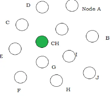
Figure 3: Selection of Cluster Head
To election of cluster head will get the probability of cluster head based on remaining energy and average distance of each node in the network. To obtain average distance of each node from each other nodes in same cluster and put average distance into the equation 6, and also obtain remaining energy of each the node[4]. For example find cluster head in figure 3.
(5)
Where average distance (6)
m is No of sensor nodes in cluster
mi= ith Node
= distance between WSN nodes
is energy remaining of each WSN node
(CH) for clusters.
2.
EEHSEP PROTOCOL
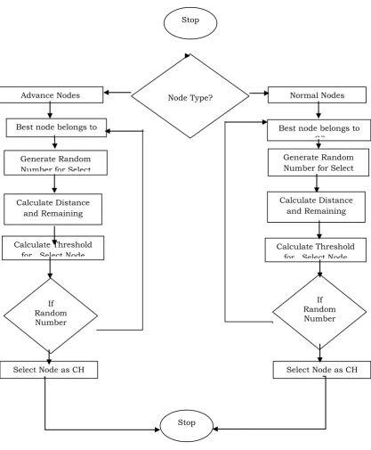
[image:3.595.93.511.158.664.2]The main object of this proposed approach is to enhance the life time of wireless sensor networks by ensuring uniform allocation of sensor nodes in the clusters, hence there is not much overhead for packets transmitting and receiving on Cluster Heads.
Figure 4: Flow chat for Cluster Head Selection
Normal Nodes Advance Nodes
Best node belongs to G’
Generate Random Number for Select
Node
Best node belongs to G’’
Generate Random Number for Select
Node
Calculate Threshold
for Select Node Calculate Threshold for Select Node
Select Node as CH If Random Number < TAdv
If Random Number < Tnor
Select Node as CH Calculate Distance
and Remaining Energy
Calculate Distance and Remaining
Energy
Stop Node Type?
3.
RESULTS AND DISCUSSIONS
[image:4.595.312.545.71.286.2]The simulation results of SEP, EEHSEP protocols have been carried out by using network simulator (NS 2.35). The simulation results were obtained by varying No. of nodes. The following simulation scenario table 2 used for obtaining results.
Table: 2. Simulation parameter
Scenario parameter Value Routing Protocols SEP, EEHSEP
Number of Nodes 50,60,70,80,90,100
EO 10 J
Simulation area 1000×1000 sq. M
Popt 0.5
Data Rate 1 Mbps
Simulation time 100 sec
EO 10 J
Antenna Omni Directional
Figure 5. Energy Consumption
Figure 5 shows that energy consumptions of SEP, EEHSEP protocols by varying number of nodes. The EEHSEP is less energy consumption than SEP protocol. The cluster head (CH) are symmetrically selected based on remaining energy and distance between nodes and sink node, the EEHSEP protocol has more energy efficient.
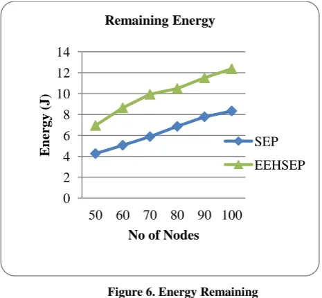
Figure 6. Energy Remaining
[image:4.595.53.296.146.533.2]The remaining energy is obtain in SEP, EEHSEP by varying no of nodes. The remaining energy of EEHSEP is higher than SEP as shown in above figure 6. The remaining energy is high in EEHSEP protocol because of cluster head selected with best distance of sink node and as well as other nodes.
Figure 7. Packet Delivery Ratio
The EEHSEP protocol has higher packet delivery ratio when compare with SEP protocols as shown in above figure 7. The PDR is slightly decreased with increasing number of nodes
0 2 4 6 8 10 12 14 16 18
50 60 70 80 90 100
E
nerg
y
(J
)
No of nodes
Energy consumed
SEP
EEHSEP
0 2 4 6 8 10 12 14
50 60 70 80 90 100
E
nerg
y
(
J
)
No of Nodes Remaining Energy
SEP
EEHSEP
0 20 40 60 80 100 120
50 60 70 80 90 100
P
DR
No of Nodes Packet Delivery Ratio
SEP
[image:4.595.371.520.352.555.2]Figure 8. End to End Delay
[image:5.595.346.568.72.285.2]From the figure end delay is increased with increasing nodes. Obtained end to end delay for EEHSEP, SEP protocols by varying No. of nodes i.e. from 50 to 100 nodes and node speed constant. The EEHSEP protocol is has less delay when compare with SEP protocols as shown in figure 8.
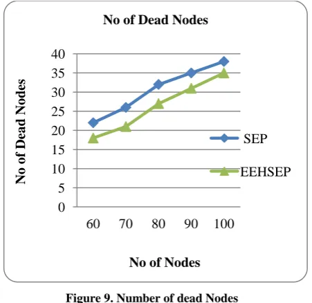
Figure 9. Number of dead Nodes
The number of dead nodes increases with increasing no of nodes as shown in figure 9. The number of dead nodes are less in EEHSEP when compare with SEP.
Figure.10. Overhead Vs No of Nodes
From the Figure 10 illustrate that, overhead increases with varying number of nodes. The EEHSEP protocol has higher overhead when compared with SEP protocols as shown in figure 10. In the EEHSEP protocol overhead increases due to calculation of distance between nodes and to maintain nodes characteristics information in the network.
4.
CONCLUSION
In this paper simulation of proposed EEHSEP protocols is carried out using network simulator (ns 2. 35). The EEHSEP protocol given better performance when compare with SEP protocol.The energy consumption decreases by 12% than SEP protocol, the packet delivery ratio also increase by 9%. The EEHSEP Protocol gives better performance interns of no of dead nodes but overhead of the networks is high compare with SEP protocols.
5.
REFERENCES
[1] K. Cohen and A. Leshem, “Density-based multiple access for detection in wireless sensor networks,” in IEEE International Symposium on Information Theory (ISIT), pp. 776–780, June 2018
[2] T. Sujithra, N. S. Kumar, K. K. Kumar, and V. Vinayagam, “Survey on data gathering approaches in wireless sensor networks,” Indian Journal of Science and Technology, vol. 10, no. 25, 2017.
[3] K. Cohen and Q. Zhao, “Active hypothesis testing for anomaly detection,” IEEE Transactions on Information Theory, vol. 61, no. 3, pp. 1432–1450, 2015.
[4] K. Cohen and Q. Zhao, “Asymptotically optimal anomaly detection via sequential testing,” IEEE Transactions on Signal Processing, vol. 63, no. 11, pp. 2929–2941, 2015. [3] S. Faisal, N. Javaid, A. Javaid, M. A. Khan, S. H. Bouk and Z. A. Khan, "Z-SEP: Zonal-Stable Election Protocol for Wireless Sensor Networks" Journal of Basic and Applied Scientific Research (JBASR), 2013.
[5] H. Kour and A. K. Sharma, “Hybrid Energy Efficient Distributed Protocol for Heterogeneous Wireless Sensor Network,” International Journal of Computer Applications Vol. 4, No.6, July 2010.
[6] Laveena Mahajan, Narinder Shanna “Improving the
50 60 70 80 90 100
E nd t o E nd Dela y ( s)
No of Nodes End to End Delay
SEP EEHSEP 0 5 10 15 20 25 30 35 40
60 70 80 90 100
No o f Dea d No des
No of Nodes No of Dead Nodes
SEP EEHSEP 0 500 1000 1500 2000 2500 3000
50 60 70 80 90 100
O
v
erhea
d
Number of nodes Overhead
SEP
[image:5.595.59.285.366.585.2]Stable Period of WSN using Dynamic Stable Leach Election Protocol” 2014 International Conference on Issues and Challenges in Intelligent Computing Techniques (ICICT), pp. 393-401, 2014
[7] Arafat Abu Malluh, Khaled M. Elleithy, Zakariya Qawaqneh, Ramadhan J. Mstafa, Adwan Alanazi “EM-SEP: An Efficient Modified Stable Election Protocol”, Proceedings of 2014 Zone 1 Conference of the American Society for Engineering Education (ASEE Zone1). 2014 [8] Dahlila P. Dahnil, Yaswant P. Singh, Chin Kuan Ho
“Energy-Efficient Cluster Formation in Heterogeneous Wireless Sensor Networks: A Comparative Study” ICACT2011, pp no. 746-751, Feb. 13-16, 2011.
[9] O. Rehman, N. Javaid, B. Manzoor, A. Hafeez, A. Iqbal, M. Ishfaq “Energy Consumption Rate based Stable Election Protocol (ECRSEP) for WSNs” Procedia Computer Science 19 ( 2013 ) 932 – 937.
[10] Mritunjay Rai,Shekhar Verma,Shashikala Tapaswi.A Power Aware Minimum Connected Dominating Set for Wireless Sensor Networks.Journal of networks, VOL. 4, NO. 6, AUGUST 2009.
[11]Weili Wua,Hongwei Dub,Xiaohua Jia, Yingshu Li, Scott C.-H. Huang.Minimum connected dominating sets and
maximal independent sets in unit disk graphs.Theoretical Computer Science 352 (2006) 1 7.
[12] Gao, J., Guibas, L., Hershberger, J., Zhang, L., Zhu, A.Discrete mobile centers.17th Annual Symposium on Computational 196. ACM Press, New York (2001) [13] Luby, M.A simple parallel algorithm for the maximal
independent set problem.17th Annual ACM Symposium on Theory of 10. ACM Press, New York (1985).
[14] Amitabha Bagchi, Sparse power-efficient topologies for wireless ad hoc sensor networks, IEEE International Symposium on Parallel and Distributed Systems, 19-23 April, 2010,
[15] Sohrabi, K., Gao, J., Ailawadhi, V., Pottie, G., “Protocols for Self-Organization of a Wireless Sensor Network,” IEEE Personal Communications Mag., Vol.7, No.5, pp.16-27, Oct. 2000.