Least Squares Method from the View Point of Deep Learning

(1)

ISSN Online: 2160-0384 ISSN Print: 2160-0368

DOI: 10.4236/apm.2018.85027 May 29, 2018 485 Advances in Pure Mathematics

Least Squares Method from the View Point of

Deep Learning

Kazuyuki Fujii

1,2

1_{International College of Arts and Sciences, Yokohama City University, Yokohama, Japan,} 2_{Department of Mathematical Sciences, Shibaura Institute of Technology, Saitama, Japan}

Abstract

The least squares method is one of the most fundamental methods in Statistics to estimate correlations among various data. On the other hand, Deep Learn-ing is the heart of Artificial Intelligence and it is a learnLearn-ing method based on the least squares. In this paper we reconsider the least squares method from the view point of Deep Learning and we carry out the computation thorough-ly for the gradient descent sequence in a very simple setting. Depending on the values of the learning rate, an essential parameter of Deep Learning, the least squares methods of Statistics and Deep Learning reveal an interesting difference.

Keywords

Least Squares Method, Statistics, Deep Learning, Learning Rate, Linear Algebra

1. Introduction

The least squares method in Statistics plays an important role in almost all dis-ciplines, from Natural Science to Social Science. When we want to find proper-ties, tendencies or correlations hidden in huge and complicated data we usually employ the method. See for example [1].

On the other hand, Deep Learning is the heart of Artificial Intelligence and will become a most important field in Data Science in the near future. As to Deep Learning see for example [2][3][4][5][6].

Deep Learning may be stated as a successive learning method based on the least squares method. Therefore, to reconsider it from the view point of Deep Learning is very natural and we carry out the calculation thoroughly of the suc-cessive approximation called gradient descent sequence.

How to cite this paper: Fujii, K. (2018) Least Squares Method from the View Point

of Deep Learning. Advances in Pure

Ma-thematics, 8, 485-493.

https://doi.org/10.4236/apm.2018.85027

Received: April 10, 2018 Accepted: May 26, 2018 Published: May 29, 2018

(2)

DOI: 10.4236/apm.2018.85027 486 Advances in Pure Mathematics When the learning rate changes a difference in method between Statistics and Deep Learning gives different results.

Theorem I and II in the text are our main results and a related problem (exer-cise) is presented for readers. Our results may give a new insight to both Statis-tics and Data Science.

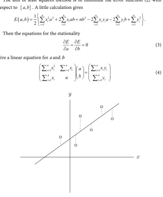
First of all let us explain the least squares method for readers in a very simple setting. For n pieces of two dimensional real data

(

) (

)

(

)

{

x y1, 1 , x y2, 2 , , x yn, n

}

we assume that their scatter plot is like Figure 1

Then a model function is linear

( )

.

f x =ax b+ ₍₁₎ For this function the error (or loss) function is defined by

( )

{

(

)

}

2

1

, .

2

n

i i i

E a b y ax b

=

∑

− + (2)

The aim of least squares method is to minimize the error function (2) with respect to

{ }

a b, . A little calculation gives

( )

2 2 2 2

1 1 1 1 1

1

, 2 2 2 .

2

n n n n n

i i i i i i

i i i i i

E a b x a x ab nb x y a y b y

= = = = =

 

=  + + − − + 



∑



Then the equations for the stationality

0

E E

a b

∂ ₌∂ ₌

∂ ∂ (3)

give a linear equation for a and b 2

1 1 1

1 1

n n n

i i i i

i i i

n n

i i

x x _a x y

b

x n y

= = =

= =

 _{ }  

 _{ }₌ 

 _{ }  

   

∑

[image:2.595.211.542.317.715.2]

∑

(4)

(3)

DOI: 10.4236/apm.2018.85027 487 Advances in Pure Mathematics and its solution is given by

1 2

1 1 1

1 1

.

n n n

i i i i

i i i

n n

i i

x x x y

a

b _x _n _y

−

= = =

= =

   

  ₌               

∑

(5)

Explicitly, we have

(

) (

)(

)

(

) (

)

(

)(

) (

)(

)

(

) (

)

1 1 1

2 2

1 1

2

1 1 1 1

2 2

1 1

,

.

n n n

i i i i

i i i

n n

i i

n n n n

i i i i i

i i i i

n n

i i

n x y x y

a

n x x

x x y x y

b

n x x

= = =

= =

= = = =

= =

− =

−

− +

=

−

∑

(6)

To check that a and b give the minimum of (2) is a good exercise. Note We have an inequality

(

2 2 2

)

(

)

2

1 2 n 1 2 n

n x +x + +_ x ≥ x x+ + +_ x ₍₇₎ and the equal sign holds if and only if

1 2 n.

x x= =_=x

Since

{

x x1, , ,2  xn

}

are data we may assume that x xi≠ j for some i j≠ .

Therefore

(

2 2 2

)

(

)

2

1 2 n 1 2 n 0

n x +x + +_ x − x x+ + +_ x > gives

2

1 1

1

0.

n n

i i

n i i

x x

x n

= =

=

>

∑

(8)

2. Least Squares Method from Deep Learning

In this section we reconsider the least squares method in Section 1 from the view point of Deep Learning.

First we arrange the data in Section 1 like

( ) (

)

(

)

{

1 2

}

Input data : x,1 , x,1 , , xn,1

{

1 2

}

Teacher signal : y y, , , yn

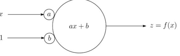
[image:3.595.231.523.617.708.2]

and consider a simple neuron model in [7] (see Figure 2)

(4)

DOI: 10.4236/apm.2018.85027 488 Advances in Pure Mathematics Here we use the linear function (1) instead of the sigmoid function z=σ

( )

x _.

In this case the square error function becomes

( )

(

( )

)

2

{

(

)

}

2

1 1

, .

2 2

n n

i i i i

i i

L a b y f x y ax b

= =

=

∑

− =

∑

− +

We usally use L a b

( )

, instead of E a b

( )

, in (2).

Our aim is also to determine the parameters

{ }

a b, in order to minimize

( )

,

L a b . However, the procedure is different from the least squares method in Section 1. This is an important and interesting point.

For later use let us perform a little calculation

( )

(

)

(

( )

)

( )

(

)

(

( )

)

1 1 1 1 , . n n

i i i i i

i i

n n

i i i i

i i

L _y _{f x} f _y _{f x x}

a a

L _y _{f x} f _y _{f x}

b b = = = = ∂ ∂ = − − = − − ∂ ∂ ∂ ∂ = − − = − − ∂ ∂

∑

(9)

We determine the parameters

{ }

a b, successively by the gradient descent method, see for example [8]. For t=0,1, , , n

( )

00

( )

(

11

)

a a t a t

b b t b t

     +  → → → →      ₊          and

(

)

( )

_{( )}

(

) ( )

_{( )}

1 , 1 , L

a t a t

a t L

b t b t

b t ∂ + = − ∂ ∂ + = − ∂   (10) where

( ) ( )

(

)

{

(

( )

)

}

2 1 1 , 2 n i i i

L L a t b t y a t x b t

=

= =

∑

− +

and _

(

0< <_ 1

)

_{is small enough. The initial value}

(

a

( ) ( )

0 , 0b

)

T is given appropriately. As will be shown shortly in Theorem I, their explicit values are not important.

Comment The parameter  is called the learning rate and it is very hard to choose  properly as emphasized in [7]. In this paper we provide an estimation (see Theorem II).

Let us write down (10) explicitly:

(

)

( )

{

(

( )

)

}

( )

1

2

1 1 1

1

n

i i i

i

n n n

i i i i

i i i

a t a t y a t x b t x

x a t x b t x y

= = = = + = + − +     = −_ _ − _ _ +    

∑

    and

(

) ( )

{

(

( )

)

}

( ) (

) ( )

1 1 1 1 1 . n i i i n n i i i i

b t b t y a t x b t

x a t n b t y

(5)

DOI: 10.4236/apm.2018.85027 489 Advances in Pure Mathematics These are cast in a vector-matrix form

(

)

(

)

(

)

( )

(

)

( )

(

)

( ) (

) ( )

( )

2

1 1 1

1 1

2

1 1 1

1 1 2 1 1 1 1 1 1 ₁ 1 1 1 0 0 1

n n n

i i i i

i i i

n n

i i

n n n

i i i i

i i i

n n i i i i n n i i i i n i

x a t x b t x y

a t

b t _{x a t} _{n b t} _y

x x a t x y

b t

x n y

x x x = = = = = = = = = = = = =  ₋ ₋ ₊   _{+  } _ =  ₊ _{ } _    − + − +     ₋ ₋ _ _       =_ _ +_ _ − −         = _ _−  

∑

           



( )

_{( )}

1

1 . n i i i n

i _i i

x y a t b t n y = =   _ _    _ _ ₊ _ _    _ _ _ _    _ _ _ _  

∑

 (11)

For simplicity by setting

( )

_{( )}

1 2 1 1

1 1

, ,

n n n

i i i i

i i i

n n

i i

x x x y

a t

t A

b t _x _n _y

= = = = =       _ _ _ _ =  =_ _ =_ _   _ _ _ _

∑

x f

we have a simple equation

(

t+ =1

) (

E A−

) ( )

t +

x  x f (12)

where E is a unit matrix. Due to (8) the matrix A is invertible (_∃_A−1_{), that is, we} exclude the trivial and uninteresting case x x1= 2==xn.

The solution is easy and given by

( ) (

_t ₌ _E₋ _A

) ( )

t ₀ ₊

{

_E₋

(

_E₋ _{A A}

)

t

}

−1 _.

x  x  f (13)

Note Let us consider a simple difference equation

(

1

)

( )

(

1

)

x n+ =ax n b+ a≠ for n=0,1,2,__{. Then, the solution is given by}

( )

0 1

( )

0 1 .

1 1

n n

n a n a

x n a x b a x b

a a

− −

= + = +

− −

Check this.

Comment The solution (13) gives

( )

1

lim

t t A

−

→∞x = f (14)

if

(

)

lim t

t→∞ E−A =O (15)

where O is a zero matrix. (14) is just the equation (5).

Let us evaluate (13) further. For the purpose we make some preparations from Linear Algebra [9]. For simplicity we set

2

1 1 1

1 1

,

n n n

i i i i

i i i

n n

i i

x x x y _e

A

f

x n y

α β

β δ

= = = = =   _ _   _{ }     =_ _≡_ _ =_ _≡_{ }        

∑

f

∑

and want to diagonalize A.

(6)

DOI: 10.4236/apm.2018.85027 490 Advances in Pure Mathematics

( )

(

)(

)

(

)

2

2 2

f λ λE A λ α β λ α λ δ β

β λ δ

λ α δ λ αδ β

− −

= − = = − − −

− −

= − + + −

and the solutions are given by

(

)

2 ₄

(

2

)

₍

₎

2 ₄ 2

.

2 2

α δ α δ αδ β α δ α δ β

λ_±= + ± + − − = + ± − + ₍₁₆₎

It is easy to see

0,

λ

+>

λ

−>

(

)

1 n andn 2 .

λ

₊>

δ

= ≥ ₍₁₇₎

We set the two eigenvectors of matrix A, corresponding to

λ

+ and

λ

−, in a matrix form

.

Q λ+_β δ _λ β_α −

−

 

=  ₋ 

 



It is easy to see

(

_{λ δ}

)

2 _β2

(

_{λ α}

)

2 _β2 2

+− + = −− + ≡ Λ

from (16) and we also set

1 _.

Q λ+_β δ _{λ α}β −

−

 

=  ₋ 

Λ   (18)

Then it is easy to see

T T T 1_.

Q Q QQ₌ _{= ⇒}E Q ₌Q−

Namely, Q is an orthogonal matrix. Then the diagonalization of A becomes T

0 . 0

A Q λ+ _λ Q

−

  =  

  (19)

By substituting (19) into (13) and using

T

1 0

0 1

E A Q λ+ _λ Q

−

 

− _{= } _

−

 

 



we finally obtain

Theorem I A general solution to (12) is

( )

(

)

₍

₎

( )

(

)

(

)

T

1 0 0

0

0 1

1 1

0

. 1 1

0

t

a t a

Q Q

b t b

e

Q Q

f

λ

λ λ λ

λ λ +

−

+ +

− −

 ₋ 

   

 

=

  _ _  

−

  _ _  

 _{− −} 

 

 

 

+ _ _ _{ }

  − −

 

 



 



(20)

This is our main result.

(7)

DOI: 10.4236/apm.2018.85027 491 Advances in Pure Mathematics very important problem in Deep Learning. Let us remember

0 and 1

λ

+>

λ

−>

λ

+>

from (17). From (15) the equations

(

)

(

)

(

)

lim t lim 1 t lim 1 t 0

t→∞ E−A = ⇔O t→∞ −λ+ =t→∞ −λ− =

determine the range of . Noting

(

)

(

)

1 1 0 2 lim 1 n 0

n

x x _→∞ x

− < ⇔ < < ⇒ − =

we obtain

Theorem II The learning rate  must satisfy an inequality

2

0 λ 2 0 .

λ +

+

< < ⇔ < < (21)

From (21)  becomes very small when

λ

+ is large enough. It is easy to see that the second condition limt→∞

(

1−λ−

)

t =0 is automatically satisfied.

Under Theorem II we can recover (14)

( )

T 1

1 ₀

lim

1 0

t

a t e

O O A

b t f

λ

+ −

→∞

−

 

 

  _ _  

= =

  _ _  

 

  _ _

 

f

by (19).

Comment For example, if we choose  like

2 ₁

λ₊ < <

then we cannot recover (14), which shows a difference between Statistics and Deep Learning. Let us emphasize that the choice of the initial values

( ) ( )

{

a 0 , 0b

}

is irrelevant when the convergence condition (21) is satisfied. As a result, how to choose  properly in Deep Learning becomes a very important problem when the number of data is huge. As far as we know the result like Theorem II has not been obtained.

3. Problem

In this section we present the outline of a simple generalization of the results in Section 2. The actual calculation is left as a problem (exercise) to readers.

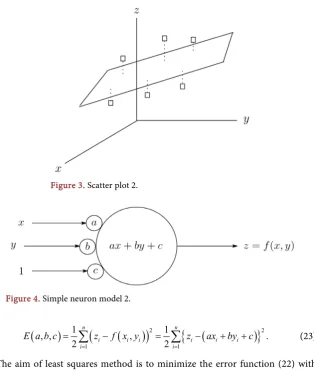
For n pieces of three dimensional real data

(

) (

)

(

)

{

x y z1, ,1 1 , x y z2, ,2 2 , , x y zn, ,n n

}

we assume that its scatter plot is like Figure 3

Then a model function is linear

( )

,

(8)

[image:8.595.221.536.66.438.2]

DOI: 10.4236/apm.2018.85027 492 Advances in Pure Mathematics Figure 3. Scatter plot 2.

Figure 4. Simple neuron model 2.

(

)

(

)

2

{

(

)

}

2

1 1

, , , .

2 2

n n

i i i i i i

i i

E a b c z f x y z ax by c

= =

=

∑

− =

∑

− + + (23)

The aim of least squares method is to minimize the error function (22) with respect to

{

a b c, ,

}

.

As we want to treat the least squares method above from the view point of Deep Learning, we again arrange the data like

(

) (

)

(

)

{

1 1 2 2

}

Input data : x y, ,1 , x y, ,1 , , x yn, ,1n

{

1 2

}

Teacher signal : , , ,z z  zn

and consider another simple neuron model (see Figure 4) Then we present

Problem Carry out the corresponding calculation as given in Section 2.

4. Concluding Remarks

In this paper we discussed the least squares method from the view point of Deep Learning and carried out calculation of the gradient descent thoroughly. A difference in methods between Statistics and Deep Learning delivers different results when the learning rate  is changed. The result of Theorem II is the first one as far as we know.

(9)

DOI: 10.4236/apm.2018.85027 493 Advances in Pure Mathematics from Mathematics. However we don’t know a good and compact textbook leading to Deep Learning.

I am planning to write a comprehensive textbook in the near future [10].

Acknowledgements

We wish to thank Ryu Sasaki for useful suggestions and comments.

References

[1] Wikipedia: Least Squares. https://en.wikipedia.org/wiki/Least_squares [2] Wikipedi: Deep Learning. https://en.wikipedia.org/wiki/Deep_learning

[3] Goodfellow, I., Bengio, Y. and Courville, A. (2016) Deep Learning. The MIT Press, Cambridge.

[4] Patterson, J. and Gibson, A. (2017) Deep Learning: A Practitioner’s Approach. O’Reilly Media, Inc., Sebastopol.

[5] Okaya, T. (2015) Deep Learning (In Japanese). Kodansha Ltd., Tokyo.

[6] Amari, S. (2016) Brain⋅Heart⋅Artificial Intelligence (In Japanese). Kodansha Ltd., Blue Backs B-1968, Tokyo.

[7] Fujii, K. (2018) Mathematical Reinforcement to the Minibatch of Deep Learning.

Advances in Pure Mathematics, 8, 307-320. https://doi.org/10.4236/apm.2018.83016

[8] Wikipedia: Gradient Descent. https://en.wikipedia.org/wiki/Gradient_descent [9] Kasahara, K. (2000) Linear Algebra (In Japanese). Saiensu Ltd., Tokyo.

[10] Fujii, K. Introduction to Mathematics for Understanding Deep Learning. In