Simulink/MATLAB Model for Assessing the Use of a Centrifugal Pump as a Hydraulic Turbine

(1)

ISSN Print: 2160-049X

DOI: 10.4236/wjm.2018.87021 Jul. 26, 2018 253 World Journal of Mechanics

Simulink/MATLAB Model for Assessing the Use

of a Centrifugal Pump as a Hydraulic Turbine

Peter E. Jenkins

*

, Artem Kuryachy

Mechanical Engineering Department, University of Colorado, Denver, USA

Abstract

A centrifugal pump used as a hydraulic turbine in producing power for a mi-crohydropower system is multifaceted. Centrifugal pumps are far more ubi-quitous than turbines in the turbomachinery market, therefore being more readily available to the consumer. Additionally, they are cheaper. Hydraulic turbines undergo rigorous CFD simulation design and testing to establish their blade geometries and ranges of operation. This results in a refined but very expensive final product. Centrifugal pumps are thus presented as a logi-cal alternative seeing that they can physilogi-cally perform the same task as a hy-dropower turbine albeit at a reduced efficiency. This paper presents the re-sults of an analysis and simulation to assess the use of a centrifugal pump as a hydraulic turbine.

Keywords

Centrifugal Pump, Hydraulic Turbine, Simulink, MATLAB Simulation

1. Introduction

Given the right hydrologic circumstances, a viable source of renewable energy can be found in hydropower. Hydropower is attained through the transfer of potential and kinetic energies stored in liquid into mechanical energy. This transfer is traditionally facilitated by a specific type of turbomachinery called a hydraulic turbine. However, this does not necessarily always have to be the case. For a microhydropower installation, there may be the option for this energy transfer to be performed by a centrifugal pump instead.

The reasoning for a centrifugal pump to be used instead of a hydraulic turbine in producing power for a microhydropower system is multifaceted. Centrifugal pumps are far more ubiquitous than turbines in the turbomachinery market, therefore being more readily available to the consumer. Additionally, they are

How to cite this paper: Jenkins, P.E. and Kuryachy, A. (2018) Simulink/MATLAB Model for Assessing the Use of a Centrifug-al Pump as a Hydraulic Turbine. World Journal of Mechanics, 8, 253-271.

https://doi.org/10.4236/wjm.2018.87021

Received: June 26, 2018 Accepted: July 23, 2018 Published: July 26, 2018

(2)

DOI: 10.4236/wjm.2018.87021 254 World Journal of Mechanics

cheaper. Hydraulic turbines undergo rigorous CFD simulation design and test-ing to establish their blade geometries and ranges of operation. This results in a refined but very expensive final product. Centrifugal pumps are thus presented as a logical alternative seeing that they can physically perform the same task as a hydraulic turbine albeit at a reduced efficiency [1].

Knowing this, it is worth investigating the viability of using a centrifugal pump in a microhydropower application for cost reduction. Is such a cost re-duction warranted in the context of reduced efficiency?

The Simulink/MATLAB simulation described within this work strives to aid in answering such a question. It uses the concept of flow geometry to describe the behavior of the three characteristic turbomachinery parameters (head, pow-er, efficiency) for two common types of centrifugal pump geometries (radial and backswept).

2. Simulink Model

The Simulink model is meant to allow for a readily available comparison be-tween pump and turbine modes for a turbomachine whose original purpose is that of a centrifugal pump. It is composed of four subsystems representing dif-ferent impeller operating modes and impeller geometries, as shown in Figure 1.

They include a backswept pump, backswept PAT, radial pump and radial PAT. Backswept impellers on a centrifugal pump have blades that sweep coun-terclockwise as they protrude from the center of the impeller. Conversely, radial impellers have blades that remain straight as they protrude outwards from the inner diameter to the outer diameter. All four employ the same constant values for gravity, density, inner diameter, outer diameter, and rotations per minute (RPM).

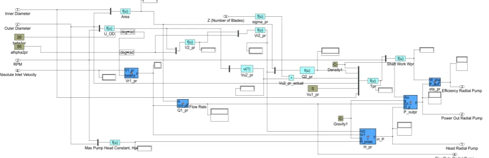
Figure 2 offers a more in-depth look into the radial pump subsystem. This subsystem, as do the rest, reads from left to right. This means that it receives in-puts on the left-hand side, called sources in Simulink, and then has outin-puts, also called sinks, finishing on the right.

(3)

[image:3.595.60.539.67.391.2]

[image:3.595.61.542.440.596.2]

Figure 1. Simulink model of two turbomachines, one radial and one of backswept geometry, for pump and pump-as-turbine modes.

Figure 2. Radial pump subsystem.

the user to write a mini-script. Seeing as the Simulink User-Defined Function blocks only allowed for scalar inputs, these MATLAB Function blocks were a must for dealing with the calculations that employed the inlet absolute velocity vector.

(4)

[image:4.595.58.539.121.506.2]

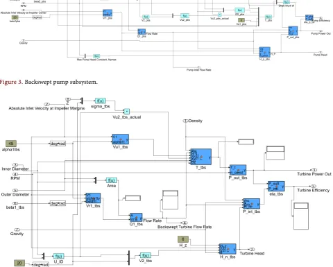
Figure 3. Backswept pump subsystem.

Figure 4. Backswept turbine subsystem.

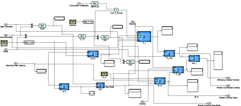
block and a mux block coming before. The purpose of the display block as the name implies is to show values in the simulation, without any additional prompting. Mux blocks serve to combine several different input signals to then output them as a vector or a bus output signal. This makes them convenient for use in combination with Simulink user-defined functions, seeing as one can effi-ciently track multiple scalar inputs inside a one-row vector.

(5)

[image:5.595.64.538.70.278.2]

Figure 5. Radial turbine subsystem.

Ultimately, the computations performed within these subsystems solve for multiple unknowns which eventually allow for the calculation of that turboma-chine’s head, power output and efficiency over a flow rate domain. The time step is set to zero so that the entirety of the inlet velocity vectors is taken instantly for the calculation. Seeing as the inlet velocity vector is the independent variable that drives the model and not time-dependent, this time step setting is necessary.

3. Flow Model

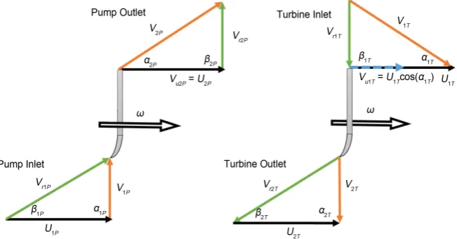
The flow model utilizes the concept of velocity triangles to solve for circumfe-rential, relative and whirl velocities along with flow rates for both inlet and out-let sections [2]. Velocity triangles describe the velocities of the fluid and turbo-machine at various points at both the inlet and the outlet. In total, there are eight triangles programmed into this Simulink model. There are two for backswept pump inlet and outlet, two for backswept PAT inlet and outlet, and the same ar-rangement for the radial geometry.

Circumferential velocity U as the name implies deals with the velocity at the circumferences of the inner and outer diameters. For backswept and radial cen-trifugal pumps, the inner and outer circumferential velocities are unequal. Rela-tive velocities Vr deal with the velocity of the fluid relative to that of the

rotat-ing blade. The whirl velocity Vu or Vw is the tangential (horizontal)

compo-nent to absolute velocity. Flow velocity Vf may also be present but is not

ne-cessary in the calculations done by this simulation. Absolute velocity V is fluid velocity that is relative to absolute space. The model calls for the use of two ab-solute inlet velocity vectors with one being used for the pump and one being used for a turbine. This is because the turbine mode sometimes requires a higher relative inlet velocity in order to achieve the same flowrates as the pump mode.

(6)

turboma-DOI: 10.4236/wjm.2018.87021 258 World Journal of Mechanics

chines as seen in Figures 6-8. The proportions of the triangles are characterized by their angles.

α

is the angle made by the absolute velocity with the circum-ferential velocity. β_{is the blade angle. The setting of}β_{to be less than 90˚}

creates a backswept blade geometry while β=90_{creates a radial geometry.} Geometric relationships become evident among αp and βp and their turbine

counterparts once a single centrifugal turbomachine is used for both pump and PAT operation modes.

While the relationship of 180−β2p =β1T is straightforward, that is not so

much the case for α1T. This angle would be needed to calculate the relative

tur-bine inlet velocity Vr₁_T if one were to use the Law of Sines. Instead, it is possible

[image:6.595.213.529.264.472.2]

to employ The Law of Cosines as seen in Equation (1) to try and circumvent the use of α1T.

Figure 6. Backswept pump outlet and backswept turbine inlet velocity triangles. The orange lines indicate the absolute velocity, the green lines represent the relative velocity, and the blue stand for the whirl velocity and the black line denotes circumferential velocity.

[image:6.595.211.537.534.704.2]

(7)

[image:7.595.210.540.70.284.2]

Figure 8. Graph of Equation (1) given angle values used in Table 2.

( )

1 2 2 1 2 1

1 2 cos

T T OD r OD T V U V U β − =

− ∗ ∗ (1)

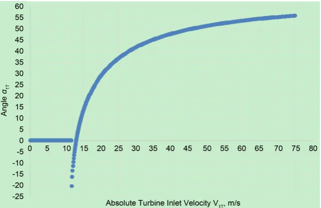
However, one can see that the resultant equation will not yield a real answer unless the absolute inlet turbine velocity exceeds the outer diameter circumfe-rential velocity. This is a constraint of this simulation because the rotations per minute is kept constant, therefore making the circumferential velocities constant as well. As such, it is not mathematically possible to compute α1T nor Vr1T, at

least before the desired RPM constant is reached. A low absolute inlet velocity cannot physically induce an instantaneous 500 RPM on the turbomachine. It becomes readily evident that in order to calculate α1tbs in relation to

2 1

180−β pbs=βtbs, the relative velocity Vr1T of the water entering the PAT has to

be larger than the PAT’s circumferential velocity UOD in order for the Turbine

Inlet triangle to be possible. Given an RPM of 500, the absolute inlet turbine ve-locity V1T would have be larger than 13.1 m/s before the relationship in

Equa-tion (1) would yield a real, non zero, result. After this point, the value of Vr₁_T

would follow the curve given in Figure 8 assuming that β2P=65 and knowing

that β1T =180−β2P =115. Therefore, an appropriate angle is assigned for the

sake of simulation which could also be measured if given an actual centrifugal pump.

3.1 Slip Factor

Slip factor is accounted for using the empirical correlations of Stanitz Equation (2) and Wiesner Equation (3).

( )

2

1.98 1

1 r cot

(8)

( )

2 0.7

sin 1

z

β

σ

= − (3)

It is defined as a measure of the deviation in angle at which the fluid leaves the impeller from the blade. This is represented as a ratio of the actual outlet whirl velocity divided by the ideal outlet whirl velocity, as seen in Equation (4).

actual ideal u u V V

σ= (4)

It accommodates slip loss in the calculation, a phenomenon that results due to a difference in pressure between the leading and following parts of the impeller blade. The addition of slip factor helps to create a noticeable increase in back-swept efficiency, seeing as it helps to illustrate the tendency of the fluid to “hug” the following side of the backswept blade during operation. This holds true only for the pump mode however, seeing as the outlet whirl velocity for a turbine is assumed to be zero.

4. Simulation Model

This model is driven by absolute inlet velocities that must be assigned and in-cremented as a one-dimensional vector inputs. They begin at zero and incre-ment at intervals of 0.1 m/s up to the maximum assigned absolute inlet velocity, with each interval yielding new values for head, power and efficiency at the spe-cified mode.

The No-Slip condition was applied on the inlets for the pump mode and the outlets for the Pump-As-Turbine mode. This resulted in the whirl velocities Vu

in these areas being declared zero. This is due to the structure of the velocity triangle, which in those locations is a right triangle that therefore eliminates the whirl velocity Vu and the slip phenomenon. System curves were not generated

due to a lack of pressure data for the suction and discharge regions. Losses were also declared negligible. The starting angle values for the velocity triangles were assumed as well based on typical centrifugal pump geometries. Only the smallest possible number of angles was declared, and the rest were attempted to be solved for based off the impeller geometries. The typical constants for gravity and water density were used.

4.1. Accompanying MATLAB Code

(9)

inlet absolute velocity. Any value that does not require existing as a vector exists as a scalar quantity, thereby explaining the lack of vectors in the outlet sections of the loops. The equations used in the calculation portion of this script are identical to those used in the Simulink model. Upon termination of the loops, MATLAB’s graphing functions are employed to generate the twelve final plots.

4.2. Discussion of Equations Used

All computations and results are presented in SI units. As such, some conversion factors are present within the model and code equations. This is evident with one of the first computations, the Shut-off head, also known as maximum pump head. It was calculated using Equation (5), which was in customary units thereby requiring the conversion of the outer diameter into feet and then the conversion of the head result back into meters.

(

_39.3701

)

2 2

1750 3.280 so OD p n d H ∗ ∗_ _  

= (5)

The circumferential velocities of Equation (6) and Equation (7) are computed as a product of the RPM and the respective diameter, with a linearizing conver-sion factor to address the rotation.

π

60

ID

ID d

U = n ₍₆₎

π

60

OD

OD d

U = n ₍₇₎

Seeing as the model computes using a constant RPM, this thereby makes the circumferential velocity constant as well. As mentioned previously, the other ve-locities are computed using triangular relationships such as the law of sines, co-sines and right triangle rules.

The Pump Head equation used is Equation (8).

2 2 2 1 2 so r r p p V V H H g −

= + ₍₈₎

It is a summation of the shut-off head along with the difference between the squared outlet and inlet relative pump velocities. Pump head can be defined as the amount of pressure that a pump can supply to the fluid. It is then used in Equation 6 to compute the power out, the power transferred from the pump to the fluid via mechanical energy.

Similarly, turbine head in Equation (9) is a summation of the difference be-tween the squared inlet and outlet turbine relative velocities plus the static head that the turbine is operating at.

2 2

1 2

2

nt z V V

H H

g

−

= + ₍₉₎

(10)

through Equation (10) and Equation (11).

2 2 actual ₂ 1 ₂

OD ID

pbs pbs u pbs u pbs

d d

T =

ρ

Q _V _ _−V _ __

 

  (10)

2π

60

pbs

shaft pbs

W =T n ₍₁₁₎

The torque equation itself is a form of Euler’s Turbomachinery Equation. It is the difference in the fluid through the turbomachine. For the Pump-As-Turbine mode, the outlet whirl velocity Vu2t was assumed to be zero, thereby making

the power dependent solely on the inlet velocities as seen in Equation (12) and Equation (13).

1 1t ₂

OD t t u

d T =

ρ

Q V _ _

  (12)

2π

60

t

out t

P =T n ₍₁₃₎

The turbine efficiency of Equation (14) is instead a ratio for power output, the power produced by the turbine also turbine shaft work, to power input, which is the hydraulic power of the water entering the system.

tbs tbs out tbs in P P

η = (14)

5. Discussion of Results

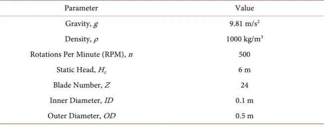
The simulation model was run using the parameters listed in Table 1 and the angles listed in Table 2.

The results are twelve graphs presented in Figures 9-20. Graphs of Figures 9-14 compare parameters between pump and turbine modes for their respective geometries, while the graphs of Figures 15-20 compare parameters between geometries for their respective modes.

Figure 9 is a comparison of the turbine head to the pump head for a back-swept impeller geometry.

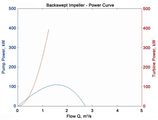
[image:10.595.272.531.88.152.2]

Under the given conditions, the backswept pump mode is unable to provide any more head to the fluid once flow rate exceeds 2.6 m3_{/s. This is why the power}

Table 1. Selected constants.

Parameter Value

Gravity, g 9.81 m/s2

Density, ρ 1000 kg/m3

Rotations Per Minute (RPM), n 500

Static Head, Hz 6 m

Blade Number, Z 24

Inner Diameter, ID 0.1 m

[image:10.595.209.537.599.734.2]

(11)

[image:11.595.207.536.100.608.2]

Table 2. Selected angle values. The angles whose value includes another angle indicate a geometric relationship.

Angle Value

1pbs

α 90˚

1pbs

β _20˚

2pbs

α 20˚

2pbs

β 65˚

2pbs

γ 180−α2pbs−β2pbs

1tbs

α 45˚

1tbs

β 180−β2pbs

2tbs

α α1pbs

2tbs

β β1pbs

1pr

α 90˚

1pr

β 20˚

2pr

α _45˚

2pr

β 90˚

1tr

α α2pr

1tr

β β2pr

2tr

α α1pr

2tr

[image:11.595.209.535.102.606.2]

β β1pr

Figure 9. Head curve-backswept impeller.

output for the backswept pump mode terminates at 2.6 m3_{/s, while the}

back-swept turbine mode power output continually increases with flow rate in Figure 10.

(12)

[image:12.595.222.525.67.298.2]

Figure 10. Power curve-backswept impeller.

Figure 11. Efficiency curves.

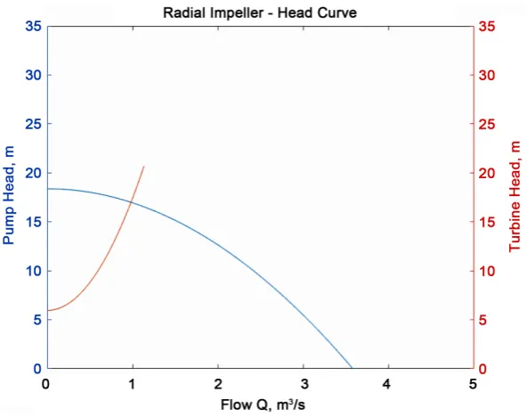
The radial impeller geometry head curve of Figure 12 shows the pump head beginning at approximately 17 m and terminating at 0 m when the flow rate reaches approximately 3.5 m3_/s.

The power curve for the radial pump mode shown in Figure 13 is much larger than its backswept counterpart in Figure 10.

[image:12.595.225.523.324.561.2]

(13)

[image:13.595.226.523.70.304.2]

[image:13.595.226.524.335.573.2]

Figure 12. Radial impeller-head curve.

Figure 13. Radial impeller-power curve.

velocity is much larger for the radial configuration under the given velocity tri-angle tri-angles. This explains why the radial pump power curve in Figure 13 is larger than its backswept counterpart in Figure 10.

An unexpected but explainable result is shown in Figure 14. The turbine mode is more efficient than the pump mode for the radial configuration by about 25%, but severely limited in it’s operational flow rate. It terminates at about 76% for 1 m3_{/s. This is due to the geometric variation for the intake of}

(14)

[image:14.595.223.526.68.301.2]

Figure 14. Radial impeller-efficiency curve.

Figure 15. Backswept and radial impellers in turbine mode.

for a radial impeller has the water coming in at a blade angle β<90_{while it’s} turbine counterpart has the water entering at β=90_{. This means that}

1TR 1PR

Q ≠Q , the inlet flow rates are not equal between pump and PAT mode. In fact, Q1TR<Q1PR along the entirety of the absolute inlet velocity vector. This

ex-plains why the pump mode is able to produce power over a larger flow rate do-main than the turbine. Additionally, the PAT efficiency of Equation (14) is de-pendent on the inlet flow rate through its denominator Pin_TR. The Equation (15)

[image:14.595.225.521.325.570.2]

(15)

[image:15.595.225.523.67.299.2]

[image:15.595.224.522.328.562.2]

Figure 16. Power curves for backswept and radial impellers in turbine mode.

Figure 17. Efficiency curves for backswept and radial impellers in pump mode.

thereby contributes to an overall smaller denominator for the efficiency calcula-tion of Equacalcula-tion (14) and therefore a higher turbine efficiency.

1

t

in t nt

P =ρgQ H ₍₁₅₎

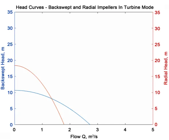
Figure 15 shows the turbine head for the radial and backswept geometries. The radial turbine head, as mentioned previously, starts off about 7 m higher than the backswept turbine head. Its slope however is more aggressive and it terminates earlier as a result.

(16)

[image:16.595.225.521.70.303.2]

Figure 18. Head curves for backswept and radial impellers in turbine mode.

Figure 19. Power curves for backswept and radial impellers in turbine mode.

The backswept efficiency is significantly larger in pump mode than the radial ef-ficiency, by approximately 30% as showcased in Figure 17.

The radial turbine mode provides essentially the same amount of head and thereby the same amount of power as the backswept turbine mode, while doing so more gradually over a longer flow rate domain. This can be seen in Figure 17 and Figure 18.

[image:16.595.223.525.337.571.2]

(17)

[image:17.595.224.526.72.300.2]

Figure 20. Efficiency curves for backswept and radial impellers in turbine mode.

shown in Figure 20.

6. Simulation Model Limitations

The fundamental limitation of this simulation model is that there is not yet a way to predict the outlet velocities so that they can change depending on inlet velocity. With the configuration of the model as it is now, the outlet velocities are constants that depend on the circumferential velocity, which in and of themselves are constant due to a constant RPM. To put it in terms of values, it is not physically feasible for an absolute inlet speed of 0.1 m/s to translate into an absolute outlet speed that is dependent on a circumferential velocity calculated using 500 RPM. This insinuates why changes in certain angle values or machine parameters can cause the efficiency to either become negative or larger than one. Ideally, Euler’s Equation for Turbomachinery would be used to find the outlet velocity while incrementing the inlet velocity. This would however require the manufacture to provide head curve data. Using this, the outlet velocity for a given head curve could be computed while varying the inlet velocity. This could then be used as a basis to calculate the remaining velocities.

The fact that the absolute outlet velocity cannot be computed in the model means that the constant circumferential velocity must be relied upon when try-ing to describe a geometric relationship between the backswept pump outlet and backswept turbine inlet angles. It becomes readily evident that in order to calcu-late α1tbs in relation to180−β2pbs=β1tbs, the relative velocity Vr1T of the water

entering the PAT has to be larger than the PAT’s circumferential velocity UOD

in order for the Turbine Inlet triangle to be possible. Figure 6 illustrates this vi-sually and Equation (1) describes this mathematically via Law of Cosines.

(18)

equivalent to the outer diameter circumferential velocity, unlike outlet whirl ve-locity for the radial pump. This is somewhat surprising seeing as the geometries of the two configurations are identical. It is not surprising though when ex-amined in the context of the constant RPM. The model assigns the turbine inlet a circumferential velocity based on 500 RPM for the entirety of the absolute inlet velocity vector, from 0.1 m/s to it’s maximum. This is not physically feasible.

Turbines typically do operate at constant RPM values, so the fact that the model is set to do so is not abnormal. This is because it is often desirable to maintain a balance between the Prime Mover Torque and the Electromagnetic Drag in the generator. If this is done, then the rotor speed will remain constant. The power generated in the turbine comes from the prime mover shearing it’s magnets against the magnetic field of the stator windings, thereby generating electromagnetic drag. The stator windings are copper structures which facilitate the transfer of the kinetic energy to electric energy.

7. Conclusions

Keeping in mind the limitations that this model possesses, it can still be used as a starting point for assessing the viability of the use of a centrifugal pump as a PAT machine. If head curves from a manufacturer can be acquired at a desired constant RPM, especially the equations for these curves, it can be easily adjusted to provide the correct results.

As it stands currently, it can be used to facilitate a simple comparison. It can give the user a potential gauge of the size, geometry and blade number. Addi-tionally, it is necessary to note that the values of Torque and Power Output for the Backswept and Radial Turbines are correct. This is due to the No-Slip condi-tion that assigned for both the pump inlet and the turbine outlet, in which it re-sulted in the Outlet Turbine Whirl Velocity Vu₂_t being 0.

The zero Whirl Velocity is a common assumption for turbines as it idealizes the complete transfer of energy from fluid to kinetic form. With this in mind, one can see that Equation (12) and Equation (14) all change in response to the change in the inlet velocity. The curves that they provide are quite reasonable as well, as seen in Figure 20 above.

Given the head curves at a specified RPM, after some adjustments, the model can be used to create a value index. This index would be a ratio of turbomachine cost to its efficiency. This way, a centrifugal pump operating as a PAT could be then compared to a turbine in terms of dollars per percent of efficiency. The higher the ratio is, potentially the worse the choice will be. A lower ratio would mean that the turbomachine would initially cost less but run more effectively. Such may be expected for a centrifugal pump seeing as they are significantly lower in price than microhydropower turbines.

References

[1] Dixon, S.L. (1998) Fluid Mechanics and Thermdynamics of Turbomachinery. El-sevier Publication, Amsterdam.
[2] Engineering ToolBox (2010) Centrifugal Pumps and Shut-Off Head.