Evolutionary Computation for Static Traffic Light Cycle Optimisation

Evolutionary Computation for Static

Traffic Light Cycle Optimisation

Eltayeb K. E. Ahmed

, Amr M. A. Khalifa

, Ahmed Kheiri

Department of Electrical and Electronic Engineering Algamaa Street, P.O. Box 321, Khartoum, Sudan

{eltayeb.k.ahmed, amr.khalifa.m.a}@gmail.com †_{Lancaster University, Department of Management Science}

Lancaster University Management School Lancaster, LA1 4YX, United Kingdom

[email protected]

Abstract—Cities have become congested with traffic and changes to road network infrastructure are usually not possible. Thus, researchers and practitioners are investigating the practice of traffic light signal optimisation methodologies upon already established road networks to improve the flow of vehicles through the cities. The flow of traffic can be described by multiple factors such as mean journey time, mean waiting time, average vehicle velocity, and time loss. Static timing means that each traffic phase is active for a pre-fixed duration during the cycle. We aim to optimise traffic signal timing plans to minimise the

mean journey time, which is increased by improper signalling, for vehicles during their journey across the junctions. In this research, we propose and empirically analyse several automatic intelligent decision support systems including genetic algorithms and selection hyper-heuristic methods for the optimisation of traffic light signalling problem. The empirical results indicate the success of the proposed algorithm techniques.

Index Terms—Transportation, Traffic Optimisation, Genetic Algorithms, Hyper-heuristics

I. INTRODUCTION

There have been a growing number of studies concerning the optimisation of traffic light signalling because it offers a way to increase the throughput of roads with no additional cost. The problem can be broadly grouped under the following main categories; static traffic lightsandadaptive traffic lights [1]. The former class operates on fixed timings, and the latter reacts to the current state of the road via sensors. This study focuses on optimising static traffic lights.

The traffic light cycle optimisation problem is considered a highly complexN P-hard optimisation problem, for which ex-act methods (such as mixed integer programming techniques) are unsuitable. There is a wide and varied literature on the use of novel heuristic methods for the optimisation of traffic light signalling [2]. These methods have proven to be very effective at finding near-optimal solutions to a large number of problems in the transportation field.

A relatively new breed of optimisation algorithms known as hyper-heuristics are beginning to be applied to these problems. Hyper-heuristics are automated methodologies for selecting or generating heuristics to solve multiple computationally difficult optimisation problems [3]. They combine several

fairly simple low level heuristics to create bespoke approaches for a given optimisation problem domain. Both types of hyper-heuristics (selection or generation) have proven successful on many difficult optimisation problems (see for example [4], [5]). To the best of the authors’ knowledge, the use of hyper-heuristics for this problem domain remains unexplored in the scientific literature.

This work investigates the use of genetic algorithms and selection hyper-heuristics to static traffic light cycle optimi-sation problem that could outperform conventional manual approaches in terms of solution quality.

The structure of this paper is as follows. Section II describes the problem dealt with in this work and discusses previous work. Section III describes the developed methods including the algorithmic components, operators and low level heuristics. The computational experiments and empirical results are pre-sented in Section IV. Finally, in Section V we discuss overall conclusions and future work.

II. BACKGROUND

A. Traffic Light Cycle Optimisation Problem

Traffic light timing cycles problem is a well-known real-world optimisation problem. A solution for the problem re-quires tuning the timing of each traffic light cycle in the network. Optimisation methods generally aim to minimise travel time of vehicles, and maximise the total traffic flow at a given intersection. A solution is simulated by a traffic simulator which provides the information necessary to evaluate the candidate solution under optimisation.

considering overall delays in the network. In addition to genetic algorithms, other heuristics have been successfully applied to this problem. Burvall and Oleg˚ard [9] applied simu-lated annealing to optimise traffic flow in a single intersection network. They reported that simulated annealing scales better than genetic algorithm for the parametrisations used. They argued that simulated annealing applications tend to be limited to small instances and population-based approaches such as genetic algorithms are more suited to larger instances.

B. Heuristic Methods

Heuristic optimisation algorithms guide the computational search required for finding solutions to problems, typically

N P-hard problems, where the optimal solutions cannot be found due to time and computing power constraints.

1) Genetic algorithm: Genetic algorithm (GA) was in-troduced by John Holland in the mid 70’s [10]. GA is a population-based heuristic technique inspired by Charles Darwins theory of natural evolution and it belongs to the class of evolutionary computation algorithms. In GA, a chromosome is a set of variables, referred to as genes, which defines a solution to the tackled optimisation problem [11]. A pool of solutions for a given optimisation problem is evolved through an evolutionary cycle, also known aspopulation generation, to obtain an efficient near-optimal solution at the end. The main components of genetic algorithms are selection, crossover, mu-tation and replacement. Firstly, parent individuals areselected from the pool of solutions. The selection can be simple random meaning that chromosomes are selected at random, or the selection can favour the high quality solutions (fitness propor-tionate selection). Other selection methods include: roulette wheel selection, ranked selection and tournament selection. Selected solutions are then recombined using a crossover operator, generating new solutions which are then subjected to mutation perturbing those new individuals further. Many crossover techniques exist. One-point crossover is the most popular crossover at which a random point is selected between [0, l−1], where l is the length of the chromosome. All data beyond that point are exchanged to form new offsprings. Mutation operators are used to maintain the diversity of solutions and researchers argue that mutation is useful to allow the algorithm to escape local minima. In this operation, a gene (or group of genes) in the chromosome is altered by randomly changing the gene’s value, swapping two genes, or randomly shuffling a subset of the genes. Finally, the replacement (reinsertion) component decides which solutions will survive to the next generation. A simple genetic algorithm is outlined in Algorithm 1.

2) Hyper-heuristic: Hyper-heuristic research has been growing since the initial ideas emerged in 1960s [12]. The term hyper-heuristic was initially defined in the early 2000s as a ‘heuristics to choose heuristics’ [13]. A number of review papers on hyper-heuristics have been published. The earliest appeared in [14], where the authors introduced the idea of hyper-heuristics and emphasised one of the key aims, namely, to raise the level of generality at which optimisation systems

Algorithm 1: Genetic algorithm

1 letf(x)be the objective we seek to minimise 2 population←initialise();

3 repeat

4 parents←select(population, 2); 5 of f spring←crossover(parents); 6 of f spring←mutation(of f spring);

7 worstChromosome←getWorstSolution(population) 8 iff(of f spring)< f(worstChromosome)then

9 population.pop(worstChromosome);

10 population.insert(of f spring); 11 end

12 untiltermination criterion is satisfied; 13 returngetBestSolution(population);

can operate. A more recent overview and tutorial chapter [15] discussed a class of hyper-heuristic that generates heuristics from a set of heuristic components. Burke et al. [16] provided a unified classification of hyper-heuristics that captures the work that was being undertaken at the time in the field of hyper-heuristics.

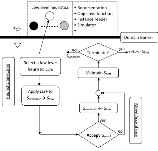
There are two main components in a single-point-based search selection hyper-heuristic:heuristic selectionthat selects a low level heuristic and applies it to the candidate solution, and move acceptance which decides whether to accept or reject the newly generated solution. The existence of a logical interface (as illustrated in Figure 1) between the selection hyper-heuristic and problem domain, referred to as domain barrier, prevents the hyper-heuristic to retrieve any problem-specific information and increases the level of generality and the reusability of the selection hyper-heuristic components, which can then be used across different problem domains without any modification.

The simplest form of a selection hyper-heuristic is a method that combines a simple random heuristic selection method (SR) with an improve or equal acceptance method (IE). Simulated annealing (SA) [17] has been applied as a move acceptance method in selection hyper-heuristics by several studies (see for example [18]). In SA, the probability of accepting worsening moves is given by the formula:

p=e−∆Tf (1)

Apply LLHito Scandidate →Snew

Accept Snew?

return Sbest

yes

no no

Sinitial

H

e

u

ri

st

ic

S

e

le

ct

io

n

M

o

v

e

A

cc

e

p

ta

n

ce

Scandidate Snew

Terminate?

Maintain Sbest Scandidate

yes

Domain Barrier

Select a low level heuristic LLHi

Low level heuristics • Representation • Objective function • Instance reader • Simulator • . . .

Fig. 1. A selection hyper-heuristic framework

Algorithm 2: Selection hyper-heuristic algorithm

1 Let LLH represent the set of low level heuristics 2 Let Scandidaterepresent the current solution 3 Let Sbest represent the best solution 4 Sinitial← initialise();

5 Sbest←Sinitial;

6 Scandidate←Sinitial;

7 repeat

8 LLH_i←Select(LLH);

9 S_new← ApplyHeuristic(LLH_i, S_candidate); 10 Sbest←updateBestSolution(Snew);

11 if Accept(Scandidate, Snew)then 12 Scandidate←Snew;

13 end

14 until termination criterion is satisfied; 15 return Sbest;

III. METHODOLOGY

Simulation of traffic light control on a single intersection is used as our case study. The traffic is controlled by an eight phase traffic light. Each phase represents a different state of the traffic light. In this study, all the phases are set with a fixed amount of time (3 seconds) except the phases

{0, 4} which correspond to the time that the green light phase is active in the directions North-South, and East-West, respectively. This study aims to optimise the flow of traffic by tuning the amount of time the traffic light spends in the{0, 4}

phases. The proposed heuristic approaches described in Sec-tion II-B (genetic algorithm GA, simple random with improve or equal move acceptance hyper-heuristic SR-IE, and simple random with simulated annealing move acceptance

hyper-Fig. 2. The problem scenario

heuristic SR-SA) are implemented in this study using an open source microscopic inter- and multi-modal space-continuous and time-discrete traffic flow simulation platform, referred to as SUMO “Simulation ofUrbanMObility” [19], designed for benchmarking purposes and it encapsulates problem domain specific details. We used thenetedittool andrandomT rips.py script within SUMO to design the intersection and generate the traffic for our case study problem (see Figure 2).

The traffic consists of 528 vehicles departing at times between 0s and 800s. The simulation is run until the last vehicle exited the traffic network or a time limit of 3000s is exceeded. The latter condition occurs when very poor timing configurations were tested. Several metrics were used to evaluate the quality of timing configurations, including: mean vehicle journey time (s), mean vehicle speed (m/s), mean vehicle waiting time (s) (defined as the time a vehicle spends on the road during its journey with a speed of less than 0.1m/s) and mean time loss (s) (defined as the time lost due to driving below the ideal speed). We set the mean vehicle journey duration as the main objective function to minimise as it is the most tangible benefit to the users of the road.

A candidate solution is encoded by a 2-coordinate vector of type integer that contains the durations of two corresponding traffic light phases. Selection hyper-heuristics operate by using a prefixed pool of low level heuristics by which a randomly initialised solution is improved over the search time. Four low level heuristics that perturb a given solution in different ways are used under the problem domain implementation of the selection hyper-heuristic framework:

• LLH1: Increase or decrease a randomly selected compo-nent of the solution (i.e. the amount of time the traffic light spends in the randomly selected phase) by a random number between [0, 5]

• LLH2: Increase or decrease a randomly selected compo-nent of the solution by 10

• LLH3: Increase or decrease a random number of com-ponents by a random number between [0, 1]

• LLH4: Swap two components of the solution at random

TABLE I

PARAMETERS OF THE GENETIC ALGORITHM

Parameter Value

Population size 4

Crossover type one-point

Mutation rate 50%

Selection random selection

is initially set to 1 and multiplied by a cooling factorof 0.99 each iteration. These values are set after a small number of preliminary experiments. Table I provides the parameter values for GA.

IV. EMPIRICALRESULTS

The experiments were conducted on an i7-4500U CPU with a memory of 8GB RAM. The three algorithms were run for ten times and the termination criterion is set to 1000 function evaluations. Mann-Whitney-Wilcoxon test, with 95% confidence level, was performed to compare pairwise statistical variations of two given approaches. Given Ma versus Mb, (i) Ma > Mb denotes that Ma is better than Mb and this performance difference is statistically significant, (ii) Ma < Mb denotes that Mb is better than Ma and this performance difference is statistically significant, (iii) Ma ' Mb denotes that there is no statistical significant between the two methods. SUMO provides a default configuration as a baseline whose performance is compared to the proposed heuristic methods, SR-IE, SR-SA and GA. Our experiments evaluate the solutions from the mean journey time perspective.

Table II presents the results, which clearly shows that the proposed methods, SR-IE, SR-SA and GA, improve signifi-cantly on the performance of the SUMO default configuration. In both Table II and Table IV, the columnbestfor each metric criterion is defined as the value of the criterion of the solution that has the lowest objective value, not necessarily the best value achieved for that criterion. Based on the Mann-Whitney-Wilcoxon test with respect to the averages over 10 runs on the problem scenario (see Table III), there is statistically significant performance differences between GA and SR-IE. In overall, the genetic algorithm seems to perform the best, followed by Simple Random with Simulated Annealing (SR-SA) hyper-heuristic. However, this performance difference between GA and SR-SA is not statistically significant.

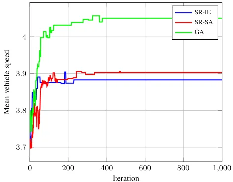
Figures 3-6 provide the average of changes in the mean journey time, mean vehicle speed, mean time loss and mean waiting time (all from mean journey time perspective) versus iteration from 10 runs while solving the problem scenario for 1000 iterations. It can be observed that the three approaches rapidly improve the quality of the best-of-run solution in hand. This improvement slows down over time. The fluctuations due to the simulated annealing move acceptance component in SR-SA and the employment of the perturbative operators (i.e. crossover and mutation) in GA help the search in SR-SA and GA to explore different search regions leading to an improved

0 200 400 600 800 1,000

140 145 150

Iteration

Mean

journe

y

time

SR-IE SR-SA GA

Fig. 3. Average of changes in the objective function value (the lower the better)

0 200 400 600 800 1,000

3.7 3.8 3.9 4

Iteration

Mean

v

ehicle

speed

SR-IE SR-SA GA

Fig. 4. Average of changes in the mean vehicle speed (from mean journey time perspective) (the higher the better)

solutions even if it takes some time to do so. It is clearly observed that while solving the problem scenario, the three algorithms seem to generate continuous improvements until they converged after about 400 iterations.

When optimising a certain parameter such as mean journey time, an optimisation algorithm will tend to prioritise traffic from the direction with the majority of the traffic, which in the case of heavily unbalanced traffic might lead to extremely long waiting times for those in the minority. To quantify this phenomenon, we introduced two new measures to evaluate the fairness of the flow, namely the VSSD (Vehicle Speed Stan-dard deviation) and JTSD (Journey Time StanStan-dard Deviation). These measures can provide an insight into how the fairness of the different traffic light controllers in the same problem scenario compare. A comparison between the algorithms using the two metrics is shown in Table IV.

TABLE II

SUMMARY OF EXPERIMENTAL RESULTS. BEST VALUES ARE HIGHLIGHTED IN BOLD

Mean Journey Time Mean Vehicle Speed Mean Time Loss Mean Vehicle Waiting Time

Algorithm Best Avg. Std. Best Avg. Std. Best Avg. Std. Best Avg. Std.

SUMO Default 163.41 - - 2.94 - - 134.60 - - 92.79 -

-SR-IE 137.98 141.52 2.57 3.83 3.88 0.15 109.17 112.71 2.57 75.36 79.73 2.40

SR-SA 138.13 140.36 1.81 3.87 3.90 0.16 109.31 111.54 1.81 77.41 78.94 1.26

GA 136.91 138.68 1.22 4.38 4.05 0.25 108.10 109.86 1.21 77.50 77.65 1.12

TABLE III

PAIRWISE PERFORMANCE COMPARISON OFSR-IE, SR-SAANDGA

SR-IE SR-SA GA

SR-IE – ' <

SR-SA ' – '

GA > ' –

0 200 400 600 800 1,000

110 115 120

Iteration

Mean

time

loss

SR-IE SR-SA GA

Fig. 5. Average of changes in the mean time loss (from mean journey time perspective) (the lower the better)

0 200 400 600 800 1,000

78 80 82 84 86 88

Iteration

Mean

w

aiting

time

SR-IE SR-SA GA

Fig. 6. Average of changes in the mean waiting time (from mean journey time perspective) (the lower the better)

TABLE IV

VSSD (VEHICLESPEEDSTANDARD DEVIATION)ANDJTSD (JOURNEY TIMESTANDARDDEVIATION). BEST VALUES ARE HIGHLIGHTED IN BOLD

VSSD JTSD

Algorithm Best Avg. Best Avg.

SUMO Default 2.09 - 81.04

-SR-IE 2.32 2.66 73.21 75.41

SR-SA 2.62 2.49 77.27 74.18

GA 3.20 2.80 84.50 76.69

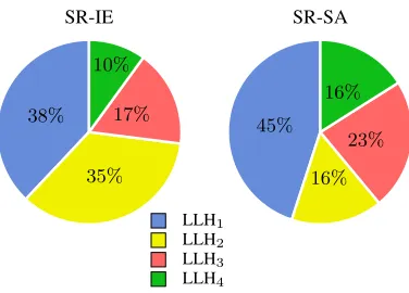
level heuristic over 10 runs in SR-IE and SR-SA considering the invocations that generated improvements on the best-of-run solution. It is noted that LLH1is the most successful low level heuristic in both algorithms, being responsible for the highest percentage of improvement on best-of-run solution.

SR-IE SR-SA

LLH1

LLH2

LLH3

LLH4 38%

35% 17% 10%

45%

16% 23% 16%

Fig. 7. Average utilisation rate

V. CONCLUSION

known to be computationally expensive because they require multiple calls of the simulator per iteration. In this study, we introduced two metrics to measure the fairness of traffic flow. No attempts were made to optimise with fairness as an objective. This research has potential to be implemented in many countries such as Sudan where traffic sensors are not widely deployed. The use of heuristic methods in this way will open doors towards a more collaborative environment where engineer and computer algorithm work together to solve such difficult problems without any costly new apparatus. The only information required by the proposed heuristic methods is the vehicle flow from each direction at peak hours, recorded to synthesise a realistic simulation of the scenario. The timing cycles of existing traffic lights could then be reconfigured to the near-optimal results obtained by these optimisation methods.

REFERENCES

[1] X. F. Xie, S. F. Smith, T. W. Chen, and G. J. Barlow, “Real-time traffic control for sustainable urban living,” in17th International IEEE Conference on Intelligent Transportation Systems (ITSC), Oct 2014, pp. 1863–1868.

[2] J. Garc´ıa-Nieto, A. C. Olivera, and E. Alba, “Optimal cycle program of traffic lights with particle swarm optimization,”IEEE Transactions on Evolutionary Computation, vol. 17, no. 6, pp. 823–839, 2013. [3] E. K. Burke, M. Gendreau, M. Hyde, G. Kendall, G. Ochoa, E. ¨Ozcan,

and R. Qu, “Hyper-heuristics: a survey of the state of the art,”Journal of the Operational Research Society, vol. 64, no. 12, pp. 1695–1724, Dec 2013.

[4] A. Kheiri and E. Keedwell, “A hidden markov model approach to the problem of heuristic selection in hyper-heuristics with a case study in high school timetabling problems,”Evolutionary Computation, vol. 25, no. 3, pp. 473–501, 2017.

[5] A. Kheiri and E. ¨Ozcan, “An iterated multi-stage selection hyper-heuristic,”European Journal of Operational Research, vol. 250, no. 1, pp. 77–90, 2016.

[6] M. E. Fouladvand, Z. Sadjadi, and M. R. Shaebani, “Optimized traffic flow at a single intersection: traffic responsive signalization,”Journal of Physics A: Mathematical and General, vol. 37, no. 3, p. 561, 2004. [7] N. M. Rouphail, B. B. Park, and J. Sacks, “Direct signal timing

optimization: Strategy development and results,” inIn XI Pan American Conference in Traffic and Transportation Engineering. Citeseer, 2000. [8] T. Kalganova, G. Russell, and A. Cumming, “Multiple traffic signal control using a genetic algorithm,” inArtificial Neural Nets and Genetic Algorithms. Springer, 1999, pp. 220–228.

[9] B. Burvall and J. Oleg˚ard, “A comparison of a genetic algorithm and simulated annealing applied to a traffic light control problem : A traffic intersection optimization problem,” 2015.

[10] J. Holland,Adaptation in Natural and Artificial Systems. Ann Arbor, MI, USA: University of Michigan Press, 1975.

[11] M. Mitchell,An Introduction to Genetic Algorithms. Cambridge, MA, USA: MIT Press, 1998.

[12] H. Fisher and G. L. Thompson, “Probabilistic learning combinations of local job-shop scheduling rules,” inIndustrial Scheduling, J. F. Muth and G. L. Thompson, Eds. New Jersey: Prentice-Hall, Inc, 1963, pp. 225–251.

[13] P. Cowling, G. Kendall, and E. Soubeiga, “A hyperheuristic approach to scheduling a sales summit,” inSelected papers from the Third Inter-national Conference on Practice and Theory of Automated Timetabling. London, UK: Springer-Verlag, 2001, pp. 176–190.

[14] E. K. Burke, E. Hart, G. Kendall, J. Newall, P. Ross, and S. Schulenburg, “Hyper-heuristics: An emerging direction in modern search technology,” inHandbook of Metaheuristics, F. Glover and G. Kochenberger, Eds. Kluwer, 2003, pp. 457–474.

[15] E. K. Burke, M. R. Hyde, G. Kendall, G. Ochoa, E. ¨Ozcan, and J. R. Woodward, “Exploring hyper-heuristic methodologies with genetic programming,” inComputational Intelligence, ser. Intelligent Systems Reference Library, J. Kacprzyk, L. C. Jain, C. L. Mumford, and L. C. Jain, Eds. Springer Berlin Heidelberg, 2009, vol. 1, pp. 177–201.

[16] E. K. Burke, M. Hyde, G. Kendall, G. Ochoa, E. ¨Ozcan, and J. R. Wood-ward, “A classification of hyper-heuristics approaches,” inHandbook of Metaheuristics, 2nd ed., ser. International Series in Operations Research & Management Science, M. Gendreau and J.-Y. Potvin, Eds. Springer, 2010, vol. 57, ch. 15, pp. 449–468.

[17] E. Aarts and J. Korst, “Simulated annealing and boltzmann machines,” 1988.

[18] M. Kalender, A. Kheiri, E. ¨Ozcan, and E. K. Burke, “A greedy gradient-simulated annealing selection hyper-heuristic,”Soft Computing, vol. 17, no. 12, pp. 2279–2292, 2013.