Five Experimental Tests on the 5 Qubit IBM Quantum Computer

(1)

ISSN Online: 2327-4379 ISSN Print: 2327-4352

DOI: 10.4236/jamp.2018.67123 Jul. 24, 2018 1460 Journal of Applied Mathematics and Physics

Five Experimental Tests on the 5-Qubit IBM

Quantum Computer

Diego García-Martín, Germán Sierra

Instituto de Fisica Teórica (IFT) UAM-CSIC, Universidad Autónoma de Madrid, Cantoblanco, Madrid, Spain

Abstract

The 5-qubit quantum computer prototypes that IBM has given open access to on the cloud allow the implementation of real experiments on a quantum processor. We present the results obtained in five experimental tests per-formed on these computers: dense coding, quantum Fourier transforms, Bell’s inequality, Mermin’s inequalities (up to n=5) and the construction of the prime state p3 . These results serve to assess the functioning of the IBM 5Q chips.

Keywords

Quantum Computation, Quantum Information

1. Introduction

Quantum Computation has become a very exciting, promising and active field of research for hundreds of scientists around the world during the last decades (see e.g. [1] [2]). After the important theoretical discoveries in the 90s (Shor’s algo-rithm, quantum error correction, quantum computers as universal quantum si-mulators...), the advances in Experimental Physics and Engineering have made possible to build the first quantum-computer prototypes. Governments, univer-sities and the big companies of the Information Technology sector are investing huge amounts of money, aiming to build a functional quantum computer in the coming years that could have a wide range of applications.

In this respect, IBM released in 2016 a 5-qubit universal quantum computer prototype accessible on the cloud, based on superconducting qubits: the IBM Quantum Experience [3]. Superconducting qubits exploit the nonlinearity of the inductance of Josephson junctions to generate unequally-spaced energy levels

[4], so that the lowest two levels may be used as 0 and 1 . These qubits How to cite this paper: García-Martín, D.

and Sierra, G. (2018) Five Experimental Tests on the 5-Qubit IBM Quantum Com-puter. Journal of Applied Mathematics and Physics, 6, 1460-1475.

https://doi.org/10.4236/jamp.2018.67123

Received: May 7, 2018 Accepted: July 21, 2018 Published: July 24, 2018

http://creativecommons.org/licenses/by/4.0/

(2)

DOI: 10.4236/jamp.2018.67123 1461 Journal of Applied Mathematics and Physics must operate at temperatures very close to the absolute zero (around 0.015 K in the case of IBM’s), to avoid decoherence due to interaction of the qubits with the environment. Of course, there exist other candidate technologies for the imple-mentation of quantum computing, for instance: quantum dots, trapped ions, ni-trogen vacancy centres...

About a year after the release of its first quantum computer, IBM enlarged its Quantum Experience with a 16-qubit universal quantum computer (also made of superconducting qubits, and accessible under restricted access), and an-nounced that they had designed a commercial prototype of a 17-qubit quantum processor. And in November 2017, IBM announced that they had already built a 20-qubit and a 50-qubit quantum computer, with decoherence times that double those exhibited by the computers of the Quantum Experience.

The quantum computer prototypes of the IBM Quantum Experience–namely ibmqx 2 (5 qubits), ibmqx 4 (5 qubits) and ibmqx 5 (16 qubits)—allow the im-plementation by the scientific community of real experiments on a quantum processor (see [5]-[23]). Recent applications include, for instance, the design of a quantum cheque [16], a simulation of the braiding of two non-abelian anyons

[11] or a demonstration of fault-tolerant quantum computation [14].

In order to make proper use of these computers, some technical aspects must be taken into account. First of all, the set of gates available includes the Hada-mard gate H, the X Y Z, , gates (these are the usual Pauli matrices), the

† † , , ,

S T S T rotation gates and a parameter-dependent rotation, which intro-duces a relative phase eiλ_{in the state of the qubit. There are another two} pa-rameter-dependent transformations available as well, but those will not be used in the present work. And there is a 2-qubit gate: the controlled-NOT. Any de-sired unitary transformation must be accomplished with just these gates.

Another technical detail is that not all the qubits are connected among them-selves due to experimental constraints. This means that controlled-NOT opera-tions (cNOTs) are restricted to some particular pairs of qubits, as shown in Fig-ure 1 (this fact turns out to be relevant in the present implementation of the quantum computer, because it increases the number of gates needed for some circuits, leading to a decrease in performance). There exists, however, an important identity that reverses the control and the target qubits of a cNOT using four Hadamard gates (shown in Figure 2). This identity allows to use cNOTs in any direction among the qubits connected by arrows in Figure 1.

Other identities that will be used are shown in Figures 3-5. The implementation of a Toffoli gate in terms of 1-qubit gates and cNOTs [1] is shown in Figure 6. We shall also use the fact that the square of the Hadamard gate is the identity (

_H

2

₌

₁

_{), which often leads to simplifications of the final} circuits.

(3)

[image:3.595.245.505.70.174.2]

DOI: 10.4236/jamp.2018.67123 1462 Journal of Applied Mathematics and Physics

Figure 1. Diagram of the available cNOTs among qubits on the IBM 5Q computers:

[image:3.595.300.447.232.286.2]

ibmqx 2 (left) and ibmqx 4 (right). The qubits are represented by circles, while the cNOTs are arrows pointing from control qubit to target qubit.

[image:3.595.297.444.320.368.2]

Figure 2. The control and target qubits of a cNOT are reversed by four Hadamard gates.

Figure 3. A controlled-NOT that acts on the target qubit when the control qubit is in the

state 0 .

Figure 4. A SWAP between two qubits is equivalent to three consecutive cNOTs with the

one in the middle reversed.

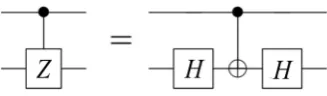
Figure 5. A controlled-Z gate in terms of a cNOT and two Hadamard gates.

Figure 6. A Toffoli gate implemented as the product of 1-qubit gates and cNOTs.

measurement in the computational basis is equivalent to a measurement in the X

[image:3.595.294.450.416.471.2] [image:3.595.290.454.513.561.2] [image:3.595.210.537.600.660.2]

(4)

0 1 0 1

,

2 2

 + − 

_{+ =} _{− =} 

 

 

 ,

and a _HS†_{gate is equivalent to a measurement in the}_Y_basis

0 1 0 1

,

2 2

y y

i i

 + − 

_{+ =} _{− =} 

 

 

 .

With these basic notions in mind, we have carried out several experiments and protocols: dense coding, quantum Fourier transforms, Bell’s inequality, Mermin’s inequalities (up to n = 5) and the construction of the prime state

3

p . The IBM Quantum Experience enables the simulation of the circuits prior to its actual implementation on the real quantum computer; this is helpful to ensure that the circuits are well designed. Each circuit has been run 5 times, each run comprising 8192 repetitions or shots. Mean results and standard deviations among the five runs have been calculated in all cases.

2. Implemented Experiments

2.1. Dense Coding

Dense coding is a protocol introduced by Bennett and Wiesner [24] that allows two bits of classical information to be transmitted between two partners (Alice and Bob) that share an EPR pair by performing local operations on just a single qubit (Alice’s) of the entangled pair, which is then eventually sent to Bob.

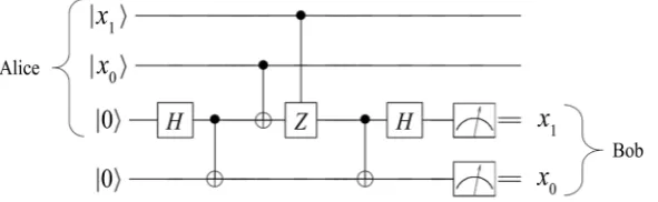
Dense coding can be implemented on the IBM 5Q using the circuit shown in

Figure 7, designed by Mermin [25]. The two uppermost horizontal wires in the circuit in Figure 7 represent the two classical bits that are to be sent by Alice (i.e.

{

0 , 1

}

i

x = ); this two bit string is generated using X gates (i.e.

0 1

1 0 x x 00

x x =X ⊗X _{). The two lowermost horizontal wires represent the}

qubits shared by Alice and Bob. The initial Hadamard gate and cNOT generate the entangled pair in the state

(

)

1 00 11 2

φ

+ ₌ ₊ _.

Then, the second cNOT and the controlled-Z implement the transformations of the protocol. Finally, the third cNOT and the last Hadamard gate transform the resulting Bell state into one of the four computational basis states before a joint measurement in this basis is carried out by Bob in order to obtain the information sent over by Alice.

The results obtained using the ibmqx 4 are shown in Table 1. The protocol is successfully completed around 83%, 74%, 78% and 75% of the times for the sequences 00, 01, 10 and 11, respectively.

(5)

[image:5.595.229.525.75.166.2]

[image:5.595.209.540.267.338.2]

Figure 7. Circuit for the implementation of dense coding.

Table 1. Mean probability outcomes (± standard deviation) of the dense-coding circuit

from Figure 7 after 5 runs of 8192 shots on the IBM 5Q computer (ibmqx 4), using qubits 3, 2, 1, 0. The column on the leftmost edge shows the 2-bit string transmitted by Alice and the uppermost row shows the possible outcomes after a joint measurement per-formed by Bob.

A\B 00 01 10 11

00 0.826 ± 0.003 0.041 ± 0.002 0.111 ± 0.004 0.023 ± 0.003 01 0.114 ± 0.007 0.744 ± 0.005 0.039 ± 0.003 0.101 ± 0.006 10 0.159 ± 0.025 0.025 ± 0.001 0.778 ± 0.025 0.038 ± 0.002 11 0.044 ± 0.005 0.097 ± 0.010 0.114 ± 0.003 0.746 ± 0.013

completed successfully with sufficiently high accuracy yet). It can be argued that superconducting qubits are not the ideal system to be sent over large distances, but then it should be considered how dense coding is going to be incorporated into a quantum computer that functions with superconducting qubits (if it is going to be so at all).

2.2. Quantum Fourier Transform

The quantum Fourier transform (QFT) is a basic unitary transformation in the field of Quantum Computation. For a given state of the computational basis

1 1 0

n

j ≡ j− ⋅⋅⋅j j , with ji=

{ }

0,1 , it is defined (in its product representation)

as:

(

2π0.0

)(

2π0.1 0

) (

2π0. 1 2 0

)

1 1 0 1 0 e 1 0 e 1 0 e 1 ,

2

n n

i j i j j i j j j

n _n

j j j − −

− ⋅⋅⋅ → + + ⋅⋅⋅ +  (1)

where 2

1 2 0 1 2 0

0. 2 2 2n

n n n n

j j− − j = j− + j− + + j represents a binary fraction. An efficient way of implementing the QFT for states of three qubits is shown in

Figure 8. To implement the circuit shown in Figure 8 on the IBM 5Q, we use the identity in Figure 9, where Rz

( )

λ

is a rotation of λ radians around the Z

axis on the Bloch sphere:

( )

1 0 .

0 e

z i

R

λ

 

≡  

  (2)

(6)

[image:6.595.241.511.77.161.2]

[image:6.595.223.515.202.258.2]

Figure 8. Circuit implementing the quantum Fourier transform of a state of three qubits.

Figure 9. Implementation of a controlled-Rz

( )

λ gate with 1-qubit gates and cNOTs.

each qubit), the state of every qubit can be taken to the closest of

{

+ −,

}

on the sphere. In this way, finally measuring in the X basis should result in a single three-bit string with probability equal to 1 in the ideal case.

For the 3-qubit case, the initial states chosen to be Fourier transformed are 000 and 011 . For the state 000 , the QFT—Equation (1)—gives the state:

(

)(

)

1 ₀ ₁ ₀ ₁ ₀ _{1 ,}

2 2 + + + (3) while the QFT of the state 011 gives:

(

)

(

3π 2

)(

3π 4

)

1 ₀ ₁ _{0 e} ₁ _{0 e} ₁

2 2

i i

− + + ₍₄₎

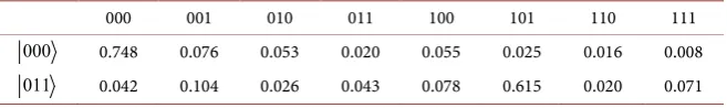
The results obtained for the two states (3) and (4) on the ibmqx 4 are shown in Table 2. Since, as explained above, the expected results are 000 and 101 with probability equal to 1 for the QFT of the states 000 and 011 respectively, it can be said that these states have been Fourier transformed with reliabilities of around 74.8 1.1%± _and 61.5 1.0%± _{(the errors are the standard deviations} among the 5 runs). QFTs of states of more than three qubits were not tried out because the limited connectivity among qubits (shown in Figure 1) would result in low-performance circuits.

Table 2. Mean probability outcomes of the Fourier transform of the states on the leftmost

column after 5 runs of 8192 shots on the IBM 5Q computer (ibmqx 4), using qubits 2, 1, 0 (standard deviations are not shown for the sake of clarity). Measurements were carried out in an appropriate basis so that the expected result is 000 for the state 000 and 101 for the state 011 , as explained in the text.

000 001 010 011 100 101 110 111

[image:6.595.211.540.671.720.2]

 

    ₍₆₎

where θ_{a b}__, is the angle between a and b. This means that the angles that

produce maximal violation of inequality (5) are θ_{a b}__,=θ_{b c}_,_=π3; that is, angles

of 60˚ between a b, and b c , , and 120˚ between

a c

 

,

(see Figure 10). According to Quantum Mechanics, the inequality should then be violated as 1.5 1 .

Bell’s inequality (5) can be tested on the IBM 5Q computers using the circuits shown in Figure 11. The Hadamard gate and cNOT in the circuits from Figure 11 generate the state ψ− _from ₁₁ _{. Then, the first circuit performs} measurements in the X basis (a) and in a basis whose vectors form a π 3 angle with those of the X basis (b), so it can be used to measure P a b

( )

, . The second and third circuits measure P a c

( )

 , and P b c

( )

 , , respectively. The results obtained using the ibmqx4 are shown in Figure 12.

The experimental values found for P a b

( )

, , P a c

( )

 , and P b c

( )

 , are [27]:

( )

, 0.392 0.014,

, 0.401 0.009,

, 0.389 0.012,

exp exp exp

P a b P a c P b c

= − ±

= ±

= − ±

   

  (7)

[image:7.595.293.458.595.697.2]

where P a b

( )

, is the sum of the probabilities of finding the results 00 or 11

(8)

[image:8.595.292.453.76.257.2]

DOI: 10.4236/jamp.2018.67123 1467 Journal of Applied Mathematics and Physics Figure 11. Circuits for measuring (1) P a b

( )

, (2) P a c

(

 ,

)

and (3) P b c

( )

 , .

[image:8.595.279.468.300.677.2]

Figure 12. Mean probability outcomes (±standard deviation) of circuits 1, 2, 3 from

Figure 11 after 5 runs of 8192 shots on the 5-qubit IBM computer (ibmqx 4), using qubits

(9)

DOI: 10.4236/jamp.2018.67123 1468 Journal of Applied Mathematics and Physics minus the probabilities of finding 01 or 10, and similarly for P a c

( )

 , and

( )

,

P b c  (note that the results according to Quantum Mechanics should be ±0.5). Hence, Bell’s inequality is violated:

1.182 0.020 1.± _ ₍₈₎

Other Bell-type inequalities can be tested on the IBM 5Q as well; for instance, the CHSH inequality [28] [29].

2.4. Mermin’s Inequalities

Mermin’s inequalities are a generalization of Bell-type inequalities for systems of more than two spin 1/2 particles (or qubits), derived in 1990 by Mermin [30]. The basic idea is that there exists an operator Mn (called a Mermin polynomial) whose quantum-mechanical expectation value exceeds the limits imposed by Local Realism for certain states. In this way, the incompatible predictions of the two theories can be experimentally tested and confronted: the inequalities must be fulfilled if Local Realism holds and violated in case Quantum Mechanics is correct.

The quantum-mechanical expectation value for Mn for some highly entangled states (GHZ-type states) exceeds the bounds imposed by Local Realism by an amount that grows exponentially with n (where n is the number of qubits). This fact implies that there is (in principle) no apparent limit to the amount by which Bell-type inequalities can be violated by certain entangled states. However, because the joint efficiency of n measurement apparatuses necessarily declines exponentially in n, and the n-qubit GHZ states are increasingly difficult to prepare as n grows, an exponentially greater violation of the inequalities for higher values of n will hardly be observed [30]. Mermin’s inequalities have been proposed as a figure of merit to assess the fidelity of a quantum computer [5]; in fact, they can be tested on the IBM 5Q computers for n=3,4,5_.

For n=3_{, a GHZ-type state and associated Mermin polynomial that give}

maximal violation of the corresponding inequality are:

(

)

2 1 0 2 1 0 2 1 0 2 1 0

3 3

1 000 111 , 2

, 2.

y x x x y x x x y y y y

i

M M ψ

σ σ σ σ σ σ σ σ σ σ σ σ

= +

= + + −

≤

(9)

For n = 4, those are [5]:

(

)

(

)

(

)

π4

3 2 1 0 3 2 1 0 3 2 1 0 3 2 1 0 4

3 2 1 0 3 2 1 0 3 2 1 0 3 2 1 0

3 2 1 0 3 2 1

1 0000 e 1111 , 2

i

y x x x x y x x x x y x x x x y y y x x y x y x y x x y x y y x x y x y x x y y y y y y x x x x

y y y x y y x

M ψ

σ σ σ σ σ σ σ σ σ σ σ σ σ σ σ σ

σ σ σ σ σ σ σ σ

= +

= + + +

+ + + +

+ + − −

−

(

+ 0 3 2 1 0 3 2 1 0

)

4

, 4.

y x y y y x y y y

M

σ σ σ σ σ σ σ σ

+ +

≤

(10)

DOI: 10.4236/jamp.2018.67123 1469 Journal of Applied Mathematics and Physics And for n = 5:

(

)

(

) (

4 3 2 1 0 4 3 2 1 0 4 3 2 1 0 4 3 2 1 0 5

4 3 2 1 0 4 3 2 1 0 4 3 2 1 0 4 3 2 1 0

4 3 2 1 0 4 3 2 1 0 4 3 2 1 0 4 1 00000 11111 ,

2

y x x x x x y x x x x x y x x x x x y x

x x x x y y y y x x y y x y x y y x x y

y x y y x y x y x y y x x y y x

i M

ψ

σ σ σ σ σ σ σ σ σ σ σ σ σ σ σ σ σ σ σ σ

σ σ σ σ σ σ σ σ σ σ σ σ σ σ σ σ σ

= +

= + + +

+ − + +

+ + + +

)

3 2 1 0

4 3 2 1 0 4 3 2 1 0 4 3 2 1 0 4 3 2 1 0

5

, 4.

y y y x

x y y x y x y x y y x x y y y y y y y y

M

σ σ σ

σ σ σ σ σ σ σ σ σ σ σ σ σ σ σ σ σ σ σ σ

+ + + +

≤

(11)

The circuits required for testing Mermin’s inequality for n = 3 and the choice of settings (9) are shown in Figure 13 (circuits for n = 4 and n = 5 are analogous). The Hadamard gate, cNOTs and S gate in Figure 13 generate the state

(

)

1 000 111

2 i

ψ

= + _.

Changing the position of the _S†_{gates in Circuit 1 from}_{Figure 13}_{allows to} measure 2 1 0

x y x

σ σ σ _and 2 1 0

x x y

σ σ σ _{. However, from our own results and those}

obtained in [5], it seems safe to assume symmetry under qubit exchange. That is:

2 1 0 2 1 0 2 1 0

y x x _exp x y x _exp x x y _exp

σ σ σ  σ σ σ  σ σ σ , and only one circuit is needed to

measure the three terms in the polynomial. The same is true for n = 4 and n = 5, which makes it possible to use a single circuit to measure all the terms with a same number of σys.

[image:10.595.278.470.516.691.2]

The experimental results obtained for the states and polynomials (9), (10) and (11) on the ibmqx 2 are collected in Table 3. These results show a clear violation of Mermin’s inequalities for n = 3, 4, 5. They can be compared to those found by Alsina and Latorre [5], also shown in Table 3 (the choice of state and polynomial for n = 5 is slightly different in [5], but completely equivalent to (11),

Figure 13. Circuits for testing Mermin’s inequality for n = 3: Circuit 1 measures

2 1 0

y x x

σ σ σ (YXX) and Circuit 2 measures 2 1 0

y y y

(11)

[image:11.595.209.540.127.194.2]

DOI: 10.4236/jamp.2018.67123 1470 Journal of Applied Mathematics and Physics Table 3. Comparison with the results obtained in [5] for Mermin’s inequalities. LR stands for Local Realism bound, QM for Quantum Mechanics bound, A-L for experimental re-sults obtained by Alsina and Latorre and GM-S for experimental rere-sults obtained in the present work.

LR QM A-L GM-S

3 qubits 2 4 2.85 ± 0.02 2.84 ± 0.07

4 qubits 4 8 2 4.81 ± 0.06 5.42 ± 0.04

5 qubits 4 16 4.05 ± 0.06 7.06 ± 0.03

since it has the same quantum-mechanical expectation value and Local Realism bound). We interpret the better results presented here to reflect the improvements of the IBM chips during the months in between both publications [31].

2.5. Prime State

The prime state pn is the superposition of all the computational-basis states

that correspond to prime numbers (written in binary format) up to a certain value _N₌2 1n₋ _[32]_:

( )

2 1

prime

1 _,

2

n

n _n

x

p x

π

−

∈

=

∑

₍₁₂₎

where

π

( )

x _{, known as the prime counting function, is the number of primes} less or equal than x. This state bears a large amount of entanglement [33]. The prime state for n = 3, i.e.

(

) (

)

3 1₂ 2 3 5 7 1₂ 010 011 101 111

p = + + + = + + + _,

can be created with the circuit shown in Figure 14.

The X gate acting on the first qubit ensures that all number states in the superposition created with the two Hadamard gates are odd: after these three gates have acted, the system is in the state

(

)

1 001 011 101 111 2

ψ = + + + _.

Thus, all that remains is converting the term 001 (1 is not a prime number) into 010 . This is achieved with the help of a Toffoli gate and a cNOT.

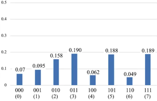
After implementing the circuit of Figure 14 for creating the prime state p3 on the ibmqx4, a joint measurement of the three qubits in the computational basis was carried out in order to assess the overall performance of the circuit. The results are shown in Figure 15.

The results show that, upon measurement of the purported prime state p3 , a prime number is obtained with probability 72.5 0.7%± _[34]_{. In this sense it} can be said that the prime state p3 has been constructed with an

approximated accuracy of 73%.

(12)

[image:12.595.305.448.76.150.2]

Figure 14. Circuit that creates the prime state p3 on the three uppermost qubits using

an ancilla.

Figure 15. Mean probability outcomes of joint measurements in the computational basis

of the three qubits of the purported prime state p3 after 5 runs of 8192 shots on the

5-qubit IBM quantum computer (ibmqx4), using qubits 2, 1, 0 (standard deviations are not shown for the sake of clarity).

they would allow to experimentally test, for instance, Riemann hypothesis–one of the mathematical problems of the millennium [33]. But in order to falsify Riemann hypothesis (or extend the limits of its validity) it is necessary to build superposition states of billions of prime numbers. Constructing the state p3 , even if this is not done by a general method for creating prime states, thus seems a modest first step.

Moreover, there exist a number of quantities in Number Theory that can surprisingly be measured experimentally on prime states [32]. The mean value of

1

z

σ

_is:

( )

4,1 4,3

1 1_,

z

N N

N

π

σ

[image:12.595.244.500.201.366.2]

(13)

DOI: 10.4236/jamp.2018.67123 1472 Journal of Applied Mathematics and Physics name is due to Pafnuty Chebyshev, who first noticed that the remainder upon dividing the primes by 4 gives 3 more often than 1).

Therefore, measuring the second qubit in the computational basis, and taking an outcome 0 as a 1 and an outcome 1 as a −1 when computing the mean value, give the Chebyshev bias, provided that

π

( )

N _{is known. For the state} p₃ created on the ibmqx 4, the experimental result for 1

z

σ _{obtained is:}

1 _{0.301 0.007,}

z exp

σ = − ± ₍₁₄₎

while the theoretical expected value for 1

z

σ _is:

1 _0.500,

z th

σ

= − ₍₁₅₎

which gives a relative error of around 40% in the measurement. Other quantities that can be measured experimentally on the prime state are:

( )

_{( )}

( )

_{( )}

( )

1 3 2 2

1 2 _, 1 2 1 2 4 _,

x x x y y

N N

π π

σ σ σ σ σ

π π

= + = ₍₁₆₎

where ( )1

( )

2 N

π

is the number of twin prime pairs

(

p p, +2

)

_{less or equal than}

N with p = 1 (mod 4) and ( )3

( )

2 N

2 N π2 N π2 N

∆ = − _.

The experimental results of the measurements of operators (16) on p3 on the ibmqx 4 are:

1

1 2 1 2

0.435 0.006,

0.641 0.022,

x exp

x x _{y y exp}

σ

σ σ σ σ

= ±

+ = ± (17) while the theoretical expected values are:

1 _0.500, 1 2 1 2 _1.000,

x _th x x y y _th

σ

=

σ σ

+

σ σ

= ₍₁₈₎

which give relative errors of approximately 13% and 36% respectively.

3. Conclusions

(14)

DOI: 10.4236/jamp.2018.67123 1473 Journal of Applied Mathematics and Physics in [5] that we interpret as a reflection of the improvements of the IBM quantum computers during the last months. Finally, the construction of the prime state

3

p has been carried out, which constitutes the first experimental realization of a prime state. Overall, the results obtained in these experiments, although moderately good in most cases, are still far from optimum.

Therefore, in light of these results, it is clear that there is still a lot of work to be done before a quantum computer can actually be useful for solving mathe-matical problems, simulating efficiently quantum systems, breaking classical en-cryption systems, etc. (in other words, fully achieve so-called quantum supre-macy [36]). But given the astounding pace at which technological developments are being push forward, it seems that the dream of building a functional univer-sal quantum computer within the next twenty years is close. Even more when one takes into account that it is likely (or at least plausible) that the full power of IBM quantum computers has not been shown yet for commercial reasons and thus it is not exhibited by the chips of the IBM Quantum Experience.

With no known fundamental obstacles on the way, quantum computers will surely end up being a reality in research centres all around the world. And, as it happens every time a new regime of Nature becomes experimentally available, a plethora of new discoveries will certainly accompany this “Second Quantum Revolution”. Meanwhile, proofs of principle like the ones presented here for several quantum circuits will be useful to help improving the systems.

Acknowledgements

We thank J.I. Latorre and D. Alsina for useful conversations. We also thank the IBM Quantum Experience for the use of the ibmqx2 and ibmqx4. G.S. acknowl-edges the grants FIS2015-69167-C2-1-P from the Spanish government, QUITEMAD+S2013/ICE-2801 from the Madrid regional government and SEV-2016-0597 of the Centro de Excelencia Severo Ochoa Programme.

References

[1] Nielsen, M.A. and Chuang, I.L. (2010) Quantum Computation and Quantum In-formation, Cambridge University Press, Cambridge.

https://doi.org/10.1017/CBO9780511976667

[2] Mermin, N.D. (2007) Quantum Computer Science. Cambridge University Press, Cambridge. https://doi.org/10.1017/CBO9780511813870

[3] The IBM Quantum Experience.

http://www.research.ibm.com/quantumhttp://www.research.ibm.com/quantum [4] Steffen, M., DiVincenzo, D.P., Chow, J.M., Theis, T.N. and Ketchen, M.B. (2011)

Quantum Computing: An IBM Perspective. Ibm Journal of Research and Develop-ment, 55, Paper 13. https://doi.org/10.1147/JRD.2011.2165678

[5] Alsina, D. and Latorre, J.I. (2016) Experimental Test of Mermin Inequalities on a Five Qubit Quantum Computer. Physical Review A, 94, Article ID: 012314. https://doi.org/10.1103/PhysRevA.94.012314

(15)

DOI: 10.4236/jamp.2018.67123 1474 Journal of Applied Mathematics and Physics Physical Review A, 94, arXiv:1605.05709v4.

[7] Berta, M., Wehner, S. and Wilde, M.M. (2016) Entropic Uncertainty and Measure-ment Reversibility. New Journal of Physics, 18, Article ID: 073004.

https://doi.org/10.1088/1367-2630/18/7/073004

[8] Rundle, R.P., Mills, P.W., Tilma, T., Samson, J.H. and Everitt, M.J. (2017) Quantum Phase Space Measurement and Entanglement Validation Made Easy. Physical Re-view A, 96, Article ID: 022117. https://doi.org/10.1103/PhysRevA.96.022117 [9] Hebenstreit, M., Alsina, D., Latorre, J.I. and Kraus, B. (2017) Compressed Quantum

Computation Using a Remote Five-Qubit Quantum Computer. Physical Review A, 95, Article ID: 052339. https://doi.org/10.1103/PhysRevA.95.052339

[10] Deffner, S. (2017) Demonstration of Entanglement Assisted Invariance on IBM’s Quantum Experience. Heliyon, 3, Article ID: e00444.

https://doi.org/10.1016/j.heliyon.2017.e00444

[11] Wootton, J.R. (2017) Demonstrating Non-Abelian Braiding of Surface Code Defects in a Five Qubit Experiment. Quantum Science and Technology, 2, No. 1.

[12] Sisodia, M., Shukla, A., Thapliyal, K. and Pathak, A. (2017) Design and Experimen-tal Realization of an Optimal Scheme for Teleportation of an n-Qubit Quantum State. Quantum Information Processing, 16, 292.

https://doi.org/10.1007/s11128-017-1744-2

[13] Sisodia, M., Shukla, A. and Pathak, A. (2017) Experimental Realization of Nonde-structive Discrimination of Bell States Using a Five-Qubit Quantum Computer.

Physics Letters A, 381, 3860-3874. https://doi.org/10.1016/j.physleta.2017.09.050 [14] Vuillot, C. (2017) Error Detection Is Already Helpful on the IBM 5Q Chip.

ar-Xiv:1705.08957.

[15] Michielsen, K., Nocon, M., Willsch, D., Jin, F., Lippert, T. and De Raedt, H. (2017) Benchmarking Gate-Based Quantum Computers. Computer Physics Communica-tions, 220, 44-55. https://doi.org/10.1016/j.cpc.2017.06.011

[16] Behera, B.K., Banerjee, A. and Panigrahi, P.K. (2017) Experimental Realization of Quantum Cheque Using a Five-Qubit Quantum Computer. arXiv:1707.00182. https://doi.org/10.1007/s11128-017-1762-0

[17] Kalra, A.R., Prakash, S., Behera, B.K. and Panigrahi, P.K. (2017) Experimental Demonstration of the No Hiding Theorem Using a 5 Qubit Quantum Computer. arXiv:1707.09462.

[18] Ghosh, D., Agarwal, P., Pandey, P., Behera, B.K. and Panigrahi, P.K. (2017) Auto-mated Error Correction in IBM Quantum Computer and Explicit Generalization. arXiv:1708.02297.

[19] Manabputra, G.S., Behera, B.K. and Panigrahi, P.K. (2017) Generalization and Par-tial Demonstration of an Entanglement Based Deutsch-Jozsa Like Algorithm Using a 5-Qubit Quantum Computer. arXiv:1708.06375.

[20] Yalçınkaya, İ. and Gedik, Z. (2017) Optimization and Experimental Realization of Quantum Permutation Algorithm. arXiv:1708.07900.

https://doi.org/10.1103/PhysRevA.96.062339

[21] Wootton, J.R. and Loss, D. (2017) A Repetition Code of 15 Qubits. ar-Xiv:1709.00990.

[22] Zhukov, A.A., Pogosov, W.V. and Lozovik, Y.E. (2017) Modeling Dynamics of En-tangled Physical Systems with Superconducting Quantum Computer. ar-Xiv:1710.09659.

(16)

Non-DOI: 10.4236/jamp.2018.67123 1475 Journal of Applied Mathematics and Physics

contextual Inequality Using IBM Quantum Computer. arXiv:1710.10717.

[24] Bennett, C.H. and Wiesner, S.J. (1992) Communication via One- and Two-Particle Operators on Einstein-Podolsky-Rosen States. Physical Review Letters, 69, 2881-2884. https://doi.org/10.1103/PhysRevLett.69.2881

[25] Mermin, N.D. (2002) Deconstructing Dense Coding. Physical Review A, 66, Article ID: 032308. https://doi.org/10.1103/PhysRevA.66.032308

[26] Bell, J.S. (1964) On the Einstein, Podolsky, Rosen Paradox. Physics, 1, 195-200. https://doi.org/10.1103/PhysicsPhysiqueFizika.1.195

[27] The errors have been calculated assuming the statistical independence of the va-riables summed: therefore, the variances have been added and then the square root was taken to obtain the standard deviation of the sum.

[28] Clauser, J.F., Horne, M.A., Shimony, A. and Holt, R.A. (1969) Proposed Experiment to Test Loal Hidden-Variable Theories. Physical Review Letters, 23, 880-884. https://doi.org/10.1103/PhysRevLett.23.880

[29] The IBM Quantum Experience.

https://quantumexperience.ng.bluemix.net/qx/tutorial?sectionId=full-user-guide&p age=003-Multiple_Qubits_Gates_and_Entangled_States2F050-Entanglement_and_ Bell_TestsFull User’s Guide/Entanglement and Bell Tests

[30] Mermin, N.D. (1990) Extreme Quantum Entanglement in a Superposition of Ma-croscopically Distinct States. Physical Review Letters, 65, 1838-1840.

https://doi.org/10.1103/PhysRevLett.65.1838

[31] In particular, we believe that the improvements in the violation of Mermin’s in-equalities are due to the availability of cNOTs among qubits 1,0 and 3,4, which were not present at the time Alsina and Latorre obtained their results. This interpretation is consistent with the fact that gate errors, readout errors, and decoherence and re-laxation times were similar in the present work and in [5], and with the fact that no improvement has been obtained for the 3-qubit case.

[32] Latorre, J.I. and Sierra, G. (2014) Quantum Computation of Prime Number Func-tions. Quantum Information and Computation, 14, Article ID: 0577.

[33] Latorre, J.I. and Sierra, G. (2015) There Is Entanglement in the Primes. Quantum Information and Computation, 15, 622-676.

[34] The error has been calculated as in Bell’s inequality.

[35] Rubinstein, M. and Sarnak, P. (1994) Chebyshev’s Bias. Exp. Math., 3, 173-197. https://doi.org/10.1080/10586458.1994.10504289