Optimal Bidding Strategy for Profit Maximization of
Generation Companies based on Whale Optimization
Algorithm in Day Ahead Market
Kavita Jain
M.Tech Scholar,YIT, Jaipur
Tanuj Manglani
Professor YIT, JaipurABSTRACT
In a deregulated electricity market, the aim of generating companies (GENCOs) is to maximize their profit by bidding optimally in the day-ahead market, under incomplete information of the competitors. This paper proposes a methodology to acquire the optimal bidding strategy of thermal GENCO in a uniform price spot market as a precise model of nonlinear operating cost function and minimum up/down constraints of unit commitment. Rivals bidding behavior is described using different probability distribution functions: normal, lognormal, gamma and weibull probability distribution function. Bidding strategy of a generator for each trading period in a day-ahead market is solved by whale optimization algorithm (WOA).WOA can dynamically monitor the repeatedly varying market demand and supply in each trading interval. This paper explores the effectiveness of the proposed algorithm with different probability functions to obtain optimal bid quantities and prices and compare the results.
General Terms
Electricity market, bidding strategies, whale optimization algorithm (WOA), Monte Carlo (MC) simulation, probability distribution
Keywords
The notations used in this paper are given below:
m ax
Q
Capacity of lth block of GENCO-R [MW].min
Q
Minimum output of lth block of GENCO-R [MW]. utl
M
Minimum up time of lth block of GENCO-G[hr]. dtl
M
Minimum down timeoflth block of GENCO-G[hr]. suc
h
Hot start-up cost [$], measured when unit has been shut down for a short time.sd c
c
Cold start-up cost [$], measured when unit has been shut down for a long time.T Cooling time constant [hr].
(t) on l
H
Number of hours the lth block of GENCO-R has been continuously ON at the end of hour t [hr].(t) off l
H
Number of hours the lth block of GENCO-R has been continuously OFF at the end of hour t [hr].l(t)
u
Binary variable, which is equal to 1, if the lth block is committed at hour t; otherwise, 0.off
T
Number of hours the unit has been OFF, at the time of startup [hr].1.
INTRODUCTION
Power industry switched to an open electricity marketfrom traditional monopoly system. In open electricity market independent system operator counterparts the hourly aggregate supply and forecasted demand to obtain hourly MCP. A GENCO, want to sell energy through this market, is enquired to bid blocks of power with prices for each trading period. For a GENCO, it is very essential to paradigm an optimal bidding strategy in order to maximize its profit. Each GENCO in the market tries to make their profit maximum and this form a competitive platform. This competitiveness in market maximize genco’s profit, reduces consumers payment and incentives investment. The main countenance of electricity market are limited number of competitors , very high cost of electricity stored in bulk amount, transmission constraints, demand-generation balance, grid reliability and stability,etc[1] which creates an oligopoly not a perfectly competitive market.
In a perfect competitive electricity market generating companies introduces a bidding price which makes its profit maximum. To maximize the profit the bidder has to bid their prices near to marginal production cost with the risk of losing the competition [1]. Wen et.al. Proposed Review on optimal bidding strategies in the electricity market. Higher bid means higher profit, therefore to decide the bidding price is a critical issue for GENCO’s. The main factors which helps in deciding the optimal bidding price of a GENCO’s know the technical, operating & regulatory constraints, own operating costs, and with an estimation of rival & market behavior. This is generally known as bidding strategy problem [2].
Dynamic programming approach was used to solve an optimal bidding problem for a single time period by David [3]. Huse et al. [4] have formulated a heuristic-based bidding strategy without involving the effect of inter-temporal constraints. Ma et al. [5] have created a stochastic optimization problem for the strategic bidding for a single period auction; MC simulation is used forestimation of competitors bidding behavior. H. Song et al. in [6], solved a multistage probabilistic bidding decision problem using Markov decision process.
formulation, due to their wide search capabilities [7], [8] and has been extended for spinning reserve market coordinated with energy market [9]. The strategic bidding problem, for a single period auction, can be modeled as a stochastic optimization problem and solved using GA based MC Approach [10]. Evolutionary Programming (EP) has also been applied for bidding strategy formulation in day ahead and reserve markets, using block bidding and considering unit operating constraints[11]. Fuzzy adaptive particle swarm optimization (PSO) has been explored for multi hourly trading, with dynamically changing load and generation [12]. Multi-objective PSO formulation can also be used to provide pareto-optimal solutions for maximizing producer profit, while minimizing the risk associated with price forecast uncertainty[13]. An opposition based on grey wolf optimizer is (OGWO) applied to maximize the profit of generator and the results are compared with other algorithms [23]. Grey wolf optimization (GWO) algorithm is used for profit maximization of generation companies under step-wise bidding protocol [24].
Meta-heuristic optimization algorithms are inspired by the nature thus they are becoming more and more popular in engineering applications. A new population based meta-heuristic optimization algorithm mimicking the hunting behavior of humpback whales named as Whale optimization algorithm. It was observed that WOA’s search agents tend to extensively search promising regions of design space and exploit the best one[14].
This paper proposes a new whale optimization approach to determine the optimal bidding strategy, in a day-ahead electricity market. Each Genco is assumed to bid in blocks, price and quantity pairs are submitted, with a sealed auction in a pay-as-bid mechanism. Rival bidding behavior is modeled using normal, lognormal, gamma and weibull probability distribution function which is constructed from historical market data analysis. Optimal bidding strategy for a generation company is, then, formulated as a stochastic problem and is transformed into an equivalent deterministic formulation using MC simulations.
In this work, the main contributions are as follows.
• Bidding strategies have been established for multi hourly trading in a day-ahead market using block bid model.
• Inter-temporal operating constraints [18] such as minimum up and down times have been assimilated.
• A sinusoidal nonlinear production cost and exponential start-up cost functions [19] have been accounted in the operating cost function. Though, any additional type of cost function can be simplyassimilated in the formulation.
• Rivals data with four different distribution functions has been generated.
• The problem for strategic bidding has been formulated in a dynamically varying environment, where both the load and generation variation frequently.
• WOA has been appropriately applied on the bidding problem to generate the optimal bid price and maximize the profit.
2.
PROBLEM DECRIPTION
We considered m+1 GENCOs, where m are the number of rival generatorsand m+1thGENCOis theGENCO-Rwhose
profit has to be maximized. In the electricity market all m+1 GENCOs submit their bid to the independent system operator (ISO).After getting the bidding prices from all GENCOs, ISO decides the market clearing price(MCP) as per the system demand.
GENCO-R and all rival generators can bid for maximum l blocks. Bidding in maximum blocks decreases the risk of financial loss to the generator. The size of rival’s bidding blocks are assumed to be known from the historical data and their bidding prices are calculated by probability distribution function (PDF) through of probability statistical analysis of historical bidding data.
In this paper we generate the input data using four different types of probability distribution functions, normal, lognormal, gamma &weibull. The mathematical expression which is used to generate the input data of all probability distribution functions are given below:
2.1 The Normal distribution
2 2
(P
)
1
(P )
exp
2(
)
2
m m
m l l
l m m
l l
µ
σ
σ
π
−
=
−
(1)Where
P
lmis the lth block bid price of mth rival.µ
lm,σ
lmare the mean value & standard deviation, respectively, of mth rival(lth block). Here we also generate the rivals bid price using different probability distribution functions. There is no loss of generality in generating data using other probability distributions [17].2.2 The Gamma distribution
A positive random variable X is said to be gamma(α, λ) distributed when it has the probability density
1
(t)
,
0
( )
tt
e
t
α α λλ
ρ
α
− −=
≥
Γ
(2)Where α>0 and λ>0 are the shape &scale parameter
respectively. The symbol
Γ α
( )
denotes the complete gamma function. The mean (D) and the squared coefficients of variation of a gamma (α,λ) distributed random variable X given by(X)
gamma
D
α
λ
=
AndV
x21
α
=
(3)
The gamma density is always unimodal; that is, the density has only one maximum at t= (α-1)/λ >0 and next decreases to
zero when t→∞, whereas for the case
V
x2≥
1 the identified variable has its maximum at t=0 and thus decreases from t=0 onwards. The failure rate function increases from zero to λ if2
V
x<
1
and decreases from infinity to zero ifV
x2>
1
.2.3 The weibull distribution
The positive random variable X is said to be weibull distributed when it has the probability density
1
(t)
( t)
exp[ ( t) ], t
0
Where α>0 is shape parameter & λ>0 is scale parameter.
The mean and squared coefficients of variation of the weibull random variable X are
1
1
(x)
1
weibullD
λ
λ
=
Γ
+
And2
2
(1 2 / )
1
[ (1 1/ )]
x
V
α
α
Γ +
=
−
Γ +
(5)The weibull density is always unimodal with maximum at
1 1/
(1 1 / )
t
=
λ
−−
α
α ifV
x2<
1
(
α
>
1
)
, and at t=0 if(
)
2
V
x<
1
α
≤
1
.The failure rate function increases from 0to infinity if
V
x2<
1
and decreases from infinity to zero if 2V
x>
1
.2.4 The lognormal distribution
The lognormal has shape parameter α>0 and the scale parameter λ may assume each real value. The mean and the squared coefficient of variation of the lognormal distribution are given by
2 log
1
exp
2
nD
=
λ
+
α
And2 2
exp(
) 1
x
V
=
α
−
(6)
The lognormal density is also unimodal with a maximum at t=exp(λ-α2).The failure rate function first increase after that it decreases to zero when t→∞ and thus the failure rate only decreases in long life range. The weibull and gamma densities
are similar in shape and for
V
x2<
1
the lognormal density takes on shape similar to the weibull and gamma densities.For the case
V
x2≥
1
the weibull and gamma densities have their maximum value at t=0; most outcomes tend to be small and very large outcomes occur only occasionally. The difference between normal, gamma, weibull and lognormal densities become most significant in their tail behavior.Once a unit is committed/decommitted, there is a predefined minimum time after which it can be decommitted/committed again. These inter-temporal operating constraints of GENCO-R, such as minimum up & down times have been reflected in the present work. Ramp up/down rates, are assumed sufficiently high/low for all the blocks of GENCO-R. The size of any block during each hour is limited by its generation limits and not by its ramp up/down rates. Hence, the ramp rate constraints are disregarded in the formulation.
Considering non differentiable, non convex production cost
function
c
l(t)pr , nonlinear (exponential) start-up cost function sul
c
and constant shut-down costc
sdl , the operating costfunction
c
l(t)for the lth block of GENCO-R can be written asl(t) l(t)
{
l(t)(1 u
l(t 1))} c {(1
l(t)) u
l(t 1)}
pr su sd
l l
c
=
c
+
c
u
−
−+
−
u
−(7)
Where
2
l(t) 0
(Q )
l(t) 1(Q )
l(t)c
2 4sin(c Q
4 minQ ))
l(t) prc
=
c
+
c
+ +
c
−
(8)
1 exp
offsu su sd
l c c
T
c
h
c
T
−
=
+
−
(9)For the large thermal generators, input-output characteristics are not always smooth due to sequential initial of multi-number of valves to gain ever-increasing output of the unit[19].Normally, as each steam admission valve in a turbine starts to open, it creates a rippling effect on the unit curve. This rippling effect of valve point loading has been shown as a recurring rectified sinusoidal function in [20]. Result of valve point loading on economic dispatched output of units is previously established in [21], which resolves the significance of precise production cost function application in strategic bidding. Equation (9) represents this sinusoidal nonlinear function, where c0,c1, &c2 are cost coefficients and c3& c4 are
the constants of the valve point loading effect. An exponential function is considered in (22), to represent the relationship between the start-up cost & the shut off time. Though, any existing start-up cost function can be used. The cost acquired in start-up & start-down are united in the operating cost function so that the real benefit is considered and the units are committed/decommitted accordingly.
The optimal bidding strategy of GENCO-R can be formulated as profit maximization profit in terms of dispatched power output (
Q
l(t)) and MCP (MCP
(t)). The product of dispatched power and MCP gives the revenue obtained. The cumulative profit for lth blocks of the generator over time period “T” is expressed as(t)
(t) l(t) (t) l(t) (t) 1 1
(M C P , Q ) (M C P Q )
L
T L
l
P t l
f c
M axim ize
= =
=
∑ ∑
∗ −(10)
Subject to constraints
1) Generation limits
min l(t) l(t) max l(t)
,
Q u
≤
Q
≤
Q
u
∀ ∈
t
T
.
(11)2) Minimum up time
l(t 1) (t)
(1
−
u
+)
M
lut≤
H
lon,
if
u
l(t)=
1.
(12)3) Minimum down time
(t 1) (t)
,
dt off
l l l
u
+M
≤
H
if
u
l(t)=
0.
(13)4) Limitations on bid price
(t) (t)
,
l l
c
≤
p
≤
p
∀ ∈
t
T
.
(14)The optimization problem defined in (10)-(14) can be solved to obtain the optimal block bid price of the lth block of
GENCO-R at hour t, represented as
p
l(t) . In (10),p
l(t)&P
ml do not explicitly appear, but these are implicitly included in the process of determining MCP. Equation (11)-(13) are the operating constraints, whereas (14) resembles to the bid price
cap, i.e.,
p
.of the optimal bidding strategy for GENCO R, with objective function (7) and constraints (12)-(15), be remodeled a stochastic optimization problem, to be solved by MC based WOA.
3.
PROPOSED SOLUTION
ALGORITHM
The problem formulated in previous section has been solved by using Monte Carlo approach; a technique which obtain a probabilistic approximation of a mathematical problem by using statistical sampling. This approach runs stochastic simulation using random numbers and simultaneously calculates the equation to reach at a solution. This MC simulation is integrated with, a new population–based meta-heuristic whale optimization algorithm (WOA), to obtain the optimal bidding strategy for a GENCO.
3.1
Monte Carlo Approach
MC approach proceeds as follows:
• Generate a large number of random samples of block bid prices for all the rivals, considering their PDFs.
• Obtain large trial outcomes, by solving the optimization problem with sample values of block bid prices for all the rivals.
• Calculate the expectation value, taking average of all the trial outcomes.
Details of algorithm:
1. Specify the number of Monte Carlo simulations allowed, M.
2. Set simulation counter mc=0.
3. Create random values of bid prices
P
lmfor each lth block of m rivals using normal, gamma, weibull &lognormal distribution function.4. Use WOA to search optimal bid price for each lth block
of GENCO-R and record optimal the value of
p
lmc(t).5. Set simulation counter mc=0.
6. Create random values of bid prices
P
lmfor each lth blockof m rivals using normal, gamma, weibull &lognormal distribution function.
7. Use WOA to search optimal bid price for each lth block
of GENCO-R and record optimal the value of
p
lmc(t).8. Update mc=mc+1.
9. If mc<MC then go to (step 3), else go to (step 7).
10. Determine thepredictablevalue of optimal bid price that
is the average of
p
lmc(t)(mc=1,2,….MC). This value is theoptimal bidding price(pl(t)) for lth block of GENCO-R at
hour t.
3.2 Whale Optimization Algorithm
A new optimization algorithm known as whale optimization algorithm [14] has been introduced to metaheuristic algorithm by Mirjalili and Lewis. The whales are considered to be as intelligent mammals with emotion. The WOA is inspired by the unique hunting behavior of humpback whales. The nature of humpback whale is to hunt krill’s or small fishes which are near to the surface of sea shown in fig.1. A special hunting technique is used by humpback whales called bubbles net feeding method. In this technique they swim around the prey and make distinctive bubbles along a circle or 9-shaped path.
Fig.1. bubble-net feeding behavior of humpback whales
The mathematical model of WOA is described in the following sections:
1. Encircling the prey
2. Bubble net hunting method
3. Search for prey
3.2.1 Encircling the Prey
Humpback whales can find out the prey location and encircle them. WOA assumes that the present best candidate solution is the goal prey or is near to the optimum. The other search agents try to update their positions toward best search candidate. The behavior modeled is as
.X *(t)
(t)
D
=
C
−
X
ur
ur uur
uur
(15)
(t 1)
X*(t)
.
X
+ =
−
A D
uur
uur
ur ur
Fig.2. 2D and 3D position vectors and their possible next locations (X* is the best solution obtained so far)
Fig.3.bubble-net search mechanism implemented in WOA (X* is the best solution obtained so far):(a)shrinking encircling mechanism and (b)spiral updating position.
Where t is the current iteration,
A
ur
and
C
ur
is coefficient
vectors
X*(t)
uur
is the position vector of the best solution
obtained so far
X
(t)
uur
is the position vector. ll is the absolute value and . is the element by element multiplication.
It is worth to mention here that X* should be updated in each iteration if there is a better solution.
The vectors A and C are calculated as follows:
2 .
A
=
a r
−
a
r
r r
r
(17)
2
C
r
→ →
=
(18)Where
α
uv
is linearly decreased from 2 to 0 over the course of iterations (in both exploration and exploitation phases) and r is a random vector in [0, 1].
Fig.2(a) illustrates the basis behind equation (16) for a 2D problem. The position (X.Y) of a search agent can be updated according to the position of the current best record(X*,Y*).the possible updating position of a search agent in 3D space is also depicted in fig.2(b). It should be noted that by defining
the random vector (
r
→) it is possible to search any position in the search space located between the key-points shown in fig.3.
3.2.2 Bubble- net hunting method (exploitation
phase)
In the bubble net hunting method two approaches are used:
(I) Shrinking encircling prey is achieved by decreasing the
value of
a
→in equation (17) thus the range of
A
→is also
decreased.
A
→is a random value in the interval [-α,α] where α is decreased from 2 to 0 over the course of
iterations. Setting random values for
A
→in [-1, 1], the new position of search agent is defined anywhere between the original and current best agent represented in fig.3(a).
(II) Spiral position update approach first calculates the
'
(t 1)
. .cos(2 )
bt*( )
X
+ =
D e
π
l
+
X
t
uur
uur
uuur
(19)
( )
*
(t)
D
=
X
t
−
X
r
r
r
(20)
Where b is constant and l is random number in [-1,1]
The mathematical model is as follows:
(t 1)
rand.
X
+ =
X
−
A D
uur
uur
ur ur
if P<0.5 (21)
'
(t 1)
. .cos(2 )
bl*( )
X
+ =
D e
π
l
+
X
t
uur
uur
uuur
if P≥0.5 (22)
Where P is the random number of [0,1]
3.2.3 Search for prey (exploration phase)
Humpback whale arbitrarily searches according to the
position of each other. Therefore we use
A
ur
with the random
values between -1 to 1. This mechanism
A
>
1
ur
highlights
exploration and allows the WOA to perform a global search. The mathematical model is as follows:
.X
randD
=
C
−
X
ur
ur ur
uur
(23)
(t 1)
X
rand.
X
+ =
−
A D
uur
ur
ur ur
(24)
Here,
X
randuur
is random position vector selected from the current population.Selected of possible positions nearby a
particular solution with
A
>
1
ur
are shown in fig.4.
Fig.4 Bubble net search spiral updating position mechanism
4.
RESULTS AND DISCUSSION
The effectiveness of the proposed optimal bidding strategy using WOA has been demonstrated on a numerical example based on problem formulated in section II. This problem is
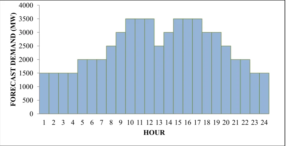
formulated in a dynamically changing environment and bidding strategies are developed for multi-hourly trading ii a day-ahead market. A daily load curve for 24hrs is shown in the fig. 5
Normal probabilitydistribution parameters of rivals block bid prices (shown in Table 1) are taken in such a manner that each block has a exclusive pdf. The parameters of all three power blocks of GENCO-R are shown in Table 2.
At the beginning of first hour, blocks 1, 2, and 3 of GENCO-R are supposed to be ON, ON, and OFF, respectively. The maximum no. of MC simulation iterations is taken as 10000 and in each iteration. The bid price for each hour and each block of GENCO-R is obtained using WOA search technique. The optimal bid price is the average value of these 10000 random samples of bid prices. Table 3 shows the dispatched and non-dispatched powers of GENCO-R and rivals during every trading period. Dispatched power output (in boldface) denotes the minimal block (output) in that particular hour and ND stands for no-dispatch of that block. The following observations can be made from the results shown in Table 3.
• Block 3 of generator-R is not committed in the hours of negative benefit (from 1 to 9 hr) because of its great production cost and small system demand.
• Cold start-up cost is accounted in the production cost of block 3, when it is committed at 10 hr, because it has been shut down for a long time (9 hr).
• At the end of 12 hr, block 3 is again not committed due to smallsystem demand, & minimum down time constraint is active from 13 to 14 hr.
• Block 3 is recommitted at 15 hr, and hot start-up cost is accounted in the production cost of this hour, because it has been shut down for a short time (2 hr).
• Block 3 is again not committed from 21 to 24 hr due to low system demand.
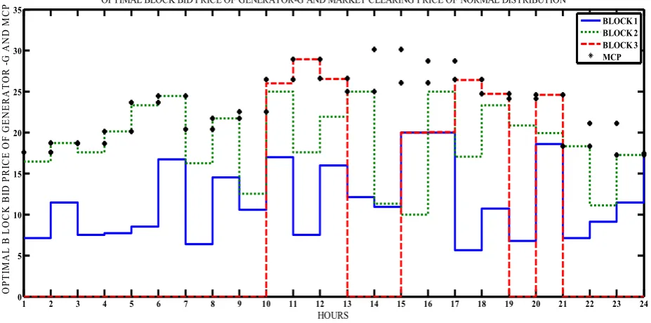
Optimal bid prices of each trading hour for blocks 1, 2, and 3 of GENCO-R are closely following each other to maximize the profit as depicted in Fig. 7. The MCP for each trading hour is also shown in Fig. 7.MCP for 5, 6, 7, 9, 14, 21, 22 hr is higher than optimal block bid price of GENCO-R, and no block of GENCO-R is selected as marginal block in these hours. It should be noted that optimal bid price must be less than or equal to the marginal bid price at any hour for successful dispatch of a block. Optimal bid price of block 3 is shown zero during 1-9 hr, 13-14 hr, & 21-24 hr, when it is not committed.
Fig.5 Power Load Forecast by System Operator
Table 1.Data of Rival’s Bidding Parameters
BLOCK 1 BLOCK 2 BLOCK 3
Qlm µlm σlm Qlm µlm σlm Qlm µin σlm
RIVAL 1 (n=1) 200 10 2.5 300 20 3 400 30 3
RIVAL 2 (n=2) 300 15 3 400 30 2 500 50 4
RIVAL 3 (n=3) 250 10 2 300 15 2.5 300 20 2.5
[image:7.595.64.537.541.685.2]RIVAL 4 (n=4) 300 20 4 350 25 5 450 40 5
Table 2. Data of GENCO-R Power Blocks
C0
(MW2h)
C1($/
MWh )
C2
($/h) C3
($/h)
C4(ra
d./M W)
Qmax
(M W)
Qmin
(M W)
MUT (h)
MD T (h)
h ($)
δ ($)
τ
(h )d i
c
($)
Block1 0.00482 7.97 78 150 0.063 200 50 1 1 1000 1500 1 100
Block2 0.00194 15.85 310 200 0.042 400 100 2 1 1500 2500 1 200
Block3 0.001562 32.92 561 300 0.0315 600 100 4 2 2000 4000 8 400
0
500
1000
1500
2000
2500
3000
3500
4000
1 2 3 4 5 6 7 8 9 10 11 12 13 14 15 16 17 18 19 20 21 22 23 24
F
O
R
E
C
A
S
T
D
E
M
A
N
D
(
M
W)
Table 3.Dispatched Power Output of GENCO–R and Rivals using normal distribution
Fig.6.Optimal Block Bid Price of Generator-R And Market Clearing Price Of Normal Distribution
B1 B2 B3 B1 B2 B3 B1 B2 B3 B1 B2 B3 B1 B2 B3
200 300 250 300 200 300 400 300 350 400 400 500 300 450 600
1 1500 200 300 ND 300 ND ND ND 100 ND ND ND ND 200 400 ND
2 1500 200 ND ND 300 ND ND 100 300 ND ND ND ND 200 400 ND
3 1500 200 300 ND 300 ND ND ND 300 ND ND ND ND 200 200 ND
4 1500 200 ND ND 300 ND ND ND 300 ND 300 ND ND 200 200 ND
5 2000 200 300 ND 300 ND ND 250 300 ND ND 50 ND 200 400 ND
6 2000 200 ND ND 300 ND ND 250 300 ND 300 50 ND 200 400 ND
7 2000 200 ND ND 300 ND ND 250 300 ND ND 350 ND 200 400 ND
8 2500 200 300 ND 300 ND ND 250 300 ND 300 250 ND 200 400 ND
9 3000 200 300 400 300 50 ND 250 300 300 300 ND ND 200 400 ND
10 3500 200 300 ND 300 400 ND 250 300 300 300 350 ND 200 400 200
11 3500 200 300 400 300 400 ND 250 300 300 300 ND ND 200 400 150
12 3500 200 300 400 300 ND ND 250 300 300 300 350 ND 200 400 200
13 2500 200 300 ND 300 ND ND 250 300 ND 300 250 ND 200 400 ND
14 3000 200 300 400 300 ND ND 250 300 300 300 50 ND 200 400 ND
15 3500 200 300 400 300 ND ND 250 300 300 300 350 ND 200 400 200
16 3500 200 300 ND 300 ND ND 250 300 300 300 350 ND 200 400 200
17 3500 200 300 200 300 400 ND 250 300 300 300 350 ND 200 400 ND
18 3000 200 300 400 300 ND ND 250 300 ND 300 350 ND 200 400 ND
19 3000 200 300 ND 300 ND ND 250 300 ND 300 350 ND 200 400 400
20 2500 200 300 ND ND ND ND 250 300 300 300 250 ND 200 400 ND
21 2000 200 50 ND 300 ND ND 250 300 ND 300 ND ND 200 400 ND
22 2000 200 ND ND 300 ND ND 250 300 300 50 ND ND 200 400 ND
23 1500 200 ND ND 300 ND ND 250 300 ND ND ND ND 200 250 ND
24 1500 200 ND ND 300 ND ND 250 300 ND 250 ND ND 200 250 ND LOAD DISPATCH OF NORMAL DISTRIBUTION OF 5 GENCO AND 3 BLOCK
HOUR LOAD
Rival 1 Rival 2 Rival 3 Rival 4 GENCO-R
1 2 3 4 5 6 7 8 9 10 11 12 13 14 15 16 17 18 19 20 21 22 23 24
0 5 10 15 20 25 30 35
HOURS
O
P
T
IM
A
L
B
L
O
C
K
B
ID
P
R
IC
E
O
F
G
E
N
E
R
A
T
O
R
-G
A
N
D
M
C
P OPTIMAL BLOCK BID PRICE OF GENERATOR-G AND MARKET CLEARING PRICE OF NORMAL DISTRIBUTION
[image:8.595.65.529.503.733.2]Table 4. Dispatched Power Output of GENCO–R and Rivals using lognormal distribution
Fig.7. Optimal Block Bid Price of Generator-R And Market Clearing Price Of Lognormal Distribution
B1 B2 B3 B1 B2 B3 B1 B2 B3 B1 B2 B3 B1 B2 B3
200 300 250 300 200 300 400 300 350 400 400 500 300 450 600
1 1500 200 300 ND 300 ND ND ND 100 ND ND ND ND 200 400 ND
2 1500 200 ND ND 300 ND ND 100 300 ND ND ND ND 200 400 ND
3 1500 200 300 ND 300 ND ND ND 300 ND ND ND ND 200 200 ND
4 1500 200 ND ND 300 ND ND ND 300 ND 300 ND ND 200 200 ND
5 2000 200 300 ND 300 ND ND 250 300 ND ND 50 ND 200 400 ND
6 2000 200 ND ND 300 ND ND 250 300 ND 300 50 ND 200 400 ND
7 2000 200 ND ND 300 ND ND 250 300 ND ND 350 ND 200 400 ND
8 2500 200 300 ND 300 ND ND 250 300 ND 300 250 ND 200 400 ND
9 3000 200 300 400 300 50 ND 250 300 300 300 ND ND 200 400 ND
10 3500 200 300 ND 300 400 ND 250 300 300 300 350 ND 200 400 200
11 3500 200 300 400 300 400 ND 250 300 300 300 ND ND 200 400 150
12 3500 200 300 400 300 ND ND 250 300 300 300 350 ND 200 400 200
13 2500 200 300 ND 300 ND ND 250 300 ND 300 250 ND 200 400 ND
14 3000 200 300 400 300 ND ND 250 300 300 300 50 ND 200 400 ND
15 3500 200 300 400 300 ND ND 250 300 300 300 350 ND 200 400 200
16 3500 200 300 ND 300 ND ND 250 300 300 300 350 ND 200 400 200
17 3500 200 300 200 300 400 ND 250 300 300 300 350 ND 200 400 ND
18 3000 200 300 400 300 ND ND 250 300 ND 300 350 ND 200 400 ND
19 3000 200 300 ND 300 ND ND 250 300 ND 300 350 ND 200 400 400
20 2500 200 300 ND ND ND ND 250 300 300 300 250 ND 200 400 ND
21 2000 200 50 ND 300 ND ND 250 300 ND 300 ND ND 200 400 ND
22 2000 200 ND ND 300 ND ND 250 300 300 50 ND ND 200 400 ND
23 1500 200 ND ND 300 ND ND 250 300 ND ND ND ND 200 250 ND
24 1500 200 ND ND 300 ND ND 250 300 ND 250 ND ND 200 250 ND LOAD DISPATCH OF LOGNORMAL DISTRIBUTION OF 5 GENCO AND 3 BLOCK
HOUR LOAD
Rival 1 Rival 2 Rival 3 Rival 4 GENCO-R
1 2 3 4 5 6 7 8 9 10 11 12 13 14 15 16 17 18 19 20 21 22 23 24
0 5 10 15 20 25 30 35
HOURS
O
P
T
IM
A
L
B
L
O
C
K
B
ID
P
R
IC
E
O
F
G
E
N
E
R
A
T
O
R
-G
A
N
D
M
C
P OPTIMAL BLOCK BID PRICE OF GENERATOR-G AND MARKET CLEARING PRICE OF LOGNORMAL DISTRIBUTION
[image:9.595.67.534.508.739.2]Table 5.Dispatched Power Output of GENCO–R and Rivals using weibull distribution
Fig.8.Optimal Block Bid Price of Generator-R and Market Clearing Price Of Weibull Distribution
B1 B2 B3 B1 B2 B3 B1 B2 B3 B1 B2 B3 B1 B2 B3
200 300 250 300 200 300 400 300 350 400 400 500 300 450 600
1 1500 200 ND ND 300 ND ND 250 300 ND ND ND ND 200 250 ND
2 1500 200 ND ND 300 ND ND 250 300 ND ND ND ND 200 250 ND
3 1500 200 ND ND 300 ND ND 250 300 ND ND ND ND 200 250 ND
4 1500 200 ND ND ND ND ND 250 300 150 ND ND ND 200 400 ND
5 2000 200 ND 300 300 ND ND 250 300 ND 50 ND ND 200 400 ND
6 2000 200 ND ND 300 ND ND 250 300 50 300 ND ND 200 400 ND
7 2000 200 300 ND 300 ND ND 250 300 300 ND ND ND 200 150 ND
8 2500 200 300 ND 300 ND ND 250 300 300 300 ND ND 200 350 ND
9 3000 200 300 ND 300 ND ND 250 300 ND 300 350 ND 200 400 400
10 3500 200 300 400 300 ND ND 250 300 300 300 350 ND 200 400 200
11 3500 200 300 200 300 400 ND 250 300 300 300 350 ND 200 400 ND
12 3500 200 300 ND 300 ND ND 250 300 300 300 350 ND 200 400 600
13 2500 200 300 ND 300 ND ND 250 300 300 300 ND ND 200 350 ND
14 3000 200 300 100 300 ND ND 250 300 300 300 350 ND 200 400 ND
15 3500 200 300 400 300 200 ND 250 300 300 300 350 ND 200 400 ND
16 3500 200 300 ND 300 400 ND 250 300 300 300 350 ND 200 400 200
17 3500 200 300 ND 300 400 ND 250 300 300 300 350 ND 200 400 200
18 3000 200 300 ND 300 ND ND 250 300 300 300 350 ND 200 400 100
19 3000 200 300 ND 300 ND ND 250 300 300 300 350 ND 200 400 100
20 2500 200 300 ND 300 ND ND 250 300 300 300 ND ND 200 350 ND
21 2000 200 300 ND 300 ND ND 250 300 ND 300 ND ND 200 100 ND
22 2000 200 ND ND 300 ND ND 250 300 ND 300 ND ND 200 400 ND
23 1500 200 ND ND 300 ND ND 250 300 ND ND ND ND 200 250 ND
24 1500 200 ND ND 300 ND ND 250 300 ND ND ND ND 200 250 ND LOAD DISPATCH OF WEIBULL DISTRIBUTION OF 5 GENCO AND 3 BLOCK
HOUR LOAD
Rival 1 Rival 2 Rival 3 Rival 4 GENCO-R
1 2 3 4 5 6 7 8 9 10 11 12 13 14 15 16 17 18 19 20 21 22 23 24
0 5 10 15 20 25 30 35
HOURS
O
P
T
IM
A
L
B
L
O
C
K
B
ID
P
R
IC
E
O
F
G
E
N
E
R
A
T
O
R
-G
A
N
D
M
C
P OPTIMAL BLOCK BID PRICE OF GENERATOR-G AND MARKET CLEARING PRICE OF WEIBULL DISTRIBUTION
Table 6.Dispatched Power Output of Generator –R and Rivals using gamma distribution
Fig.9. Optimal Block Bid Price of Generator-R and Market Clearing Price Of Gamma Distribution
B1 B2 B3 B1 B2 B3 B1 B2 B3 B1 B2 B3 B1 B2 B3
200 300 250 300 200 300 400 300 350 400 400 500 300 450 600
1 1500 200 ND ND 150 ND ND 250 300 ND ND ND ND 200 400 ND
2 1500 200 ND ND ND ND ND 250 300 ND 150 ND ND 200 400 ND
3 1500 200 ND ND 300 ND ND 250 300 ND ND ND ND 200 250 ND
4 1500 200 ND ND 300 ND ND 250 300 ND ND ND ND 150 300 ND
5 2000 200 300 ND 300 ND ND 250 300 50 ND ND ND 200 400 ND
6 2000 200 ND ND 300 ND ND 250 300 50 300 ND ND 200 400 ND
7 2000 200 300 ND 300 ND ND 250 300 ND 50 ND ND 200 400 ND
8 2500 200 250 ND 300 ND ND 250 300 200 300 350 ND 200 400 ND
9 3000 200 300 100 300 ND ND 250 300 300 300 350 ND 200 400 ND
10 3500 200 300 400 300 200 ND 250 300 300 300 350 ND 200 400 ND
11 3500 200 300 400 300 200 ND 250 300 300 300 350 ND 200 400 ND
12 3500 200 300 400 300 200 ND 250 300 300 300 350 ND 200 400 ND
13 2500 200 300 ND 300 ND ND 250 300 300 300 ND ND 200 50 ND
14 3000 200 300 ND 300 ND ND 250 300 300 300 350 ND 200 400 100
15 3500 200 300 200 300 400 ND 250 300 300 300 350 ND 200 400 ND
16 3500 200 300 400 300 200 ND 250 300 300 300 350 ND 200 400 ND
17 3500 200 300 400 300 200 ND 250 300 300 300 350 ND 200 400 ND
18 3000 200 300 ND 300 100 ND 250 300 300 300 350 ND 200 400 ND
19 3000 200 300 100 300 ND ND 250 300 300 300 350 ND 200 400 ND
20 2500 200 300 ND 300 ND ND 250 300 250 300 ND ND 200 400 ND
21 2000 200 300 ND 300 ND ND 250 300 150 300 ND ND 200 ND ND
22 2000 200 ND ND 300 ND ND 250 300 ND ND 350 ND 200 400 ND
23 1500 200 ND ND 300 ND ND 250 300 ND ND ND ND 200 250 ND
24 1500 200 ND ND 300 ND ND 250 300 ND ND ND ND 200 250 ND LOAD DISPATCH OF GAMMA DISTRIBUTION OF 5 GENCO AND 3 BLOCK
HOUR LOAD
Rival 1 Rival 2 Rival 3 Rival 4 GENCO-R
1 2 3 4 5 6 7 8 9 10 11 12 13 14 15 16 17 18 19 20 21 22 23 24
0 5 10 15 20 25 30
HOURS
O
P
T
IM
A
L
B
L
O
C
K
B
ID
P
R
IC
E
O
F
G
E
N
E
R
A
T
O
R
-G
A
N
D
M
C
P
OPTIMAL BLOCK BID PRICE OF GENERATOR-G AND MARKET CLEARING PRICE OF GAMMA DISTRIBUTION
Fig.10.Hourly Profit of all Four Distributions
Fig.11. Total Profit of 24 Hours using Different Distributions
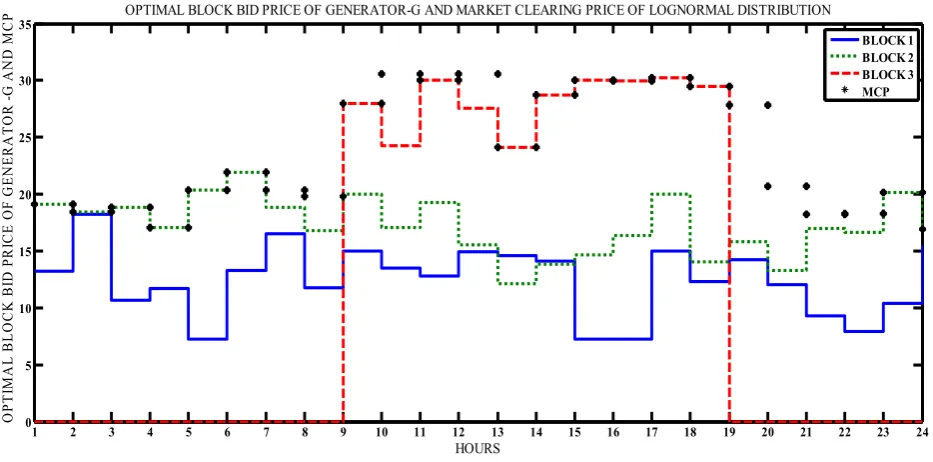
The load dispatch with lognormal probability distribution for 4 rivals in 3blocks for 24hrs is shown in table 4 and block bid curve with MCP of GENCO-R using lognormal distribution is shown in fig.7.
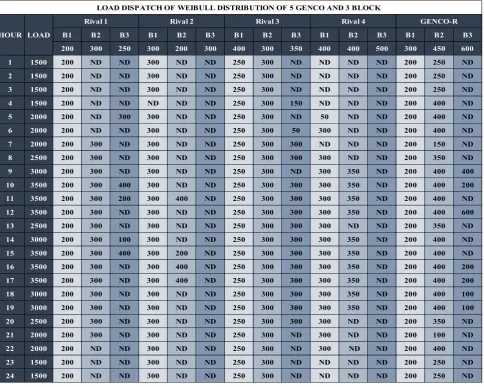
The load dispatch for weibull probability distribution for 4 rivals in 3blocks for 24hrs is shown in table 5and block bid curve with MCP of GENCO-R using weibull distribution is shown in fig.8.
The load dispatch with gamma probability distribution for 4 rivals in 3blocks for 24hrs is shown in the table 6and block bid curve with MCP of GENCO-R using gamma distribution is shown in fig.7.
Fig.10 shows the profit of Genco-R for 24 hour in a day ahead market for all the distributions which are discuss before. Total profit of Genco-R for different probability distribution shown in Fig.11. Here we see that the total profit comes obtained by using lognormal probability distribution is maximum. This result shows the superiority to lognormal distribution above other distribution.
5.
CONCLUSION
Restructuring in electricity market gives a platform to GENCO’s to compete with other rivals and to minimize the electricity price for consumers. In such a vigorous market model, Genco frame a bidding strategy to maximize their profit by bidding in a pool market without knowing the information regarding other rivals. To solve the problem, this paper has presented an optimal bidding strategy based on WOA for GENCO-R.
The conclusions are as follows:
1. Rivals’ bidding prices have been represented as stochastic variables with normal, lognormal, gamma and weibull probability distributions. A stochastic optimization model for the formulation of optimal bidding decision has been established and solved by MC simulation.
2. The above analysis shows that the lognormal distribution is most appropriate for this data set. The superiority of lognormal probability distribution has been successfully tested over normal, gamma and weibull probability distribution using WOA approach for multi-hourly market clearing simulation cases. In successive 24-h market clearing
2 4 6 8 10 12 14 16 18 20 22 24
0 5000 10000 15000
HOUR(hr)
P
R
O
F
IT
(M
W
h
/$
)
PROFIT OF WOA WITH DIFFERENT DISTRIBUTION IN DAY AHEAD MARKET
WEIBULL LOGNORMAL NORMAL GAMMA
Weibull
Lognormal
Normal
Gamma
PROFIT
92391.68
96904
81691
82840
70000 75000 80000 85000 90000 95000 100000
simulation case, the demand and generation resources frequently changed.
3. The proposed algorithm can be easily used to determine the optimal bidding strategy for different probability distribution functions in different market rule, different fixed, different capacity of buyers and sellers.
4 The simulation results show the practicability and robustness of the WOA approach as an efficient tool to find optimalbidding strategy of electricity producers in competitive power market.
The application of this strategy in the presence of generation uncertainties and risk aspects in future scope of this work.
6.
REFERENCES
[1] G. Gross and D. Finlay, “Optimal bidding strategies in competitive electricity markets,” Proc. 12th Power System Computation Conf., pp. 815-823, Aug. 1996.
[2] K. David and F. Wen, “Strategic bidding in competitive electricity markets: A literature survey,” in Proc. IEEE Power Eng. Soc. Summer Meeting, Jul. 2000, vol. 4, pp. 2168–2173.
[3] K. David, “Competitive bidding in electricity supply,” Proc. Inst. Elect. Eng., Gen., Transm., Distrib., vol. 140, no. 5, pp. 421–426, Sep. 1993.
[4] E. S. Huse, I. Wangensteen, and H. H. Faanes, “Thermal power generation scheduling by simulated competition,” IEEE Trans. Power Syst., vol. 14, no. 2, pp. 472–477, May 1999.
[5] L. Ma, F. Wen, and A. K. David, “A preliminary study on strategic bidding in electricity market with step-wise bidding protocol,” in Proc.IEEE/Power Eng. Soc. Transmission and Distribution Conf. Exhib. 2002: Asia Pacific, Oct. 2002, vol. 3, pp. 1960–1965.
[6] H. Song, C. C. Liu, J. Lawarree, and R. W. Dahlgren, “Optimal electricity supply bidding by Markov decision process,” IEEE Trans. PowerSyst., vol. 15, no. 2, pp. 618–624, May 2000.
[7] C.W. Richter, Jr., G.B. Sheble and D. Ashlock, “Comprehensive bidding strategies with genetic programming/finite state automata,” IEEE Trans. on Power Syst., vol. 14, no.4, pp. 1207-1212, Nov. 1999.
[8] F. Wen and A.K. David, “Optimal bidding strategies and modeling of imperfect information among competitive generators,” IEEE Trans. Power Syst., vol.16, no. 1, pp. 15-21, Feb. 2001.
[9] F. Wen and A.K. David, “Optimally co-ordinated bidding strategies in energy and ancillary service markets,” IEE Proc.-Generation Transmission and Distribution, vol. 149, no. 3, pp. 331-338, 2002.
[10]L. Ma, F. Wen, and A.K. David, “A preliminary study on strategic bidding in electricity market with step-wise bidding protocol,” in Proc. IEEE /Power Eng. Soc. Transmission and Distribution Conf. Exhib. 2002: Asia Pacific, Oct. 2002, vol. 3, pp.1960-1965.
[11]P. Attaviriyanupap, H. Kita, Eiichi Tanaka, Jun Hasegawa, “New bidding strategy formulation for day-ahead energy and reserve markets based on evolutionary programming,” Electrical Power and Energy Systems, vol. 27, pp. 157-167, 2005.
[12]P. Bajpai and S.N. Singh, “Fuzzy adaptive particle swarm optimization for bidding strategy in uniform price spot market,” IEEE Trans. on Power Syst., vol. 22, no. 4, Nov. 2007.
[13]N.M. Pindoriya and S.N. Singh, “MOPSO based day ahead optimal self scheduling of generators under electricity price forecast uncertainty,” Proc. IEEE/PES General Meeting, Jul 2009, vol. 4, pp. 2168-2173.
[14]S. Mirjalili and A.Lewis, “The Whale Optimization Algorithm”,Adv. Eng. Softw.95 (2016) 51-67.
[15]E.L. Silva and P. Lisboa, “Analysis of the characteristic features of the density functions for gamma, Weibull and log-normal distributions through RBF network pruning with QLP”,Proceedings of the 6th WSEAS Int. Conf. on Artificial Intelligence, Knowledge Engineering and Data Bases, Corfu Island, Greece, February 16-19, 2007.
[16]K.C.Sharma, R.Bhakar and H.P.Tiwari,“Influence of price uncertainty modeling accuracy On bidding strategy of a multi-unit GENCO In electricity markets”, IJST,Transactions of Electrical Engineering, Vol. 38, No. E2, pp 191-203 Printed in The Islamic Republic of Iran, 2014.
[17]W. Bialek, C. G. Callan, and S. P. Strong, “Field theories for learning probabilities distributions,” Phys. Rev. Lett., vol. 7, pp. 4693–4697, Dec. 1996.
[18]J. M. Arroyo and A. J. Conejo, “Optimal response of a thermal unit to an electricity spot market,” IEEE Trans. Power Syst., vol. 15, no. 3, pp. 1098–1104, Aug. 2000.
[19]A. J. Wood and B. F. Wollenberg, Power Generation Operation and Control. New York: Wiley, 1996.
[20]D. C. Walters and G. B. Sheble, “Genetic algorithm solution of economic dispatch with valve point loading,” IEEE Trans. Power Syst., vol. 8, no. 3, pp. 1325–1331, Aug. 1993.
[21]D. W. Ross and K. Sungkook, “Dynamic economic dispatch of generation,” IEEE Trans. Power App. Syst., vol. PAS-99, no. 6, pp. 2060–2068, Nov. 1980.
[22]E. S. Huse, I. Wangensteen, and H. H. Faanes, “Thermal power generation scheduling by simulated competition,” IEEE Trans. Power Syst.,vol. 14, no. 2, pp. 472–477, May 1999.
[23]Prateek Sharma, Akash Saxena, Bhanu Pratap Soni, Rajesh Kumar and Vikas Gupta “An Intelligent Energy Bidding Strategy based on Opposition Theory Enabled Grey Wolf Optimizer”PICC2018(IEEE Power, Instrumentation, Control and computing) at Government Engineering College Thrissur Kerala, 18-20 January 2018.