Machine Learning Advances for Practical Problems in Computer Vision

Practical Problems in Computer

Vision

Philip T. Jackson

A thesis presented for the degree of

Doctor of Philosophy at Durham University

School of Computer Science Durham University

United Kingdom

Philip T. Jackson

Submitted for the degree of Doctor of Philosophy

April 2020

Convolutional neural networks (CNN) have become the de facto standard for computer vision tasks, due to their unparalleled performance and versatility. Although deep learning removes the need for extensive hand engineered features for every task, real world applications of CNNs still often require considerable engineering effort to produce usable results. In this thesis, we explore solutions to problems that arise in practical applications of CNNs.

We address a rarely acknowledged weakness of CNN object detectors: the tendency to emit many excess detection boxes per object, which must be pruned by non maximum suppression (NMS). This practice relies on the assumption that highly overlapping boxes are excess, which is problematic when objects are occluding overlapping detections are actually required. Therefore we propose a novel loss function that incentivises a CNN to emit exactly one detection per object, making NMS unnecessary.

Another common problem when deploying a CNN in the real world is domain shift - CNNs can be surprisingly vulnerable to sometimes quite subtle differences between the images they encounter at deployment and those they are trained on. We investigate the role that texture plays in domain shift, and propose a novel data augmentation technique using style transfer to train CNNs that are more robust against shifts in texture. We demonstrate that this technique results in better domain transfer on several datasets, without requiring any domain specific knowledge.

In collaboration with AstraZeneca, we develop an embedding space for cellular images collected in a high throughput imaging screen as part of a drug discovery project. This uses a combination of techniques to embed the images in 2D space such that similar images are nearby, for the purpose of visualization and data exploration. The images are also clustered automatically, splitting the

large dataset into a smaller number of clusters that display a common phenotype. This allows biologists to quickly triage the high throughput screen, selecting a small subset of promising phenotypes for further investigation.

Finally, we investigate an unusual form of domain bias that manifested in a real-world visual binary classification project for counterfeit detection. We confirm that CNNs are able to “cheat” the task by exploiting a strong correlation between class label and the specific camera that acquired the image, and show that this reliably occurs when the correlation is present. We also investigate the question of how exactly the CNN is able to infer camera type from image pixels, given that this is impossible to the human eye.

The contributions in this thesis are of practical value to deep learning practitioners working on a variety of problems in the field of computer vision.

Declaration

The work in this thesis is based on research carried out within the Innovative Computing Group at the Department of Computer Science, Durham University, UK. No part of this thesis has been submitted elsewhere for any other degree or qualification, and it is all the author’s work unless referenced to the contrary below.

Note on Publications Included in this Thesis

At the time of submission, four chapters of this thesis are heavily based on papers submitted for publication or published in conferences:

Chapter 3 Jackson, P. T. & Obara, B. Avoiding Over-Detection: Towards Combined Object

Detection and Counting in International Conference on Artificial Intelligence and Soft Computing (2017), 75–85

Chapter 4 Jackson, P. T., Atapour-Abarghouei, A., Bonner, S., Breckon, T. & Obara, B. Style

Augmentation: Data Augmentation via Style Randomization. CVPR DeepVision (2018)

Chapter 5 Jackson, P. T., Wang, Y., Knight, S., Chen, H., Dorval, T., Brown, M., Bendtsen,

C. & Obara, B. Phenotypic profiling of high throughput imaging screens with generic deep convolutional features in 2019 16th International Conference on Machine Vision Applications (MVA)(2019), 1–4

Chapter 6 Jackson, P., Bonner, S., Jia, N., Holder, C., Stonehouse, J. & Obara, B. Camera

These chapters are presented mostly as submitted, although referencing and notation has been altered and cross-referencing added for consistency throughout this thesis. The majority of the text is verbatim, however some stylistic changes have been made for consistency and some of the text has been extended to explain or discuss certain points in more detail. The text of all four chapters is the author’s own, with some input and corrections from co-authors at the time of paper submission.

Note on Publications Not Included in this Thesis

As well as the above papers, the following works have been published during the period of research for this thesis, however, these publications do not fit into the narrative of this thesis and have not been included in the text.

• Willcocks, C. G., Jackson, P. T., Nelson, C. J. & Obara, B. Extracting 3D parametric curves from 2D images of helical objects. IEEE transactions on pattern analysis and machine intelligence 39,1757–1769 (2016)

• Nasrulloh, A. V., Willcocks, C. G., Jackson, P. T., Geenen, C., Habib, M. S., Steel, D. H. & Obara, B. Multi-scale segmentation and surface fitting for measuring 3-D macular holes.

IEEE transactions on medical imaging 37,580–589 (2017)

• Willcocks, C. G., Jackson, P. T., Nelson, C. J., Nasrulloh, A. V. & Obara, B. Interactive GPU active contours for segmenting inhomogeneous objects. Journal of Real-Time Image Processing 16,2305–2318 (2019)

• Alharbi, S. S., Willcocks, C. G., Jackson, P. T., Alhasson, H. F. & Obara, B. Sequential graph-based extraction of curvilinear structures. Signal, Image and Video Processing 13,

941–949 (2019)

• Nelson, C. J., Jackson, P. T. & Obara, B. Combining mathematical morphology and the Hilbert transform for fully automatic nuclei detection in fluorescence microscopy in

International Symposium on Mathematical Morphology and Its Applications to Signal and Image Processing (2019), 532–543

• Bonner, S., Atapour-Abarghouei, A., Jackson, P. T., Brennan, J., Kureshi, I., Theodoro-poulos, G., McGough, A. S. & Obara, B. Temporal Neighbourhood Aggregation: Predicting Future Links in Temporal Graphs via Recurrent Variational Graph Convolutions. arXiv preprint arXiv:1908.08402 (2019)

Copyright © 2020 by Philip T. Jackson.

“The copyright of this thesis rests with the author. No quotations from it should be published without the author’s prior written consent and information derived from it should be acknow-ledged”.

Acknowledgements

Philip T. Jackson was sponsored by the Engineering and Physical Sciences Research Council, UK (Reference 1647095) for all the research presented in this thesis.

Chapter 5 The cellular image dataset in this chapter was provided by AstraZeneca, and the

individuals key to its creation are acknowledged as co-authors in the corresponding paper.

Contents

Abstract i

Declaration iii

Note on Publications Included in this Thesis . . . iii

Note on Publications Not Included in this Thesis . . . iv

Acknowledgements vi Contents vii List of Figures x List of Tables xvi 1 Introduction 1 1.1 Avoiding Overdetection: Towards Combined Object Detection and Counting . . . 2

1.2 Style Augmentation . . . 3

1.3 Phenotypic Profiling of Chemical Clusters with Generic Deep Convolutional Features 5 1.4 Camera Bias In Fine Grained Classification: Effects and Mitigations . . . 7

2 Deep Neural Networks for Computer Vision 9 2.1 Neural Networks . . . 9

2.2 Loss Functions . . . 13

2.3 Backpropagation . . . 16

2.4 Stochastic Gradient Descent . . . 17

2.5 Deep Learning . . . 21

2.6 Convolutional Neural Networks . . . 23

2.6.1 Architecture of Convolutional Neural Networks . . . 27

3 Avoiding Overdetection: Towards Combined Objected Detection and Count-ing 34 Prologue . . . 34

3.1 Introduction . . . 35

3.2 Related Work . . . 36

3.2.1 Deep learning methods for object detection . . . 36

3.2.2 Deep learning methods for cell detection . . . 38

3.3 Method . . . 39 3.3.1 Loss Function . . . 40 3.3.2 Model Architecture . . . 42 3.4 Results . . . 44 3.5 Conclusion . . . 45 Epilogue . . . 46 4 Style Augmentation 48 Prologue . . . 48 4.1 Introduction . . . 49 4.2 Related Work . . . 52 4.2.1 Domain Bias . . . 52 4.2.2 Style Transfer . . . 53 4.2.3 Data Augmentation . . . 55 4.3 Proposed Approach . . . 56

4.3.1 Style Transfer Pipeline . . . 56

4.3.2 Randomization Procedure . . . 57

4.4 Experimental Results . . . 58

4.4.1 Image Classification . . . 59

4.4.2 Cross-Domain Classification . . . 61

4.4.3 Monocular Depth Estimation . . . 64

4.5 Discussion . . . 65

4.6 Conclusion . . . 66

5 Phenotypic Profiling of Chemical Clusters with Generic Deep Convolutional Features 70 Prologue . . . 70 5.1 Introduction . . . 71 5.2 Feature Extraction . . . 73 5.3 Clustering . . . 75 5.4 Results . . . 75 5.5 Conclusion . . . 78 Epilogue . . . 78

6 Camera Bias in a Fine Grained Classification Problem 81 Prologue . . . 81

6.1 Introduction . . . 82

6.2 Previous Work . . . 84

6.2.1 Camera / Image Sensor Pattern Identification . . . 84

6.2.2 Understanding Deep Convolutional Neural Networks . . . 85

6.3 Dataset . . . 86

6.4 Experiments . . . 86

6.4.1 Camera Classification . . . 87

6.4.2 Manufacturer Classification . . . 87

6.4.3 Adversarial Attacks on Manufacturer Classifiers . . . 92

6.4.4 Classification of Binary Masks . . . 93

6.4.5 Classification of Color Jittered Images . . . 94

6.4.6 Classifying Cameras from Small Image Patches . . . 96

6.4.7 Generalizing from Left Field of View to Right . . . 96

6.5 Conclusion . . . 100

Epilogue . . . 101

7 Conclusion 102 7.1 Contributions . . . 104

List of Figures

1.1 Real life contains numerous instances where objects overlap, and yet the non-max suppression algorithm for removing excess detection bounding boxes assumes that strongly overlapping boxes are over-detections of the same object. The two boxes in this example have an intersection-over-union measure of 0.72, which is above the commonly used threshold of 0.7, so one of them would be removed by NMS, even though in this case they are labelling two distinct objects. . . 3

1.2 The style of Monet transferred to an image from the KITTI dataset. By applying random styles to training images while preserving the labels, we can train networks to be more robust to shifts in texture. . . 4

1.3 Three samples from the high throughput imaging dataset. a) no IDOL inhibition, hence no LDLR-GFP is present, only the cellular nuclei, stained red with Hoechst stain, are visible. b) LDLR-GFP visible as green fluorescence in the cytoplasm c) LDLR-GFP, localised within cellular organelles, visible as bright green dots. . . 7

1.4 Batch codes from a genuine and counterfeit shampoo bottle (left, right). Human domain experts achieve around 60% accuracy on this classification task. With extremely fine-grained classification problems like this, it is often very unclear which features a CNN is exploiting when it achieves high classification accuracy. Answering this question would be useful both for validating the trustworthiness of the model, and for understanding the differences between real and counterfeit bottles. . . 8

2.1 A McCulloch and Pitts artificial neuron. It computes a single output value from multiple inputs. If a weighted sum of the inputs exceeds the neuron’s threshold value, then the output is 1, otherwise it is 0. . . 10

2.2 A multi-layer perceptron has two (or more) layers of modifiable connections. Even with only one hidden layer, an MLP is theoretically able to approximate any function from the input to output domain to arbitrary accuracy, given sufficient neurons in the hidden layer. . . 12

2.3 Cross entropy loss as a function of the predicted probability of the correct class (x= softmax(yt)). The steep gradient asxapproaches 0 compensates for the low

gradient of the softmax with respect toytwhen softmax(yt) is low. . . 15

2.4 A computational graph for the network depicted in Figure2.2. Nodes denote the input vectorx, output vectory, intermediate valueszi,ai, weights and biases (wi),

class label ct and loss L; edges denote computational dependencies. zi denote

pre-activation logits, ai are activations. Leaf nodes x and wi are nodes whose

values are known a priori, everything else must be computed from the values of its parent nodes. Backpropagation begins at the loss (green) and works backwards, terminating at the parameter nodes (red). . . 17

2.5 A TensorFlow computational graph corresponding to the one in Figure2.4. Leaf nodes (small white ellipses) are points at which training data is fed into the graph. One isx, the image, while the other ist, the class label, used in the cross entropy loss (which is included in this diagram but not in Figure 2.4). Parameter nodes show a computational dependency on random normal distributions - this is because weights and biases are generally initialized by sampling from normal distributions. 18

2.6 Ten steps of gradient descent on a quadratic bowl loss function, with different learning rates. With too low a learning rate, ten steps is not enough to reach the local minimum (upper left), whereas with too high a rate the optimizer diverges (lower left). A good strategy is to start with a high learning rate and reduce it throughout training (lower right). This attains the lowest loss of all, without having to guess a good learning rate (upper right). . . 20

2.7 Sigmoid (a.k.a. logistic function) and tanh (hyperbolic tangent) are saturating nonlinearities, that is, their gradients are close to zero whenever their input is far from zero. This causes gradients to attenuate exponentially through layers of saturating neurons. . . 23

2.8 Top: Gradient magnitudes of bias vectors for the three hidden layers of a multi-layer perceptron, trained on MNIST (multi-layers numbered from first to last in legend). Because of the saturating sigmoid non-linearity, earlier layers have smaller gradi-ents than deeper layers, with first layer gradigradi-ents close to zero at the beginning of training (as reported in [59]). Bottom: As above, but with recitified linear activation in place of sigmoid. First layer no longer suffers from vanishing gradients. 24

2.9 ILSVRC results, 2010-2014 [19]. Note the∼33% reduction in classification error in 2012, with the introduction of the first large scale CNN. . . 27

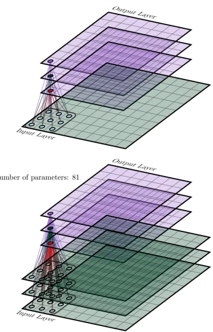
2.10 Top: convolutional layer with one channel in, one channel out. The kernel size is 3×3 and the stride is 1. All output neurons use the same 9 parameters, so there are 9 parameters in total. An output neuron and its receptive field are highlighted left, along with a group of four neurons right, to illustrate the fact that neighbouring neurons can have overlapping receptive fields. Bottom: convolutional layer with three channels in, one channel out. Since convolution kernels span across channels, each output neuron takes input from 27 neurons. Because parameters are shared across spatial axes but not across channels, we need three times as many parameters now, so there are 27 parameters in total. . . . 29

2.11 Top: convolutional layer with one channel in, three channels out. The three output chanels each have their own 9 parameters, so the total number of parameters is 27. Bottom: convolutional layer with 3 channels in, 3 channels out. Each output channel has 27 parameters, so the total number of parameters is 81. Edges of the same colour connect input channel neurons to the same output channel neuron. . . 30

2.12 3×3 convolution with a stride of 2. Since every second position is skipped on both axes, the output will now be 4×4 rather than 8×8. The grey squares represent elements that are computed in stride 1 convolutions but not stride 2 and do not represent actual null values in the output; the three output neurons highlighted are adjacent. Note that the receptive fields of these three neurons span a larger area than if the stride had been 1 (as in Figure2.10, top). . . 32

3.1 a) mouse embryo, an extreme case of overlapping objects consisting of a ball of around 20 cells. b) Human HT29 colon cancer cells, packed very closely. Both images from the Broad Bioimage Benchmark Collection [71]. . . 37

3.2 A sample of detection results on SIMCEP images. Confidence is represented in the transparency of the boxes; all output boxes with confidence above 0.1 are shown. Instead of post-processing with NMS, we simply take boxes with confidence above 0.5 (shown in red) as positive detections. Boxes with confidence below 0.5 are shown in blue. . . 44

4.1 Style augmentation applied to an image from the Office dataset [93] (original in top left). Shape is preserved but the style, including texture, color and contrast are randomized. . . 50

4.2 Diagram of the arbitrary style transfer pipeline of Ghiasi et al. [94]. . . 56

4.3 Output of transformer network with different values for the style interpolation parameterα. . . 58

4.4 Hyperparameter searches on augmentation ratio and style transfer strength (α). Curves are averaged over four experiments; error bars denote one standard devi-ation. Blue lines depict unaugmented baseline accuracy. . . 59

4.5 Comparing test accuracy curves for a standard classification task on the STL-10 dataset [122]. . . 60

4.6 Results of the experiments using the Office dataset. Note the consistent superiority of traditional augmentation techniques combined with style augmentation (red curve). . . 62

4.7 Images from the backpack class, from the Amazon, DSLR and Webcam datasets. The absence of any background in Amazon images makes theDW →Atask more vulnerable to domain bias than AD → W or AW → D, because the Amazon images differ significantly from both DSLR and Webcam images. . . 63

4.8 Examples of input monocular synthetic images post style augmentation. . . 68

4.9 Results of unaugmented model (None), style (Style) traditional (None), and com-plete augmentation (Both) applied to depth estimation on KITTI [96]. . . 69

5.1 Our feature extraction pipeline. We feed our images through a pre-trained VGG16 network, truncated before the fully connected layers, and concatenate the spatial means of three intermediate convolutional layer activations. This yields a vector of multi-scale convolutional features, which we later embed in 2D space via t-sne (see Figure5.6). . . 73

5.2 Receptive field sizes of our chosen convolutional layers, overlaid on a histological image for reference. By pooling from multiple layers, we can extract information about fine texture, individual cells and small clusters of cells. From the outside in, the white squares show the receptive field sizes of convolutional layers 4, 7 and 9 in VGG16. . . 74

5.3 Mean intra-cluster variance as a function of the number of clusters, compared with mean intra-well variance. We cap the number of clusters at 70, as diminishing returns are observed past this point. . . 75

5.4 An assay plate containing 8×12 wells. In an HTS experiment, each well contains a population of cultured cells and a different compound (often repeating the same compound in varying concentrations). In our dataset, images were acquired from four different locations in each well, which means for each compound we have four images that should contain similar looking cells and thus have similar visual embeddings. Source: Wikimedia Commons (CC0 1.0 License). . . 76

5.5 Samples from six of the 70 phenotypic clusters detected by k-means. Each row shows a sample from a different cluster. Rows 2 and 4 show genuine GFP expression. 77

5.6 A t-sne embedding of our dataset, with colours showing phenotypic clusters dis-covered by k-means. For visualization purposes, we set k = 15 here. This interactive data visualization gives scientists a rapid overview of a large dataset, which would be difficult to obtain by sampling individual images. Furthermore, t-sne makes the phenotypic clusters visible in a way that reveals their relationships with one another, and does not enforce a discrete partitioning of the data as clustering algorithms do. . . 80

6.1 A pair of images from our dataset. The left was taken with an iPhone camera, while the right was taken with a Samsung. . . 87

6.2 A pretrained ResNet34 model learns to recognize manufacturers very quickly, and learns to recognize cameras even faster. . . 88

6.3 Test accuracy plot showing the distribution of predicted labels among correct outputs, for a ResNet34 trained on the Disjoint training set, in which all Manu-facturer 1 images are iPhone or Samsung, and all ManuManu-facturer 2 are Huawei or Redmi. For images from iPhone and Samsung cameras the model predicts only Manufacturer 1, while for Huawei and Redmi it predicts only Manufacturer 2, while for the unseen Vivo images it appears to guess randomly, achieving 54% accuracy with a mostly even mix of both classes. Best viewed in color. . . 90

6.4 Test accuracy plot showing the distribution of predicted bottle manufacturers among correct outputs, for a ResNet34 trained on the Partial training set, in which camera type is uncorrelated with class label but only iPhone and Samsung images are present. Overall accuracy across all camera types is close to that achieved when trained on the full dataset, with little bias in favor of familiar camera types. This implies that in the absence of camera / label correlations, the model learns robust features for manufacturer classification, which generalize well to images from unseen cameras. Best viewed in color. . . 91

6.5 Adversarial perturbations applied to two images, classified by a ResNet34 model trained on the Balanced dataset (left) and the Disjoint dataset (right). The left image in each pair shows the input image with the perturbation amplified for visibility and overlaid on top, while the right image shows just the amplified perturbation itself. Strikingly different perturbations to the same image are observed depending on whether the model was trained without camera / label correlations (Balanced) or with them (Disjoint). Best viewed digitally, zoomed in. 92

6.6 A bottle image with local mean thresholding applied, segmenting the batchcode dots. Origin camera classification does not work on such images, indicating that models use something other than the shape and position of the dots to classify cameras. . . 94

6.7 Color jitter augmentations applied to a single image (original in top left). Aug-menting our training images with basic color distortions removes any correlations that may exist between class label and white balance, saturation, hue. . . 95

6.8 Heatmaps representing the camera identification accuracy on 32×32 patches at different locations in single images (white = 100% accuracy, black = 0%). An image from each camera is shown, and the predictions are all from the same ResNet34 checkpoint. The model is able to correctly classify patches from most locations on most images, but some significant dark patches occur. . . 98

6.9 Heatmap representing relative camera classification accuracy of 32×32 crops at different locations in the image, averaged across images from the whole dataset. The lack of bias toward any particular part of the image implies that camera predictive patterns are present uniformly across the images. . . 99

List of Tables

3.1 A specification of our network architecture. Unless otherwise stated, each layer takes the previous layer’s output as input. Nonlinearities are leaky rectified linear [87] with α = 0.1 unless otherwise stated. B is a hyperparameter denoting the number of detectors per “window” (i.e. position in the final feature map,conv7). B= 9 in our experiments. . . 43

3.2 True and false positive rates on training and validation sets. A true positive is counted as any output box with an intersection over union (IoU) above 60% with a ground-truth box, but each ground-truth box can only be paired with a single output box. So if two output boxes cover the same object, then this counts as one true positive and one false positive. Output boxes with less than 60% IoU with any ground-truth box are always false positives. . . 45

4.1 Test accuracies on the Office dataset [93] withA,D andW denoting theAmazon,

DSLRand Webcam domains. DW →Aaccuracies are significantly lower for all methods because the Amazon dataset differs significantly from both DSLR and Webcam, featuring objects superimposed on blank white backgrounds instead of photographed in an office setting. . . 61

4.2 Comparing style augmentation against color jitter (test accuracies on Office, with InceptionV3). These results demonstrate that the textural shifts induced by Style Augmentation provide accuracy gains beyond what can be achieved with simple colour space perturbations. . . 63

4.3 Comparing the results of a monocular depth estimation model [22] trained on synthetic data when tested on real-world images from [96]. . . 64

6.1 Accuracy on the test set when classifying which camera took an image. All architectures tested show high test accuracy, demonstrating that CNNs can easily learn to recognize which camera took an image. The slightly lower accuracies of AlexNet and VGG16 are probably due to these networks requiring input images to be downsampled to 224×224, whereas the other networks can process arbitrary input sizes and so consume the full 1024×1024 images. . . 88

6.2 Manufacturer classification test set accuracy of five models with different training setups. . . 89

6.3 Manufacturer and camera classification accuracy on the test set when trained (and tested) on binary segmented images (see Figure6.6). . . 95

6.4 Manufacturer and camera classification test set accuracy when trained on images with randomized hue, saturation, contrast and brightness. Robust camera classi-fication accuracy implies that image color statistics are not necessary for camera inference. . . 96

6.5 Camera classification test accuracy when trained only on random 32×32 crops of the input data. High accuracy in this regime implies that high frequency features are sufficient for camera classification, and lens deformation (which would not be detectable in a 32×32 region) is not necessary. . . 97

6.6 Camera classification accuracy on right halves of images after training on the left halves. Strong generalization to an unseen area of the training images implies that PNU noise fingerprints of the sort discussed by Lukas et al. [152] are unlikely to be the mechanism by which CNNs are recognizing cameras, because the noise fingerprint on the right side of the images will be different to that on the left side. 97

Chapter 1

Introduction

Deep Convolutional Neural Networks (CNN) trained by gradient descent have revolutionised computer vision in recent years [11]. For the first time ever, the methods of machine vision have become reliable and powerful enough that they now see widespread and profitable deployment in industry. The last five years have seen an explosion in machine learning investment, industrial and scientific applications, hardware, startups, and education. Tasks that require the interpretation of raw images, such as object classification [12], object localisation [13], object counting [14], image segmentation [15], and monocular depth estimation [16], are all now dominated by neural networks.

These machine learning approaches have discarded many decades of hand-crafted vision al-gorithms in favour of end-to-end learning, where every step of processing from raw pixels to final output is learned from experience. CNNs use multiple layers of non-linear processing to incrementally transform a raw image into a prediction, where the action of each layer is determined by learned parameters. For each training example, consisting of an input and a correct output, a scalar error value called the loss is computed, reflecting the difference between the predicted and correct answers. This loss is then differentiated with respect to each parameter in each layer, which allows us to nudge the parameters in a direction that will, on average, result in a lower loss next time the same input is encountered. This approach, in combination with huge training datasets and high performance parallel compute hardware, is what has enabled the deep learning revolution [17].

This rapid growth has been driven in part by the emergence of large scale publicly available benchmark datasets [18], the most famous being the ImageNet dataset for image classification [19]. As of January 2020, ImageNet contains over 14 million images, each annotated with a class label for use as a training example. These enormous datasets not only supply the data needed to train deep neural networks, they also serve as a proving ground for new techniques. The winners of annual competitions such as the ImageNet Large Scale Visual Recognition Challenge (ILSVRC) and Pascal Visual Object Classes (Pascal VOC) become recognized as state of the art approaches, and are quickly adopted as the workhorses of computer vision. This approach has served the research community well, providing a focal point where researchers can compare the empirical performance of competing methods on the fundamental problems of computer vision. However, despite remarkable progress having been made in these benchmark tasks, many obstacles still stand in the way of the application of neural networks to real world problems. Overcoming these obstacles is necessary if efforts of machine learning researchers are to translate into meaningful economic impact and improvements in society.

In this thesis, we describe four contributions that pertain to the practical use of convolutional neural networks, which are briefly outlined in the remainder of this introduction. Chapter 2

provides an introduction to neural networks, deep learning and CNNs which is prerequisite for understanding the rest of this thesis. Chapters 3-6 then describe my contributions in detail, followed by concluding remarks in Chapter7.

1.1

Avoiding Overdetection: Towards Combined Object

Detection and Counting

My first contribution pertains to object detection and counting. Object detection is the task of labeling each object in an image with a bounding box and (typically) a class label. An intuitive and easily implementable approach to object counting is to rely on object detection, first using an off-the-shelf detection network to label all the objects in an image and then counting the number of labels. Most deep learning approaches to object detection result in a fixed number of object bounding boxes being produced, regardless of the number of objects in the image. A confidence value is also predicted for each box, representing the network’s confidence that the box in fact contains an object. By design, the fixed number of boxes is normally greater than the number of objects present, which results in a surplus of boxes being emitted for each object in the image. The excess boxes are normally then pruned by non-maximum suppression (NMS) [20], an

Figure 1.1: Real life contains numerous instances where objects overlap, and yet the non-max suppression algorithm for removing excess detection bounding boxes assumes that strongly overlapping boxes are over-detections of the same object. The two boxes in this example have an intersection-over-union measure of 0.72, which is above the commonly used threshold of 0.7, so one of them would be removed by NMS, even though in this case they are labelling two distinct objects.

iterative algorithm in which boxes which overlap sufficiently with a box of higher confidence are removed. In the majority of cases, this results in one bounding box per object, and so the number of boxes can function as an object count (e.g. [21]). However, in cases where objects are densely clustered or overlapping, NMS may wrongly remove the overlapping boxes (see Figure1.1). A method which only emits one box per object in the first place would clearly solve this problem and obviate NMS in the process, resulting in a more elegant solution. Explaining why most object detection networks share this weakness is also an interesting research question in itself. My contribution here is an answer to that question, and a novel loss function that trains detection networks to emit one box per object.

1.2

Style Augmentation

Domain bias is a common issue in which a model which attains good performance on inputs similar to those it was trained on fails to perform well on dissimilar inputs. In other words, the model is biased towards the domain in which it was trained. To some extent this is expected, but in the case of computer vision, the differences required to cause domain bias issues can be surprisingly subtle. For example, a model trained on images from a video game can perform poorly on images from the real world, even when the virtual world is highly realistic [22]. Meanwhile, research by Tobin et al. [23] shows that CNNs can generalize from very unrealistic virtual worlds to the real world, if the textures in the virtual world are randomized. This suggests

Content Image

Style Image

Restyled Image

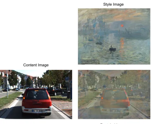
Figure 1.2: The style of Monet transferred to an image from the KITTI dataset. By applying random styles to training images while preserving the labels, we can train networks to be more robust to shifts in texture.

that CNNs are sensitive to texture, and that the key to training a robust model is diversity of texture in the training dataset.

With this in mind, we wondered if it would be possible to improve model robustness by ran-domizing textures in training images as a post-processing step, without access to the rendering engine that created them. Such a method could randomize textures in ordinary photographic images, potentially increasing the robustness of models trained on any image dataset.

Neural style transfer [24] is a deep learning technique for transferring the artistic style of one image to another, allowing one to apply the style of Monet to a photograph, for example. In practice, the concept of artistic style as it pertains to neural style transfer is very similar to the concept of texture [25]. Style transfer alters the distribution of low-level visual features while

preserving the shape of objects. Therefore, if style transfer could be applied to an image in a randomized manner, rather than copying the style of one image onto another, then we might expect a network trained on such images to rely more heavily on shape than on texture for its judgements. This would encourage good generalization across domains, since a model that can remain accurate when texture is randomized can probably remain accurate when processing slightly different images from another domain.

The practice of randomly pre-processing training images with transforms that do not render the image unidentifiable is called data augmentation, and has been in use since the early days of learned vision (e.g. [26, 27]). It is seen as a way to artificially inflate a small training dataset (e.g. in [28]), and can also be thought of as a way to train a network to be invariant to a certain transform. For example, random horizontal flipping is a common image augmentation because we know that mirroring an image should not affect its label, and Simard et al. [27] inject elastic deformations into handwritten digit images to mimic the distortions caused by the uncontrolled oscillations of human hand muscles. Since the technique discussed in this chapter is also applying randomized label preserving transforms to training images with the intent of teaching invariance to said transforms, it too belongs under the umbrella of data augmentation, hence the name “Style Augmentation”. Style Augmentation is designed as a generic data augmentation technique, which could be easily slotted into any machine learning vision process.

1.3

Phenotypic Profiling of Chemical Clusters with

Gen-eric Deep Convolutional Features

Out of all the obstacles to deep learning’s practical deployment, its dependency on large quantities of labelled training data is probably the most common. With a few notable exceptions (such as GPT-2 [29]), the state-of-the-art results in most deep learning benchmark tasks have been achieved via supervised learning, in which the target output for each training example is produced manually by a human (e.g. [12, 13, 15]). The ImageNet dataset / ILSVRC challenge is the most prominent example of supervised learning; each of the 14 million images in ImageNet was manually annotated with a class label via the Amazon Mechanical Turk crowdsourcing platform [30]. This is an enormous and expensive undertaking, which most organizations do not have the resources to reproduce for their individual problems.

The contribution in this chapter concerns a project in collaboration with AstraZeneca, in which a large, unlabelled image dataset had to be split into classes. AstraZeneca are a pharmaceutical

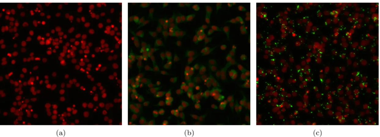
firm who use high throughput screening (HTS) techniques for novel drug discovery. HTS uses robotic systems to test interactions between large numbers of novel compounds (typically in the millions) and biological cells in parallel, with the aim of winnowing a field of millions of compounds down to a few promising leads, known as “hits”, which will then proceed to further test, preclinical studies, and finally clinical trials. In this case, a set of compounds were applied to human kidney cells and imaged with a wide field fluorescence microscope after an incubation period. These cells were genetically engineered to express both Green Fluorescent Protein bound to Low Density Lipoprotein Receptor (LDLR-GFP), and Induced Degrader Of LDLR (IDOL). Since IDOL breaks down the LDLR-GFP complex, its presence causes the absence of green fluorescence, and anything that inhibits IDOL results in the presence of green fluorescence. The aim of the project was to discover compounds that inhibit IDOL. However, presence of green fluorescence alone is not sufficient - it also matters where within the cell that green signal is localised (e.g. within the cytosol, within the membrane, within the golgi apparatus). The visual manifestations of these differences are complex and highly variable (see Figure 1.3), which makes it difficult to detect them using traditional image processing techniques. The inevitable occurrence of artefacts during image acquisition complicates matters further. Due to the lack of a positive control, the researchers also did not have a clear idea of what a genuine hit looked like; this shifted the emphasis away from binary hit/non-hit classification and towards dataset exploration and class discovery. In a supervised learning project, the network learns from manually generated annotations that explicitly label the category of each image. Is it possible for a CNN to classify the images in this domain specific dataset even though no such labels are available to learn from?

In this chapter we present a pre-clinical screening workflow that exploits a pre-trained CNN to cluster a large cellular image dataset by visual similarity, producing a small number of phenotypic clusters that a domain expert can quickly assess. Grouping similar images together allows biologists to apply their judgement to entire clusters of images at once, rather than assessing images one by one, resulting in much faster pre-clinical screening. ImageNet pre-trained CNNs are known to detect a broad range of low level features [31], and it turns out that these are rich enough to produce distinct responses for cellular images of different phenotypes, even though the network itself was trained to classify images of a very different nature. By passing cellular images through the CNN, feature vectors for the images can be derived from its internal dynamics. These are then grouped by an unsupervised clustering algorithm, and represented graphically via a t-SNE plot, providing an overview of the dataset in which different phenotypes emerge as distinct clusters of points.

(a) (b) (c)

Figure 1.3: Three samples from the high throughput imaging dataset. a) no IDOL inhibition, hence no LDLR-GFP is present, only the cellular nuclei, stained red with Hoechst stain, are visible. b) LDLR-GFP visible as green fluorescence in the cytoplasm c) LDLR-GFP, localised within cellular organelles, visible as bright green dots.

1.4

Camera Bias In Fine Grained Classification: Effects

and Mitigations

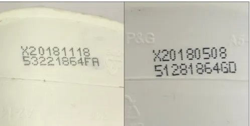
CNNs (and machine learning methods in general) will exploit any patterns in their training data to minimize their loss functions. When we show a model an input / output training example, we are telling it what the correct output is for that input but not why that output is correct. The rules for mapping input to output have to be inferred from many such examples, and the model has no way of knowing if a rule that minimizes loss over the training set will not generalize to the test set. Sometimes this leads to unwanted behaviour, particularly if the model learns to exploit a some subtle idiosyncrasy in the training data, which the engineer may not be aware of. In this chapter, we investigate an unusual form of domain bias that interfered with another industrial collaboration, this time with Proctor & Gamble. This project aimed to apply standard CNNs with supervised learning to detect counterfeit shampoo bottles, by observing subtle differences in the batch code printed on the underside of the bottle. In this chapter, we prove that correlations between the class label (real or counterfeit) and the type of camera that captured the image are exploited by CNNs, resulting in a model that “cheats” by inferring the class from the camera type. Such models are unable to generalize to domains where the class label does not correlate with camera type. We also perform experiments to determine how CNNs are able to recognize cameras from the images they produce, since the differences between images from

Figure 1.4: Batch codes from a genuine and counterfeit shampoo bottle (left, right). Human domain experts achieve around 60% accuracy on this classification task. With extremely fine-grained classification problems like this, it is often very unclear which features a CNN is exploiting when it achieves high classification accuracy. Answering this question would be useful both for validating the trustworthiness of the model, and for understanding the differences between real and counterfeit bottles.

Chapter 2

Deep Neural Networks for

Computer Vision

Deep neural networks (DNN), once a fringe sub-field considered by most to be unworkable, exper-ienced a sudden and spectacular rise to prominence in 2012 when a DNN achieved breakthrough performance in the ImageNet Large Scale Visual Recognition Challenge (ILSVRC) [32]. Alex Krizhevsky’s winning entry, which became known as AlexNet, improved on the previous year’s classification accuracy by an unprecedented 15% margin [19], establishing DNNs as the dominant technique in computer vision and provoking a massive resurgence of interest in neural networks generally. Since then, DNNs have come to dominate in a number of fields besides computer vision, most notably reinforcement learning [33] and natural language processing [34].

In this chapter, we will provide an introduction to neural networks, their history, key break-throughs, their structure and the methods by which they are trained. In particular we will focus on convolutional neural networks (CNN), which have become the workhorse of modern computer vision.

2.1

Neural Networks

Artificial neural networks are a biologically inspired model of computation, first proposed by McCulloch and Pitts in 1943 [35]. This paper developed the first model of an artificial neuron

x

x

x

x

Σ

W

W

W

W

y

Inputs

Weights

Weighted sum,

threshold function

Output

Figure 2.1: A McCulloch and Pitts artificial neuron. It computes a single output value from multiple inputs. If a weighted sum of the inputs exceeds the neuron’s threshold value, then the output is 1, otherwise it is 0.

(commonly referred to now as a McCulloch-Pitts (MP) neuron), and analyzed their computa-tional properties.

MP neurons are very simple. Like biological neurons, each MP neuron receives input from several other neurons, and can emit a single output value when sufficiently excited by its inputs. They have weights on their incoming connections, which determine whether those input signals are excitatory or inhibitory; the neuron fires if and only if the weighted sum of its inputs exceeds some threshold value (see Figure 2.1). A neuron that fires is said to be activated, and its output value is often referred to as its activation. It was shown that, despite their enormous simplifications compared to real neurons, networks of MP neurons could implement elementary logic gates such as AND, OR and NOT. This means that networks of artificial neurons are able to represent arbitrary propositional logic formulas. Not only that, but neural networks whose directed connections form cycles are computationally universal, i.e. able to represent any program. Although this model has been tweaked many times since 1943, the basic principles of neural networks were laid down in this seminal work:

• Neurons are discrete computational units with directed, weighted connections between them

• Neurons receive input signals from other neurons, and send output signals to other neurons, according to the connections between them

• Neurons compute weighted sums of their input signals, and their output value is a nonlinear function of this weighted sum

• A neural net contains a subset of neurons called input neurons, who receive no input from other neurons and whose output values are raw input observations

• A neural net contains a subset of neurons called output neurons, who do receive input from other neurons and whose output values form the output of the neural net.

McCulloch-Pitts neurons are very limited. The connection weights are constrained to be either +1 or−1, the output of each neuron is either 0 or 1, and most importantly, there is no learning algorithm. Despite their theoretical universality, there was no general algorithm for determining the connections and weights needed to implement a given function or solve a given task. They are also clearly quite ill-suited to representing real valued functions.

As computers became more powerful in the decades that followed, many researchers advanced the study of neural networks in different directions. Among them was Frank Rosenblatt, who in 1958 published the perceptron [36], a simple neural machine originally applied to image recognition. A perceptron has a layer of input neurons, and a layer of output neurons. A perceptron neuron computes a weighted sum of its real valued inputs, using real valued weights, and then passes that weighted sum through a non-linear function to compute its output value. This output is often referred to as the neuron’s “activation”, and the non-linear function as an “activation function”. If we treat the input layer values as a vector~x, and the corresponding weights as another weight vectorw~, then a perceptron neuron can be said to perform the following computation:

y=f(~x·w~+b) (2.1)

where f is a continuous activation function in place of the threshold function in MP neurons, and b is a constant bias term. When we have more than one neuron dependent on the same

set of inputs (for example, the “hidden layer” in Figure2.2), we can treat their activations as a single vector~y, the connection weights between the two layers as a matrixW, and the biases as a vector~band describe the action of the entire layer as follows:

~

y=fW~x+~b (2.2)

where the activation functionf is now implicitly applied elementwise across the vector of pre-activation values (also known aslogits). When f is a threshold function (as in MP neurons), or a continuous version of it such as the logistic function, a perceptron neuron can be understood as a linear classifier - that is, it classifies input vectors based on which side of a hyperplane they lie on. The weight vector is the normal vector of this hyperplane, and the bias determines its distance to the origin.

Input Layer

Hidden Layer

Output Layer

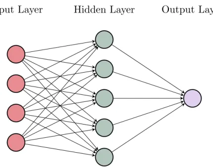
Figure 2.2: A multi-layer perceptron has two (or more) layers of modifiable connections. Even with only one hidden layer, an MLP is theoretically able to approximate any function from the input to output domain to arbitrary accuracy, given sufficient neurons in the hidden layer.

The single layer perceptrons described above are only capable of learning linearly separable patterns, as famously highlighted by Marvin Minsky and Seymour Papert in their 1969 book

Perceptrons [37]. This relatively trivial observation has been the source of much controversy between connectionist and symbolic AI for several decades [38, 39]. The linear separability limitation can be overcome by inserting an additional “hidden layer” between the input and output layers, creating a multi-layer perceptron (MLP, see Figure2.2).

MLPs are universal function approximators: with enough neurons in the hidden layer, they are capable of approximating arbitrary functions between finite dimensional vector spaces with arbitrary accuracy [40, 41]. The exact shape of this function depends on the values of the network’s inter-neuron connection weights and neuron biases. The architecture of the network (number of layers, number of neurons in each layer, connectivity between layers) therefore defines not one function but a set of functions, parameterized by these weights and biases (which indeed are together referred to as network parameters). To implement a function that does something useful, one must find good values for these parameters.

Unfortunately, manually specifying good values for weights and biases is something human programmers are extremely bad at. The 20th century saw many attempts to address this difficulty using machine learning, including both supervised learning approaches such as the delta rule [42], and biologically inspired unsupervised approaches such as Hebbian learning [43], self-organizing Kohonen maps [44] and Hopfield networks [45]. Eventually, backpropagation of errors emerged as the dominant technique for training neural networks (for a more thorough account see Jurgen Schmidhuber’s analysis [46]).

The idea is to make incremental updates to the weights and biases (henceforth referred to as parameters) which, on average, improve the performance of the network at a given task. This requires two things: a precise, quantitative metric of “performance for a given task”, and some way of estimating the optimal direction in which to nudge the parameters to increase that performance metric. The former is provided by something called a loss function, and the latter is provided by backpropagation.

2.2

Loss Functions

A loss function is an error function to be minimized, whose formula defines the task to be learnt by the network. For a supervised classification task (e.g. image recognition), this function is nearly always cross entropy, defined as such:

H(p, q) =−

n X

i=1

p(ci)log(q(ci)) (2.3)

Cross entropy is a quasi distance metric between the two probability distributionspandq(quasi becauseH(p, q)6=H(q, p)). In our case, theciare possible class labels,nis the number of classes,

pis the true probability distribution for a given sample (which we know because the images are pre-annotated), and q is the network’s predicted probability distribution. This requires us to interpret the output of our network as a probability distribution, to which end we apply the softmax activation function:

y=q(ci) = softmax(z)i=

ezi

Pn

j=1ezj

(2.4)

where y is the network’s final (post-activation) output and z is the vector of pre-activation logits of the network’s output layer, which should contain one neuron per class. Softmax is an unusual activation function in that it is not elementwise: the activation of each unit in the vector depends on the logits of all the others due to the summation in the denominator. This summation normalizes the activations so that they sum to one, as a probability distribution must - an increase in the activation of one neuron will therefore result in a decrease in the activations of the others. Interpreting the output of a neural network as a probability distribution over possible class labels is a key component in training neural networks for discrete classification tasks, as it allows us to define a continuous loss function in which small changes to the real valued output vector produce a non-zero change in the loss. In mathematical terms this means we can define adifferentiable

loss function, which would not be the case if the loss were a function of, say, argmax(z) (because the argmax function is discontinuous and therefore non-differentiable, changing all at once only when the highest value logit is overtaken by another).

Our true probability distribution,p, is likewise denoted by a one-hot vector:

p(ci) =    1 if i = t 0 otherwise (2.5)

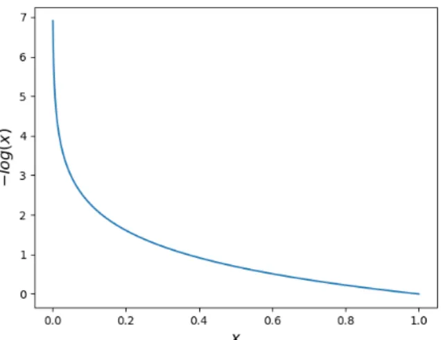
Figure 2.3: Cross entropy loss as a function of the predicted probability of the correct class (x= softmax(yt)). The steep gradient as xapproaches 0 compensates for the low gradient of

the softmax with respect toytwhen softmax(yt) is low.

where ctis the target or true class label. With this in mind, it can be seen that Equation 2.3

simplifies to the predicted negative log likelihood of the correct class:

H(p, q) =−log(q(ct)) =−log(yct) (2.6)

Thus, softmax output defines a continuous output space for a discrete classification problem, and cross entropy loss defines a continuous “wrongness” metric over these outputs - at least for a given instance of the problem. Of course, a correct answer for one particular input does not imply that the network has learned anything useful; to prove that the network has mastered a task, we must achieve correct answers on many diverse instances. Therefore, our true loss function for a classification task is theaverage cross entropy over a large dataset of training examples:

L(X, θ) = 1

|X|

X

(x,t)∈X

−log(f(x;θ)t) (2.7)

Where X is a set of training examples, each consisting of an input xand a class label t, and f(x;θ) is the network’s softmax output, given inputxand current parametersθ.

2.3

Backpropagation

Backpropagation is not a neural network specific technique, nor is it a complete learning algorithm per se. Backpropagation is an algorithm for automatically differentiating a composite function through repeated application of the chain rule of differential calculus. The chain rule states that the derivative of the composite of two functionsf and g is the product of the derivatives of f andg:

(f(g(x)))0 =f0(g(x))·g0(x) (2.8)

or, in Leibniz notation:

dz dx = dz dy · dy dx (2.9)

wherezis a function ofy, which is a function ofx. By induction, the chain rule can be extended to function compositions of arbitrary length:

d dxf1(f2(f3(. . . fn(x)))) = df1 df2 ·df2 df3 ·df3 df4 . . .dfn dx (2.10)

Since the activation of each layer of a neural network is a function of the previous layer, neural networks are composite functions. To make this clearer, consider the following computational graph, representing the three layer perceptron shown in Figure2.2.

The edges represent computational dependencies between the various input, output and inter-mediate values, which are represented as nodes in the graph. The value of a node can only be computed given knowledge of the values of its parent nodes. “Running” a neural network - that is, computing its output y starting from only its input x and parameters wi, is a process of

continually computing the values for nodes whose dependencies are known, until we reach the output node. In deep learning parlance this is known as aforward pass, since it follows the edges of the computational graph forward from input to output. Backpropagation, in contrast, is often referred to as abackward pass, since it begins at the loss and follows the edges backward to the parameter nodes. In much the same way that the forward pass can only compute the values of

x

z

w

a

z

w

a

z

w

y

L

c

Figure 2.4: A computational graph for the network depicted in Figure 2.2. Nodes denote the input vector x, output vectory, intermediate values zi, ai, weights and biases (wi), class label

ctand loss L; edges denote computational dependencies. zi denote pre-activation logits, ai are

activations. Leaf nodesxandwiare nodes whose values are known a priori, everything else must

be computed from the values of its parent nodes. Backpropagation begins at the loss (green) and works backwards, terminating at the parameter nodes (red).

nodes whose parents’ values are known, the backward pass can only immediately compute the gradient of a node whose child’s gradient is known∗.

Once backpropagation has computed the gradients of all the network’s parameters, we are ready to update those parameters. If we think of the concatenation of all weights and biases as a single vector of parametersθ, then backpropagation yields us∇θL(x, θ), the gradient vector of the loss

(for the given input x) with respect to the parameters θ. This vector points in the direction of the steepest rate of increase of loss in parameter space; since we wish to decrease the loss, we therefore take a small step in the opposite direction. So long as this step is small enough that the gradient does not change too much over the distance travelled, this will result in a new parameter vector θ0 such thatL(x, θ0)< L(x, θ).

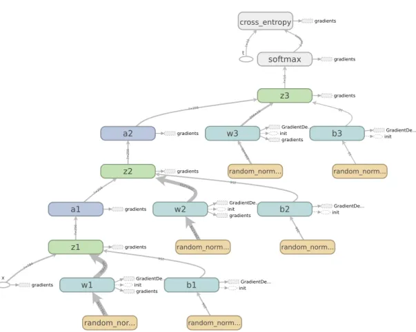
Computational graphs are not just an intuitive and elegant way to visualize a neural network; most modern neural network libraries use computational graphs explicitly to represent neural networks. In TensorFlow [47] for example, a typical program begins by constructing a computa-tional graph representing the desired neural net, which can later to visualized in a web browser (see Figure2.5).

2.4

Stochastic Gradient Descent

With a well defined objective function and a method for computing its gradient for each of our parameters, neural network training reduces to an optimization problem, which we can solve

∗_{To avoid confusion, it should be mentioned that the “gradient of nodei” refers to the gradient of the losswith}

respect toto nodei. Although backpropagation can in principle compute the gradient of any node with respect to any upstream node, there is rarely any reason to differentiate anything other than the loss.

784×256 256×256 256×10 256 256 10 ?×78 4 784× 2 5 6 25 6 ?×256 ?×25 6 25 6× 25 6 6 25 ?×256 ?×256 256× 10 10 ?×10 ?× 10 3 te ns or s gradients x t random_nor... GradientDe... init gradients w1 random_norm... GradientDe... init gradients w2 random_norm... GradientDe... init gradients w3 random_norm... GradientDe... init b1 random_norm... GradientDe... init b2 random_norm... GradientDe... init b3 gradients z1 gradients a1 gradients z2 gradients a2 gradients z3 gradients softmax gradients cross_entropy

Figure 2.5: A TensorFlow computational graph corresponding to the one in Figure 2.4. Leaf nodes (small white ellipses) are points at which training data is fed into the graph. One isx, the image, while the other ist, the class label, used in the cross entropy loss (which is included in this diagram but not in Figure2.4). Parameter nodes show a computational dependency on random normal distributions - this is because weights and biases are generally initialized by sampling from normal distributions.

with first-order gradient descent. Gradient descent is a simple, intuitive, well studied technique for finding local minima of scalar functions. Consider a differentiable function F : Rn → R. Gradient descent allows us to begin at an arbitrary point θ0 ∈Rn, and iteratively update this point by shifting it a small amount in the opposite direction to the gradient of F. This results in a series of points that converges on a local minimum, at which the gradient is zero. Formally,

θt+1=θt−α∇θF(θt). (2.11)

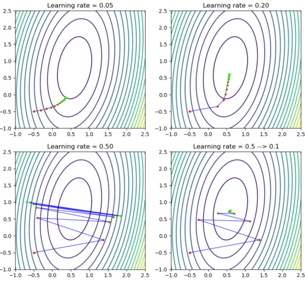
In the context of machine learning, α is called the learning rate, and is generally the most important hyperparameter in any deep learning task. If it is too large then θt+1 may be larger

thanθtand the sequence may diverge, since∇θF(θt) tells us only the instantaneous gradient at

the point θt. Likewise if αis too small, then the sequence will take too long to converge, since

each gradient descent step requires another expensive gradient evaluation via backpropagation (see Figure2.6).

Recall that the loss function we wish to optimise (Equation 2.7) is actually defined as the mean of the losses of individual samples x ∈ X. So far we’ve only discussed computing and backpropagating the loss for an individual sample, but due to the linearity of expectation, the gradient of the mean loss is just the mean of the gradients of the individual losses:

∇θEx∈X[L(x, θ)] =Ex∈X[∇θL(x, θ)] (2.12)

In practice, the number of training inputs|X| is often very large, particularly in deep learning settings where copious training data has proved to be quite important. Computing Equation2.12

in full can therefore be computationally expensive, which in turn limits the rate at which we can perform parameter updates. This problem can be greatly mitigated by computing Equation2.12

over minibatches rather than over the full dataset. A minibatch is a small batch of random samples fromX, the size of which is generally limited by the amount of memory available. This random sampling, then, is where the stochasticity of stochastic gradient descent comes from. So long as the minibatch is sampled uniformly at random, then the mean gradient over a minibatch is an unbiased estimate of the gradient over the full dataset (Equation 2.12). The variance of this estimate tends towards zero as the minibatch size tends towards |X|, but with diminishing returns. A minibatch much smaller than|X|will typically provide a decent estimate in a fraction of the time required for the full dataset.

Figure 2.6: Ten steps of gradient descent on a quadratic bowl loss function, with different learning rates. With too low a learning rate, ten steps is not enough to reach the local minimum (upper left), whereas with too high a rate the optimizer diverges (lower left). A good strategy is to start with a high learning rate and reduce it throughout training (lower right). This attains the lowest loss of all, without having to guess a good learning rate (upper right).

2.5

Deep Learning

Although 3-layer MLPs are universal function approximators, this theorem says nothing about the efficiency of such a representation. In particular, we desire models that can represent high dimensional functions with many variations using a tractable number of neurons. Not only are smaller networks less computationally demanding; they also have fewer parameters to train, and thus present a smaller search space in which fewer labelled examples are required to locate a good solution. There are several compelling arguments for whydeep neural networks, composed of many layers of neurons, might outperform shallow neural networks in these regards [48], particularly for the archetypal AI problem of computer vision.

A sensible sounding plan for image recognition is to build a hierarchy of increasingly complex and abstract visual patterns, beginning with small local features such as edges and culminating in high-level semantic concepts such as “dog”. A pattern at one level of such a hierarchy might be composed of several patterns detected by the level below. For example, one layer might detect lines, the next may recognize certain arrangements of lines as forming letters, and the next may recognize sequences of letters as forming words. Similar arguments apply to other cognitive tasks such as sentence parsing.

So intuitive is this hierarchical approach, that it appears regularly in much of the state of the art prior to deep learning (e.g. part-based models [49–51]). Breaking a problem down into a series of sub-problems is a very generic problem solving template, which occurs not only in human engineering but also in biology, for example the Golgi apparatus, whose stacked layers sequentially modify proteins, and in the primate visual cortex [52].

Another compelling argument for hierarchies of features is feature reuse. By exploiting the underlying similarities between related tasks (such as the recognition of different object classes), a model can both represent those computations more compactly and learn them more efficiently, requiring less data [48]. For example, an intermediate feature such as a horizontal edge may be used in the detection of multiple higher level features such as object parts, which themselves may each contribute to the detection of multiple whole objects. Even a binary classifier, which detects only a single type of object, should in theory benefit from feature reuse, because the overall task is composed of many related sub-tasks, computed by individual neurons, each of which shares features from the layer before. Feature reuse can also be seen as analogous to

structured programming [53], in which code is written once, and encapsulated in functions that can be called many times. Not only does this result in more compact code, it also means that a

single update to a function can improve performance in all tasks that use it. This all suggests that deep architectures could make more efficient use of neurons (or whatever other computational units are used), compared to shallow architectures such as the three-layer perceptron discussed earlier.

Finally, there are some theoretical results proving that certain types of function can be repres-ented more efficiently by deeper networks of computational elements than by shallower ones. For example, Johan Hastad proved that for allk, there exist k+ 1 depth boolean logic circuits with a linear number of gates with respect to input size, which require an exponential number of gates to simulate with a circuit of depthk [54]. Later, Hastad and Goldmann proved a similar result for networks of MP neurons [55]. Likewise, Bengio et al. [56] argue that a number of toy problems can be solved more efficiently by deep architectures than by shallow ones. More rigorous results are derived in [57], showing that a deep network can model a greater number of piecewise linear regions than a shallow network with the same number of hidden neurons.

Deep learning is often contrasted with classifiers based on hand engineered features, which was the dominant machine learning paradigm prior to deep learning (see [19]). Feature engineering levers expert domain knowledge to construct hard-coded functions of the input, whose values are likely to be immediately relevant to the classification task. The learnable part of such models is typically very small, for example a single layer of neurons with learnable parameters, or a nearest neighbour classifier, whose inputs are the hand crafted feature vectors. In machine vision, a typical example of such hand crafted features is Gabor filters. Deep learning replaces hand crafted features with many layers of learnable nonlinear processing, allowing the network to effectively learn its own features, directly from raw input.

2.5.1

The Vanishing Gradient Problem

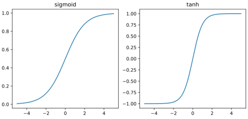
Despite its promising motivations, deep learning failed to yield competitive results on standard benchmarks for many years. Although they were known to be more expressive than shallow networks, deep neural networks proved to be much harder to train. The main reason for this was eventually identified and became known as the vanishing gradient problem, formalized by Sepp Hochreiter in 2001 [58]. The problem is that gradients attenuate exponentially as they propagate through the network during backpropagation, resulting in very small magnitude gradients in the earliest layers of the network, particularly at the beginning of training (see Figure2.8). The main culprit turned out to be the saturating activation functions used at the time, namely sigmoid and

4 2 0 2 4 0.0 0.2 0.4 0.6 0.8 1.0

sigmoid

tanh

Figure 2.7: Sigmoid (a.k.a. logistic function) and tanh (hyperbolic tangent) are saturating nonlinearities, that is, their gradients are close to zero whenever their input is far from zero. This causes gradients to attenuate exponentially through layers of saturating neurons.

tanh. Saturating functions are bounded, which causes their gradient to approach zero as their input tends to infinity (see Figure 2.7). The gradients of these functions are in fact always less than one, and because the chain rule propagates gradients multiplicatively (see Equation 2.10), this means that gradients are multiplied by something less than one at every layer during the backward pass. An intuitive interpretation is that a small change to a weight in the first layer will produce a smaller effect in the activation of its neuron, which in turn will produce still smaller changes in its own downstream neurons, resulting in a vanishingly small effect on the network’s output. It is therefore necessary to use non-saturating activation functions, the de facto standard now being rectified linear function (ReLU(x) = max(0, x)). By mitigating the vanishing gradient problem, ReLU activation can be considered one of the key enabling technologies in deep learning [17].

2.6

Convolutional Neural Networks

The quest for computer vision has been pursued since long before we had any idea how difficult it would be. We wish to build machines that can perform all the same functions as the human visual system; such a task could alternatively be described as “inverse computer graphics”, that is, inferring properties of a 3D world from a 2D projection of it. Vision comprises a broad set of

0

2000

4000

6000

8000

Iteration

0.000

0.005

0.010

0.015

0.020

0.025

Gradient magnitude

Gradient magnitudes with sigmoid activation

Layer 1

Layer 2

Layer 3

0

2000

4000

6000

8000

Iteration

0.01

0.02

0.03

0.04

0.05

0.06

0.07

0.08

Gradient magnitude

Gradient magnitudes with relu activation

Layer 1

Layer 2

Layer 3

Figure 2.8: Top: Gradient magnitudes of bias vectors for the three hidden layers of a multi-layer perceptron, trained on MNIST (layers numbered from first to last in legend). Because of the saturating sigmoid non-linearity, earlier layers have smaller gradients than deeper layers, with first layer gradients close to zero at the beginning of training (as reported in [59]). Bottom: As above, but with recitified linear activation in place of sigmoid. First layer no longer suffers from vanishing gradients.

overlapping computational tasks, including object recognition, depth perception, estimation of 3D shape, tracking of moving objects, orientation of oneself in a 3D environment, handwritten text recognition, and inferring the properties of unrecognized objects by extrapolation from similar examples. All of this must be done in the presence of sensor noise, inconsistent lighting and shadows, partial occlusion of objects, and distraction by irrelevant stimuli. Prior to 2012, state of the art vision models generally approached this problem by extracting hand engineered feature vectors which were classified using a simple machine learning model. For example, the 2010 and 2011 winners of the ILSVRC image recognition challenge were both hand crafted feature extraction pipelines followed by support vector machines [19]. As discussed in the previous section, hand engineered features are often task-specific and require expert domain knowledge. More importantly, their effectiveness for image classification appears limited, such solutions often proving too brittle to see much real world deployment. If we are unable to hand craft suitable features for vision then it is natural to try ceding this task to machine learning; perhaps a deep neural network could discover more generalizable features by brute gradient descent? Learning machine vision directly from raw pixels poses certain challenges which are absent from simpler machine learning tasks:

• Complexity of task- vision tasks typically have very high intra-