Improving bank erosion modelling at catchment scale by incorporating 1
temporal and spatial variability 2
V.J. Janes1,2, I.Holman1*, S.J. Birkinshaw3, G.O’Donnell3, C.G. Kilsby3. 3
1
Cranfield Water Science Institute, Cranfield University, Bedford, MK43 0AL, UK. 4
2
Lancaster Environment Centre, Lancaster University, LA1 4YQ, UK. 5
3
School of Civil Engineering and Geosciences, Newcastle University, Newcastle, 6
NE1 7RU, UK. 7
*Corresponding author: Tel. +44 (0)1234 758277, Email: [email protected] 8
9
Abstract 10
Bank erosion can contribute a significant portion of the sediment budget within 11
temperate catchments, yet few catchment scale models include an explicit 12
representation of bank erosion processes. Furthermore, representation is often 13
simplistic resulting in an inability to capture realistic spatial and temporal variability in 14
simulated bank erosion. In this study, the sediment component of the catchment 15
scale model SHETRAN is developed to incorporate key factors influencing the 16
spatio-temporal rate of bank erosion, due to the effects of channel sinuosity and 17
channel bank vegetation. The model is applied to the Eden catchment, north-west 18
England, and validated using data derived from a GIS methodology. The developed 19
model simulates magnitudes of total catchment annual bank erosion (617 - 4063 t yr -20
1
) within the range of observed values (211 - 4426 t yr-1). Additionally the model 21
provides both greater inter-annual and spatial variability of bank eroded sediment 22
generation when compared with the basic model, and indicates a potential 61% 23
increase of bank eroded sediment as a result of temporal flood clustering. The 24
hydrologic models and has general applicability to temperate catchments, yet further 26
development of model representation of bank erosion processes is required. 27
28
Keywords 29
Bank erosion, sediment, sinuosity, vegetation, catchment. 30
31
Introduction 32
Sediment erosion and transport are natural geomorphic processes within river 33
catchments, but high magnitude events and anthropogenic influences (such as 34
deforestation and over-grazing) can easily disrupt the sensitive equilibrium between 35
them. When these changes result in increased sediment loads, they may have 36
numerous detrimental effects to the river system; increased sedimentation in 37
channels and floodplains affecting land-use and changes in river morphology and 38
behaviour (Owens et al, 2005), flooding (Mcintyre et al, 2012), and disruption to 39
habitats and decreased biodiversity (e.g. salmonid spawning, Soulsby et al, 2001). 40
Furthermore, as sediments act as a transport vector for pollutants such as heavy 41
metals, increased sediment delivery may also change the chemical composition of 42
the river resulting in negative impacts to the ecosystem (eutrophication, Owens and 43
Walling, 2002; and toxicity effects, Mackin et al, 2003). Consequently, information 44
on sediment generation and transport through river systems at a catchment scale, 45
and their temporal and spatial variability is increasingly important to support 46
catchment management. 47
Sediment fingerprinting techniques have been applied to a number of catchments 48
worldwide to understand the relative importance of different sources of sediment, 49
significantly to catchment sediment budgets, in some cases representing up to 48% 51
of total sediment supply (Walling, 2005; Walling et al, 2008). Furthermore, where 52
channel banks contain contaminated sediments the contribution of bank erosion to 53
pollutant supply has also been noted to be significant; for example, lead supply from 54
banks of 9 kg m-1 yr-1 (Glengonnar Water, Scotland UK, Rowan et al, 1995) and 55
mercury supply of 2.7 kg km-1 yr-1 (South River, Virginia USA, Rhoades et al, 2009). 56
The severity of bank erosion is influenced by numerous factors such as the 57
presence of bank vegetation (through both mechanical and hydrological factors) 58
(Micheli and Kirchner, 2002; Bartley et al, 2008; Simon and Collison, 2002); 59
discharge and flow regime (Julian and Torres, 2006; Hooke, 2008; Surian and Mao, 60
2009); lithology (Hooke, 1980); channel confinement (Lewin and Brindle, 1977; 61
Janes et al, 2017); and anthropogenic influences (Winterbottom and Gilvear, 2000; 62
Michalková et al 2011). As such rates of channel bank erosion are both highly 63
temporally and spatially variable (Hooke, 1980; Bull, 1997; Lawler et al, 1999; 64
Couper et al, 2002). 65
Management of sediment and other diffuse pollution issues at a catchment scale 66
is imperative due to the connectivity of the system. Models provide a valuable means 67
of estimating sediment generation and transport at catchment scales, potentially 68
providing insights into the spatio-temporal generation and transport of sediment and 69
the system responses to longer term changes such as climate change. However, 70
many existing catchment-scale hydrological and water quality models contain no 71
explicit representation of channel bank erosion processes; CREAMS - Chemicals, 72
Runoff and Erosion from Agricultural Management Systems (Knisel, 1980), 73
ANSWERS - Areal Nonpoint Source Watershed Environment Simulation (Beasley 74
1990), SWAT – Soil and Water Assessment Tool (Arnold et al, 1998), and PSYCHIC 76
– Phosphorus and Sediment Yield Characterisation In Catchments (Davison et al, 77
2008). Additionally, those models which do contain representations of bank erosion 78
only account for few of the numerous aforementioned factors controlling channel 79
bank erosion rates which limits their ability to simulate the observed spatial and 80
temporal variation of sediment generation through bank erosion processes. For 81
example, the semi-distributed INCA-Sed model (Jarritt and Lawrence, 2007) 82
accounts for bank eroded sediment within in-stream sediment sources using a power 83
law relationship incorporating discharge and calibration parameters. As 84
acknowledged by the authors, a range of sub-reach scale processes are not 85
included within the model and therefore only a broad range of seasonal trends can 86
be observed, rather than finer temporal and spatial variation. The model SedNet 87
provides a mean-annual sediment budget (Prosser et al, 2001; Wilkinson et al, 88
2009). Riverbank erosion within the model is based on an empirical relationship 89
related to stream power, the extent of channel bank vegetation, and non-erodible 90
surfaces. Whilst this method incorporates some factors influencing the spatial 91
variation of bank erosion rates and provides an estimate of annual sediment 92
generation, it does not account for finer-scale temporal variability or provide an 93
indication of event-based bank erosion. Whilst a dynamic version of the model (D-94
SedNet, Wilkinson et al, 2014) exists, this model disaggregates longer term data to 95
provide daily output this model, meaning the model is unable to fully capture the 96
temporal variability observed in sediment loads. 97
Detailed numerical models of bank erosion have been shown to simulate channel 98
migration with reasonable accuracy (Darby et al, 2002, 2007; Duan 2005; Nagata et 99
bank properties, shear stresses acting on channel banks and subsequent erosion. 101
However these models lack simulation of catchment hydrology, and the high-102
resolution data required for such models and their computational requirements limit 103
their application to reach scales. Therefore to provide estimates of bank-eroded 104
sediment at a catchment scale, alternative methods are required. 105
If models are to provide the more holistic representation of sediment processes at 106
a scale that is needed to inform catchment management, further research is needed 107
to improve two key aspects of catchment models; continuous simulation of coupled 108
hydrological and sediment processes, and the ability to replicate both temporal and 109
spatial variability of natural systems. This paper therefore describes the further 110
development and application of the Système Hydrologique Européen TRANsport 111
(SHETRAN) model (Ewen et al, 2000) to provide improved spatio-temporal 112
representation of channel bank erosion processes within simulated catchment 113
sediment budgets. The physically based model SHETRAN was chosen due to the 114
ability of the model to represent both spatial and temporal variation of sediment 115
generation through physical representation of these processes and their controlling 116
factors. In particular, the paper shows how the modifications enable improved 117
simulation of the temporal (through representation of bank vegetation removal and 118
bank de-stabilisation associated with high magnitude events, and subsequent 119
recovery) and spatial (by taking account of the influence of channel sinuosity) 120
variation of bank eroded sediment generation within the Eden catchment in north-121
west England. 122
123
SHETRAN (Systeme Hydrologique Europeen TRANsport) is a physically-based 125
distributed model for catchment scale simulation of hydrology and transport (Ewen et 126
al, 2000). The model operates using a grid based representation of the catchment, 127
with channel links situated along the edges of the grid cells. An option to include a 128
more comprehensive representation of channel bank hydraulics can also be 129
incorporated, resulting in an additional 10m width grid cell between channel links and 130
the adjacent grid cells. The temporal resolution of the model is typically one hour, 131
although the timestep decreases during storm events to provide an improved 132
representation of rapid infiltration and surface runoff processes. The processes 133
represented within the hydrological and sediment components of the model are 134
shown in Figure 2 and detailed within Birkinshaw et al, 2014 and Elliot et al, 2012. 135
The following section details the development of the bank erosion component of 136
SHETRAN and the application of the developed model is described in the 137
subsequent section. Hereafter, the existing SHETRAN bank erosion model is termed 138
the ‘basic’ model and the revised model implemented within this study the 139
‘enhanced’ model. 140
141
Description of model improvements 142
The representation of bank erosion within the basic model is based on the 143
exceedance of critical shear stress (𝜏𝑏𝑐) acting on the channel banks. The critical
144
shear stress is calculated using the Shield’s curve method (similarly to Simon et al, 145
2000). Bank erosion (Eb) is calculated as a rate of detachment of material per unit 146
area of bank (kg m-2 s-1) according to: 147
𝐸𝑏 = 𝐵𝐾𝐵. (
𝜏𝑏
𝜏𝑏𝑐− 1) 𝑤ℎ𝑒𝑟𝑒 𝜏𝑏> 𝜏𝑏𝑐
149
where BKB is a bank erodibility parameter(kg m-2 s-1), and 𝜏𝑏 is the shear stress 150
acting on the channel bank (N m-2) calculated as: 151
𝜏𝑏 = 𝐾𝜏
2 152
where K is a proportionality constant calculated from channel width and flow 153
depth and is the mean flow shear stress on the bed. Whilst this equation accounts 154
for the influence of varying discharge and hence shear stress acting on channel 155
banks, all other significant factors (including those mentioned in the previous section) 156
are not included. Therefore the natural variation of bank erosion rates both spatially 157
and temporally throughout catchments is likely to be underestimated. 158
Within the enhanced model, spatial variation of bank erosion is represented by 159
way of the non-linear influence of local channel sinuosity on bank erosion. This is 160
incorporated within the model by categorising channel sinuosity in to one of three 161
groups (similarly to channel curvature ratio categories as detailed by Crosato, 2009); 162
channel links with low sinuosity (<1.2) have low erosion rates, moderately sinuous 163
channels (1.2-1.5) have the highest erosion rates, and highly sinuous channels 164
(>1.5) have erosion rates slightly lower than that of moderately sinuous channels 165
(Janes, 2013). 166
Temporal variation of bank erosion as a result of the changing channel bank 167
vegetation is represented within the model by varying the bank erodibility coefficient 168
(BKB) between minimum and maximum values over time (see Figure 3). When 169
channel discharge at a location in the catchment exceeds a threshold value (QThresh) 170
for that location the bank erodibility coefficient at that location increases to a 171
some parts of the reach is expected to be removed, and hence bank erodibility is 173
increased. For outer-bends with little vegetation this increase in erodibility represents 174
de-stabilisation of channel banks. QThresh at the catchment outlet is set by the user 175
(based on flood recurrence interval), and then each link is given a unique value of 176
QThresh calculated from the value of QThresh at the outlet (the methodology used is 177
detailed in the model application section). For all subsequent time steps of the model 178
where the threshold value is not exceeded, the bank erodibility coefficient gradually 179
decreases over time to the minimum value (BKBmin) at a rate set by the recovery 180
factor (R): 181
𝐵𝐾𝐵𝑡 = 𝐵𝐾𝐵𝑚𝑎𝑥 𝑤ℎ𝑒𝑟𝑒 𝑄 ≥ 𝑄𝑇ℎ𝑟𝑒𝑠ℎ
3 182
𝐵𝐾𝐵𝑡 = 𝐵𝐾𝐵𝑡−1. 𝑅 𝑤ℎ𝑒𝑟𝑒 𝐵𝐾𝐵𝑡 > 𝐵𝐾𝐵𝑚𝑖𝑛
4 183
The difference in the magnitude of BKBmin and BKBmax represents the stabilising 184
influence of vegetation on channel banks. The seasonal climate also influences the 185
recovery factor (R), which reflects the potential rate of re-growth of bank vegetation 186
and subsequent bank protection and stabilisation. R is calculated from the potential 187
evapotranspiration (as a proxy for plant development) assuming that bank-side 188
vegetation are not water-limited due to the shallow depth to the watertable: 189
190
𝑅 = 1 − (𝑘. 𝜕𝑡. (𝑃𝐸𝑜𝑏𝑠 𝑃𝐸𝑚𝑎𝑥))
5 191
where PEmax represents the maximum daily potential evapotranspiration (mm s-1), 192
PEobs (mm s-1) is the observed potential evapotranspiration and 𝝏𝒕 is the length of 193
recovery and should reflect the type of vegetation in the catchment. Higher values of 195
k, leading to a quicker recovery times, are appropriate for species with the ability of 196
rapid re-growth, such as willow (Salix fragilis). Table 1 shows the input parameters 197
required for the developed bank erosion model. 198
199
Application of the enhanced model 200
The model was applied to the 2400km2 predominately rural Eden catchment in 201
north west England, UK (see Figure 4). Topographical variation across the 202
catchment (788m AOD at the highest point, to 15m at the outfall at the Sheepmount 203
gauge) results in significant variation of average annual rainfall; the lower Eden 204
receives approximately 800mm yr-1 whilst upper reaches receive in excess of 2800 205
mm yr-1(Mayes et al, 2006). 206
The model was applied with a grid resolution of 1km2 (and bank cells with a 207
length of 1km and width of 10m) with a maximum hourly temporal resolution. A 1km2 208
grid resolution reasonably captured the OS (Ordnance Survey – UK national 209
mapping agency) blue line channel network. The model was set-up using 30m Digital 210
elevation model (Ordnance Survey, 2009), land-use (CEH, 2007), and soils (Wosten 211
et al, 1999). A daily 1km2 gridded daily rainfall product from 1990-2007 (Perry et al, 212
2009) was used to specify the spatial rainfall, with tipping bucket rain gauge data 213
then used to disaggregate the daily data to an hourly resolution to capture the 214
shorter duration intensities. A simple nearest neighbour approach was applied to 215
disaggregate the daily totals to hourly; for each grid cell, the shape of the nearest 216
available hourly record was used to distribute the daily total to hourly intervals (see 217
The parameter QThresh, which determines the discharge that leads to significant 219
bank de-stabilisation and erosion, was derived in a three stage process and has a 220
unique value for each link scaled from the value of QThresh at the outlet. Firstly, the 221
model was run using the long term average daily rainfall (temporally constant, but 222
spatially variable across the catchment) to derive steady state simulated discharge at 223
the catchment outlet, from which scaling factors were calculated for all links based 224
on the ratio of local link flow to the outlet discharge. Secondly, the discharge 225
magnitude at the catchment outlet for a flood of a return interval to represent QThresh
226
event was calculated using the annual maximum (AMAX) dataset (CEH, 2015) 227
covering 46 hydrological years (1966-2012), the median of annual maximum values 228
(Qmed) and a Generalised Logistic growth curve (estimated using L-moments, see 229
Flood Estimation Handbook, Faulkner 1999). For a given return period T: 230
231
𝑄𝑇 = 𝑥𝑇. 𝑄𝑀𝐸𝐷
6 232
233
where QT is the discharge for an event with return interval (T), xT is the growth 234
factor (the value of the growth curve at a given return period). Finally the 235
corresponding QThresh values throughout the catchment were calculated by 236
multiplying QThresh valueat the catchment outlet by the scaling factors. 237
All channel links within SHETRAN representations are located between two 238
channel bank cells and have a default sinuosity of 1. Therefore a GIS-based channel 239
network was used to estimate sinuosity for each link. Sinuosity was measured 240
across the catchment using WFD river waterbodies data (Environment Agency, 241
2012) and GIS; a channel network polyline was split into reaches of equal length, 242
divided by the straight-line distance between reach start and end points. As the value 244
of sinuosity is dependent on the reach length at which it is measured, this process 245
was repeated for a range of length scales. The length scale with the largest peak in 246
variance of sinuosity (measurement length of 975m) was used as this best captured 247
the variation of sinuosity across the catchment. 248
249
Model calibration and validation 250
After a one year ‘start-up’ period in which groundwater levels tended to an 251
equilibrium, the model was run from 1991-2001 for parameter calibration, and 2001-252
2007 for validation. Similarly to previous studies using SHETRAN (Bathurst et al, 253
2006; Lukey et al, 2000; Elliott et al, 2012) calibration parameters included the 254
overland and channel flow resistance coefficients, with calibration conducted 255
manually due to the computational requirements of the model. The hydrological 256
component of the model was compared with hourly and daily hydrological data from 257
the National River Flow Archive (CEH, 2015) gauging stations and HiFlows data sets 258
(see Figure 4). From this a range of parameter value sets were derived (see Table 3) 259
based on parameters to which the simulated flows were most sensitive (Lukey et al, 260
2000 Bathurst et al, 2006). The simulation outputs were then superimposed on each 261
other, providing an envelope of minimum and maximum model estimates of river 262
flows. 263
Analysis of peak-over-threshold (POT) events was also conducted as part of the 264
validation process to ensure the model could accurately reproduce high-magnitude 265
events, using POT data from the NRFA (CEH, 2015). For each POT event the 266
observed event maximum discharge was compared with the maximum simulated 267
error of simulated POT events was then calculated within the calibration/validation 269
periods for each gauging station. 270
The bank erodibility parameters (see Table 2) were calibrated by comparison with 271
observed bank erosion values derived using an historical map overlay methodology 272
in GIS, further details of which can be found in Janes et al (2017). Channel banklines 273
were digitised for the Eden and main tributaries Caldew, Irthing, Lyvennet, Eamont 274
and Petteril from Historical OS maps for the 5 available years (1880, 1901, 1956, 275
1970, and 2012) with consecutive banklines overlaid to provide an area of bank 276
erosion. As smaller tributaries are often represented on OS maps as a single line 277
(particularly on older maps) it is not possible to calculate bank erosion values for 278
these channels using this methodology. To account for potential geo-referencing and 279
mapping errors within the data, the eroded area was calculated using the simple 280
overlay procedure, and also applying a buffer of 3.5m to the older channel, providing 281
upper and lower erosion estimates respectively. Minimum and maximum bank height 282
estimates were calculated from the two bank heights provided within the RHS survey 283
data, to account for error within the estimate. Minimum and maximum estimates of 284
annual bank eroded sediment were estimated for each sub-catchment using this 285
procedure. Whilst alternative methods of data collection such as erosion pin 286
methodologies can provide estimates of bank eroded sediment at a finer temporal 287
resolution (event scale), these methods are limited spatially and cannot provide 288
catchment wide estimates of bank erosion and are therefore unsuitable for this 289
study. 290
Preliminary magnitudes of differences in erosion rates between vegetated and 291
non-vegetated banks, and parameters influencing the length of recovery time were 292
(Environment Agency, 1998). The recovery factor was calibrated as 3 months during 294
summer according to bank vegetation growth rates in Environment Agency, 1998. 295
The return period of an event used to calibrate the QThresh parameter was guided by 296
literature evidence and was based on an event with return period of greater than 12 297
years. The variation of bank erodibility with channel sinuosity was parameterized 298
based on Janes et al (2013); bank erosion rates at channel sinuosities around the 299
threshold value of sinuosity (~1.5) are approximately 2.75 times greater than straight 300
channels (low sinuosities), and in highly sinuous channels (>1.5) approximately 2 301
times greater. 302
Model simulations with the sediment component were conducted across the 303
range of hydrological parameters specified in Table 3, so that the simulated 304
suspended sediment load and bank erosion values incorporate the effects of the 305
hydrological parameter uncertainty. Similarly to the hydrological component of the 306
model, minimum and maximum parameter values were set for sensitive sediment 307
parameters, and simulations were conducted using a range of parameter values 308
within this range (see Table 3). Simulated annual sediment loads were calculated 309
and compared to those predicted by sediment rating curves, derived using grab 310
samples and turbidity data collected from several locations between November 2006 311
and March 2009 (see Figure 4) by the CHASM (Catchment Hydrology And 312
Sustainable Management) project (Mills, 2009). These were then used in conjunction 313
with either gauging station data or simulated discharge to provide estimates of 314
annual sediment loads at these locations. 315
The sensitivity of the enhanced model to temporal flood clustering was analysed 316
with respect to the magnitude of bank eroded sediment. To do this the model was 317
January 2005 event, 6/01/2005 – 8/01/2005 inclusive with a peak discharge at 319
Sheepmount of 1516.3 m3s-1, as this was a notable high magnitude event). A 320
temporally constant rainfall was then used for one week before a second smaller 321
rainfall event that did not exceed QThresh. The model was then re-run with 2, 4, 6, 8
322
and 12 week gaps between the two events. Constant temporal rainfall input between 323
the two events was used to ensure identical antecedent hydrological conditions prior 324
to the second event so that simulated differences in the magnitude of bank eroded 325
sediment were due solely to event timing. 326
327
Results 328
Hydrological assessment 329
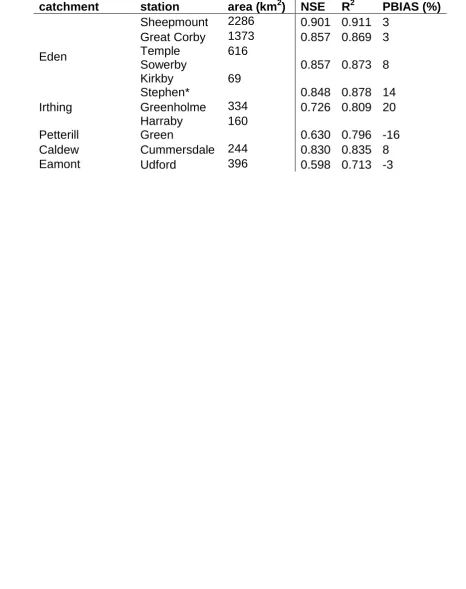
Table 4 shows the average hourly hydrological performance statistics of the 330
model for the validation period (and daily statistics at Kirkby Stephen where hourly 331
flow data were unavailable). All hourly NSE and R2 values are above 0.55 and 0.7 332
respectively, indicating satisfactory model performance at all sites (Moriasi et al, 333
2007). The simulated absolute percentage bias is below 25% at all gauging stations 334
(indicating satisfactory model performance according to Moriasi et al, 2007) and at 5 335
of the 8 stations is less than 8%. 336
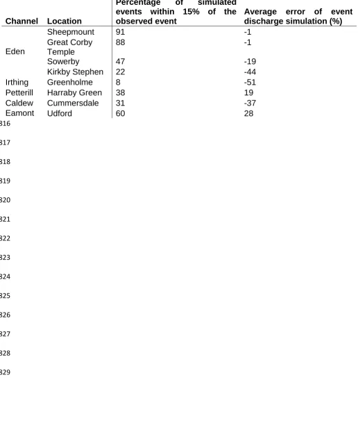
The POT analysis indicates the model’s ability to predict high-magnitude events 337
(see Figure 5 and Table 5). Although the model under-estimates event peak flow at 338
most locations, as is common with other hydrological models (Butts et al, 2004; Van 339
Liew et al, 2003), 65% of POT events were within the simulated uncertainty range at 340
the catchment outlet at Sheepmount (Table 4 and Figure 5). It should be noted that 341
the Eden at medium-high flows, which could partially explain the lower peak over 343
threshold simulation accuracy observed at this location (Table 5). 344
Bank erosion 345
The GIS overlay methodology indicates the total mass of sediment generated 346
through bank erosion processes within the catchment is between 539-2346 t yr-1 347
(Table 6). The estimates from both GIS methodologies provide an uncertainty range 348
between 211-4426 t yr-1.Total annual simulated bank erosion in Table 7 is higher 349
than the most recent observed average annual bank erosion rates (1970-2012 – 350
Table 6) but within the observed uncertainty range over the historical. Additionally, 351
Table 7 indicates the enhanced model simulates a greater inter-annual variability of 352
average annual bank erosion rates than the basic model. The enhanced model 353
simulates a greater range of spatial variation of bank erosion throughout the 354
catchment than the basic model. The basic version of the model was parameterised 355
so that the total catchment average annual mass of bank eroded sediment 356
generation was similar to the enhanced model to enable comparison of spatial bank 357
erosion simulation in Figure 6. The observed data used for comparison here is taken 358
from the upper estimate. The basic version of the model (Figure 6A) simulates a 359
fairly spatially constant magnitude of bank erosion throughout the catchment in 360
comparison to the enhanced model (Figure 6B) and the observed data (Figure 6C). 361
The model was also validated at a sub-catchment scale using Water Framework 362
Directive sub-catchment boundaries by correlating the total simulated bank eroded 363
sediment of the basic and enhanced versions of the model with the observed data. 364
Correlations between simulated and observed data indicate the enhanced model 365
provides a more accurate spatial estimation of bank erosion at the sub-catchment 366
correlation values indicate an improvement in the spatial variability of bank erosion 368
simulated by the developed model, but nevertheless the overall predictive ability of 369
the spatial variability is poor due to reasons detailed within the discussion. 370
Sediment load accuracy 371
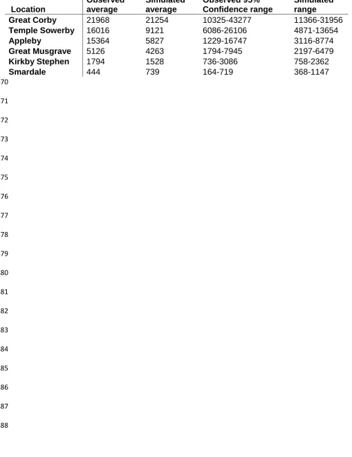
Table 8 shows observed annual sediment loads with upper and lower 95% 372
confidence intervals (calculated from the coefficient of the rating curve equations 373
from Mills, 2009), and simulated annual sediment loads with upper and lower bounds 374
based on the parameter set used for simulation. The confidence intervals of the 375
observed sediment loads incorporate both hydrological and sediment 376
parameterisation uncertainty and are of a similar magnitude to the uncertainty 377
bounds of simulated sediment loads. Furthermore, the ranges of simulated and 378
observed sediment loads overlap at all locations. 379
Sensitivity to temporal flood clustering 380
Values of bank eroded sediment generation for each of the five temporal flood 381
cluster scenarios was calculated by summing the total catchment bank erosion for 31 382
days, starting from the date of the second rainfall event (see Table 9). The model 383
indicates bank eroded sediment generated from a single flood event may be up to 384
61% greater if the event occurs within 2 weeks of a large flood event. As the 385
temporal separation of the two flood events increases the magnitude of bank erosion 386
caused by the second event decreases. Once channel bank vegetation has 387
recovered from the first event, subsequent events below the threshold discharge do 388
not result in increased magnitudes of bank erosion. 389
390
Observed bank erosion rates within this study determine the significance of 392
channel bank erosion as a sediment source within the Eden catchment, Cumbria. 393
Based on average annual simulated sediment load at Sheepmount, the data 394
collected indicate that bank erosion represents 5-11% of the annual catchment 395
sediment budget. This value is at the lower end of the range observed within other 396
UK catchments (Walling, 2005; Walling et al 2006; Bartley et al 2007) which could be 397
partly due to the predominance of grassland within the catchment. 398
The GIS dataset also indicates significant temporal variability of average annual 399
bank erosion rates between the four time-periods analysed, but does not fully 400
capture the inter-annual variability. Several previous studies have noted significant 401
inter-annual variability of bank erosion processes (Hooke, 2008; Kronvang et al, 402
2013). Simulated bank eroded sediment generation using the enhanced model 403
shows greater inter-annual variation of bank erosion rates than those of the basic 404
model (Table 7), with the highest values during the year 2005. This is expected as 405
the largest event discharge recorded during the study period (and 2nd largest to date) 406
at this station occurred during the January of this year (8/1/2005 1516.3 m3s-1). 407
Previous studies have indicated the significance of high magnitude events to bank 408
erosion (Hooke, 1979; Julian and Torres 2006; Henshaw et al, 2012; Palmer et al, 409
2014). The developed representation of bank erosion processes enables model 410
sensitivity to high magnitude events, and therefore replication of observed temporal 411
(inter-annual) variability of sediment generation. 412
The observed average annual bank erosion rates for the years 1970-2012 shown 413
in Table 6 are lower than average simulated values for 2001-2006. The observed 414
data present an average annual bank erosion value across several years and inter-415
represented. The average annual maximum discharge recorded at Sheepmount from 417
1970-2012 was considerably lower than between 2001-2006 (647m3s-1 and 764m3s-1 418
respectively). Therefore bank erosion rates between 2001-2006 would be expected 419
to be higher than the 1970-2012 average. Furthermore, observed data show total 420
bank erosion within 6 main channels of the Eden catchment, additional smaller 421
tributaries have not been included, yet simulated values include the whole catchment 422
as represented by the model. The lower estimates of observed bank erosion are 423
taken from the GIS overlay methodology with a 3.5m buffer applied to account for 424
errors within the mapping process, which for more recent maps (such as 1970 and 425
2012) should be less significant than for earlier maps. Therefore the lower estimate 426
of actual bank erosion for the 1970-2012 time-period is potentially a significant 427
underestimate of reality. 428
The enhanced model simulates sensitivity to flood clustering, by incorporating an 429
element of catchment recovery following a large event. The results indicate bank 430
eroded sediment generation for an event of the same magnitude may vary 431
depending on the event timing. Previous studies have noted the importance of 432
antecedent conditions to bank erosion processes; Hooke (1979) noted that whilst 433
event-based bank erosion at certain sites was correlated with discharge of the 434
previous peak, the influence of this variable is complex. Previous high flows can 435
weaken banks by undercutting but can also remove loose bank material leaving the 436
bank more resistant to subsequent high flows. Thorne (1982) observed that mass 437
failure of banks can result in an increase in bank stability due to supply of sediment 438
to the basal zone, unless critical shear stress for removal of this basal material is 439
exceeded. The enhanced model developed in this study provides an additional 440
of event clustering, and influence of antecedent conditions. The frequency of high 442
magnitude events within the UK is expected to increase with projected climatic 443
changes (Bell et al, 2012; Kay et al, 2014; Madsen et al, 2014). Therefore, to enable 444
climate-proof catchment management practices models will be required to represent 445
the effects of flood clustering. 446
The spatial variation of bank erosion simulated by the basic model was controlled 447
solely by flow variation (and hence variation of shear stress) throughout the 448
catchment. As shown in Figure 6A this resulted in little variation of simulated bank 449
erosion across the catchment. Significant spatial variation was observed from the 450
GIS analysis within this study (Figure 6C), and has been observed within several 451
additional UK catchments (Bull, 1997; Lawler et al, 1999). The inclusion of sinuosity 452
within the enhanced model enables simulation of some spatial variability of bank 453
erosion rates within the catchment (Figure 6B). Correlation of sub-catchment totalled 454
bank erosion rates indicate that bank erosion predicted by the enhanced model is 455
more accurate than the basic model, yet still provides a weak fit of the observed 456
bank erosion rates throughout the catchment. Several factors such as anthropogenic 457
influences, lithology, channel confinement, bank height, and slope influence bank 458
erosion rates resulting in the significant observed spatial variability within 459
catchments. Whilst sinuosity is known to be one factor influencing the spatial 460
variation of bank erosion (Janes 2013; Micheli and Kirchner 2002) many of these 461
additional factors are not included within the developed model due to current limited 462
understanding of their behaviour, complex interactions, and lack of spatial data 463
coverage. Therefore some differences between the simulated and observed bank 464
erosion rates are to be expected due to the omission of many of these factors and 465
erosion rates. Comparisons of observed and model simulated bank erosion values 467
such as those in Figure 6 are rarely performed but these types of analyses are 468
required if models are to be judged useful in management at the local scale. The 469
model can be used to assist identification of areas where bank erosion would be 470
expected to occur naturally, and comparison with observational data can indicate 471
areas where bank erosion is prevented/accelerated due to anthropogenic factors not 472
included within the model. 473
The observed bank erosion data within this study provides an estimate of annual 474
bank eroded sediment generation with greater spatial resolution and over a longer 475
timescale than is possible using field-based techniques (such as erosion pins). 476
However, it is not possible to accurately estimate event-based bank eroded sediment 477
using data derived from this methodology. Further data (such as LIDAR analysis of 478
bank migration at a finer temporal scale) and analysis is required to calibrate the 479
model and assess performance during individual events. 480
481
Conclusions 482
Channel bank erosion contributes a significant proportion of catchment sediment 483
budgets and yet is commonly excluded or overly simplified within catchment scale 484
models. In this study, the bank erosion component within the physically-based 485
SHETRAN model has been further developed to incorporate both temporal and 486
spatial variability of bank erosion by inclusion of additional controlling factors; 487
removal of bank vegetation and bank collapse after a flood event and subsequent 488
recovery, and channel sinuosity. The developments within this study improve the 489
representation of natural processes influencing bank erosion rates, and enable 490
The model has been successfully applied to the Eden catchment, north-west 492
England, and validated using hydrological, bank erosion and suspended sediment 493
data. The enhanced model has been shown to simulate improved inter-annual and 494
spatial variability of catchment scale bank eroded sediment generation when 495
compared with the basic model, yet it is noted that the developed model still provides 496
a weak fit with observed data. Differences between the spatial variation of observed 497
and simulated bank erosion rates are attributed to additional factors not included 498
within the model due to limitations in current understanding and data availability. 499
Simulated sediment loads were compared with observational data, and whilst 500
uncertainty in both observed and predicted sediment loads is large, values were 501
found to overlap throughout the catchment, indicating reasonable accuracy of model 502
simulations. Whilst the accuracy of spatial bank erosion simulations is currently 503
insufficient to support application of the model for management purposes the study 504
represents a contribution to the research need for continuing development of 505
sediment models. The developed representation of bank erosion processes that 506
have been applied to the SHETRAN model in this study could also be applied to a 507
number of existing physically based models. 508
The developed representation of sediment source estimation within the model 509
provides a more holistic representation of sediment processes throughout the 510
catchment. The resultant model provides an improved representation of the spatial 511
and temporal variability of sediment loads, yet further development of such models is 512
required to provide estimates of sediment loads with sufficient accuracy to support 513
management of diffuse pollution. 514
515
We would like to thank the two anonymous reviewers for their helpful and 517
constructive comments that assisted in improving this manuscript. This work was 518
funded by EPSRC as part of the FloodMEMORY project EP/K013513/1. Additional 519
thanks go to the Environment Agency for the provision of channel survey and bank 520
height data, Cranfield University for LandIS soil data, and the CHASM project and 521
Carolyn Mills for sediment data. The associated metadata/data presented in this 522
research can be accessed using the following DOIs: 10.17862/cranfield.rd.4300220, 523
10.17862/cranfield.rd.4300202. 524
525
References 526
Arnold, J.G., Srinivasan, R., Muttiah, R.S., Williams, J.R. 1998. Large-area 527
hydrologic modelling and assessment: Part 1. Model development. . JAWRA 528
Journal of the American Water Resources Association 34, 73-89. 529
Bathurst, J.C., Burton, A., Clarke, B.G. and Gallart, F. 2006. Application of the 530
SHETRAN basin-scale, landslide sediment yield model to the Llobregat basin, 531
Spanish Pyrenees. Hydrological Processes, 20, 3119-3138. 532
Bartley, R., Hawdon, A., Post, D.A., Roth, C.H. 2007 A sediment budget for a 533
grazed semi-arid catchment in the Burdekin basin, Australia, Geomorphology 87, 534
302-321. 535
Bartley, R. Keen, R.J., Hawdon, A.A., Hairsine, P.B., Disher, M.G., Kinset-536
Henderson, A.E. 2008. Bank erosion and channel width change in a tropical 537
environment. Earth Surface Processes and Landforms 33, 14, 2147-2200. 538
Bell, V.A., Kay, A.L., Cole, S.J., Jones, R.G., Moore, R.J., Reynard, N.S. (2012) 539
wide analysis using the UKCP09 Regional Climate Model ensemble, Journal of 541
Hydrology 442-443, 89-104. 542
Beasley, D.B. and Huggins, L.F. 1982. ANSWERS – Users manual. EPA-905/9-543
82-001, USEPA, Region 5, Chicago, IL. 544
Birkinshaw, S.J., Bathurst, J.C., Robinson, M. 2014. 45 years of non-stationary 545
hydrology over a forest plantation growth cycle, Coalburn catchment, Northern 546
England. Journal of Hydrology 519, 559-573. 547
Bull, L.J. 1997. Magnitude and variation in the contribution of bank erosion to the 548
suspended sediment load of the River Severn, UK. Earth Surface Processes and 549
Landforms 22, 1109–1123. 550
Butts, M.B., Payne, J.T., Kristensen, M., Madsen, H. 2004. An evaluation of the 551
impact of model structure on hydrological modelling uncertainty for streamflow 552
simulation. Journal of Hydrology 298, 242-266. 553
Centre for Ecology and Hydrology 2007 Land Cover Map 554
http://www.ceh.ac.uk/services/land-cover-map-2007 (accessed on 27/8/2015). 555
Centre for Ecology and Hyrdrology 2015 National River Flow Archive 556
http://nrfa.ceh.ac.uk/ (accessed on 27/8/2015) 557
Couper, P., Stott, T.I.M., Maddock, I.A.N. 2002. Insights into river bank erosion 558
processes derived from analysis of negative erosion-pin recordings: Observations 559
from three recent UK studies. Earth Surface Processes and Landforms 79, 59– 560
79. 561
Croasato, A. 2009. Physical explanations of variations in river meander migration 562
rates from model comparison, Earth Surface Processes and Landforms 34, 2078-563
Darby, S.E., Alabyan, A.M., Van de Wiel, M.J. 2002. Numerical simulation of 565
bank erosion and channel migration in meandering rivers, Water Resources 566
Research, 38. 567
Darby, S.E., Rinaldi, M., Dapporto, S. 2007. Coupled simulations of fluvial 568
erosion and mass wasting for cohesive river banks, Journal of Geophysical 569
research, 112. 570
Davison, P.S., Withers, P.J. a., Lord, E.I., Betson, M.J., Strömqvist, J., 2008. 571
PSYCHIC – A process-based model of phosphorus and sediment mobilisation 572
and delivery within agricultural catchments. Part 1: Model description and 573
parameterisation. Journal of Hydrology 350, 290–302. 574
Duan, J.G. 2005. Analytical approach to calculate rate of bank erosion, Journal of 575
Hydraulic Engineering 131, 980-990. 576
Elliott, A. H., Oehler, F., Schmidt, J. and Ekanayake, J. C. 2012. Sediment 577
modelling with fine temporal and spatial resolution for a hilly catchment. 578
Hydrological Processes. 579
Environment Agency. 1998. Revetment Techniques Used on the River Skerne 580
Restoration Project. Technical Report W83. 581
Environment Agency. 2012 WFD River Waterbodies data. 582
https://data.gov.uk/dataset/wfd-river-waterbodies Accessed 9/7/2015. 583
Ewen, J., Parkin, G., O'Connell, P.E., 2000. SHETRAN: distributed river basin 584
flow and transport modeling system. Journal of hydrologic engineering 5, 250-585
258. 586
Faulkner, D. 1999. Flood Estimation Handbook, Vol. 2: Rainfall frequency 587
Henshaw, A.J., Thorne, C.R., Clifford, N.J. 2012 Identifying causes and controls 589
of river bank erosion in a British upland catchment. Catena 100, 107-119. 590
Hickin, E., 1978. Mean flow structure in meanders of the Squamish River, British 591
Columbia. Canadian Journal of Earth Sciences 15, 1833–1849. 592
Hickin, E., Nanson, G., 1975. The Character of Channel Migration on the Beatton 593
River , Northeast British. Geological Society of America Bulletin 86, 487–494. 594
Hooke, J., 1979. An analysis of the processes of river bank erosion. Journal of 595
Hydrology 42, 39–62. 596
Hooke, J., 1980. Magnitude and distribution of rate of river bank erosion. Earth 597
surface processes 5, 143–157. 598
Hooke, J.M., 2007. Spatial variability, mechanisms and propagation of change in 599
an active meandering river. Geomorphology 84, 277–296. 600
Hooke, J.M., 2008. Temporal variations in fluvial processes on an active 601
meandering river over a 20-year period. Geomorphology 100, 3–13. 602
Jarritt, N., Lawrence, D., 2007. Fine sediment delivery and transfer in lowland 603
catchments: modelling suspended sediment concentrations in response to 604
hydrological forcing. Hydrological Processes 2744, 2729–2744. 605
Janes, V.J., Nicholas, A.P., Collins, A., Quine, T. 2017. Analysis of fundamental 606
physical factors influencing channel bank erosion: results for contrasting 607
catchments in England and Wales. Environmental Earth Sciences, in press. 608
Janes, V.J. 2013 An analysis of bank erosion and development of a catchment 609
sediment budget mode. Unpublished PhD thesis, University of Exeter. 610
Julian, J., Torres, R., 2006. Hydraulic erosion of cohesive riverbanks. 611
Geomorphology 76, 193–206. 612
Probabilistic impacts of climate change on flood frequency using response 614
surfaces 1: England and Wales, Regional Environmental Change 14, 1215-1227. 615
Knisel, W., 1980. CREAMS A field scale model for Chemicals Runoff and Erosion 616
from Agricultural Management Systems, USDA Conservation Research Report. 617
Kronvang, B., Andersen, H.E., Larsen, S.E. 2013 Importance of bank erosion for 618
sediment input, storage and export at the catchment scale, Journal of Soils and 619
Sediments 13, 230-241. 620
LandIS (2014) Soils Data © Cranfield University (NSRI) and for the Controller of 621
HMSO. 622
623
Lawler, D.M., Grove, J.R., Couperthwaite, J.S., Leeks, G.J.L., 1999. Downstream 624
change in river bank erosion rates in the Swale ± Ouse system , northern 625
England 992. 626
Lewin, G., Brindle, B., 1977. Confined Meanders, in: Gregory, K. (Ed.), River 627
Channel Changes. Wiley, pp. 221–233. 628
Lewis, E., Birkinshaw, S., Quinn, N., Freer, J., Coxon, G., Woods, R., Bates, P., 629
Fowler, H. 2016. A gridded hourly rainfall dataset for the UK applied to a national 630
physically-based modelling system, Geophysical Research abstracts 18. 631
Lukey, B.T., Sheffield, J., Bathurst, J.C., Hiley, R.A. and Mathys, N. 2000. Test of 632
the SHETRAN technology for modeling the impact of restoration on badlands 633
runoff and sediment yield at Draix, France. Journal of Hydrology, 235, 44-62. 634
Mayes, W.M., Walsh, C.L., Bathurst, J.C., Kilsby, C.G., Quinn, P.F., Wilkinson, 635
M.E., Daugherty, A.J. and O'Connell, P.E. (2006), Monitoring a flood event in a 636
densely instrumented catchment, the Upper Eden, Cumbria, UK. Water and 637
Environment Journal, 20: 217–226. doi:10.1111/j.1747-6593.2005.00006.x 638
A.J., Zaharia, S. 2003 The long term fate and environmental significance of 640
contaminant metals released by the January and March 2000 mining tailings dam 641
failures in Maramureş County, upper Tisa Basin, Romania. Applied Geochemistry 642
18, 241-257. 643
Madsen, H., Lawrence, D., Lang, M., Martinkova, M., Kjeldsen, T.R. (2014) 644
Review of trend analysis and climate change projections of extreme precipitation 645
and floods in Europe, Journal of Hydrology 519, 3634-3650. 646
Mcintyre, N., Ballard, C., Bulygina, N., Frogbrook, Z., Cluckie, I., Dangerfield., S., 647
Ewen, J., Geris, J., Henshaw, A., Jackson, B., Marshall, M., Pagella, T., Park, 648
J.S., Reynolds, B., O;Connel, E., O’Donnell, G., Sinclar, F., Solloway, I., Thorne, 649
C., Wheater, H. (2012) The potential for reducing flood risk through changes to 650
rural land management: outcomes from the Flood Risk Management Research 651
Consortium, BHS Eleventh National Symposium, Dundee. 652
Michalková, M., Piégay, H., Kondolf, G.M., Greco, S.E., 2011. Lateral erosion of 653
the Sacramento River, California (1942-1999), and responses of channel and 654
floodplain lake to human influences. Earth Surface Processes and Landforms 36, 655
257–272. 656
Micheli, E., Kirchner, J., 2002. Effects of wet meadow riparian vegetation on 657
streambank erosion. 1. Remote sensing measurements of streambank migration 658
and erodibility. Earth Surface Processes and Landforms 27, 627– 639. 659
Mills, C. 2009 Spatial variability and scale dependency of sediment yield in a rural 660
river system – the river Eden, Cumbria, UK. Newcastle University, UK. 661
Unpublished PhD thesis. 662
Moriasi, D.N., Arnold, J.G., VanLie, M.W., Bingner, R.L., Harmel, R.D., Veith, T.L. 663
watershed simulations. Transactions of the ASABE 50, 885-900. 665
Nagata, N., Hosoda, T., Muramoto, Y. 2000. Numerical analysis of river channel 666
processes with bank erosion, Journal of Hydraulic Engineering 126, 243-252. 667
Ordnance Survey (2009) OS land-form PANORAMA DTM, 1:50000. Digimap: 668
EDINA supplied service, available at: htt[://digimap.edina.ac.uk/ 669
Owens, P.N., Batalla, R.J., Collins, A.J. Gomez, B., Hicks, D.M., Horowitz, A.J., 670
Kondolf, G.M., Marden, M., Page, M.J., Peacock, D.H., Pettocrew, E.L., 671
Salomons, W., Trustrum, N.A. 2005. Fine-grained sediment in river systems: 672
environmental significance and management issues, River Research and 673
Applications 21, 693-717. 674
Owens, O.N., Walling, D.E. 2002. The phosphorus content of fluvial sediment in 675
rural and industrialized river basins, Water Research, 36, 685-701. 676
Palmer, J.A., Schillling, K.E., Isenhart, T.M., Schultz, R.C., Tomer, M.D. 2014 677
Streambank erosion rates and loads within a single watershed: Bridging the gap 678
between temporal and spatial scales, Geomorphology 209, 66-78. 679
Perry, M., Hollis, D., Elms, M. 2009. The generation of daily gridded datasets and 680
rainfall for the UK, Climate Memorandum 24. Met Office. National Climate 681
Information Centre. Exeter, UK. 682
Prosser, I., Young, I., Rustomji, P., Hughes, A., Moran, C., 2001. A Model of 683
River Sediment Budgets as an Element of River Health Assessment, in: 684
International Congress on Modelling and Simulation. pp. 1–6. 685
Rhoades, E.L., O’Neal, M.A., Pizzuto, J.E. 2009 Quantifying bank erosion on the 686
South River from 1937 to 2005, and its importance in assessing Hg 687
Rowan, J.S., Barnes, S.J.A., Hetherington, S.L., Lambers, B., Parsons, F. (1995) 689
Geomorphology and pollution: the environmental impacts of lead mining, 690
Leadhills, Scotland. Journal of Geochemical Exploration 52, 57-65. 691
Sharpley, A.N. and Williams, J.R. (Editors), 1990. Epic-Erosion/Productivity 692
Impact Calculator: 1. Model Documentation. U.S. Dept. ofAgric. Tech. Bul. No., 693
176-235 pp. 694
Simon, A., Curini, A., Darby, S.E., Langendoen, E.J. 2000. Bank and near-bank 695
processes in an incised channel. Geomorphology 35, 193-217. 696
Simon, A., Collison, A., 2002. Quantifying the mechanical and hydrologic effects 697
of riparian vegetation on streambank stability. Earth Surface Processes and 698
Landforms 27, 527–546. 699
Soulsby, C., Youngson, A., Moir, H., Malcolm, I.A., 2001. Fine sediment influence 700
on salmonid spawning habitat in a lowland agricultural stream: a preliminary 701
assessment. Science of the Total Environment 265, 295–307. 702
Surian, N., Mao, L., 2009. Morphological effects of different channel‐forming 703
discharges in a gravel‐bed river. Earth Surface Processes and Landforms1107, 704
1093–1107. 705
Thorne, C.R. 1982 Processes and mechanisms of river bank erosion, in
Gravel-706
Bed Rivers, Hey, R.D., Bathurst, J.C., Thorne, C.R. (eds) Wiley, Chichester. 707
Van Liew, M., Arnold, J.G., Garbrecht, J.G., 2003. Hydrologic sumulation on 708
agricultural watersheds: Choosin between two models. Transactions of the ASAE 709
46, 1539–1551. 710
Walling, D.E., 2005. Tracing suspended sediment sources in catchments and 711
Walling D.E., Collins, A.L., Jones, P.A., Leeks, G.J.L., Old, G. 2006 Establishing 713
fine-grained sediment budgets for the Pang and Lambourn LOCAR catchments, 714
UK, Journal of Hydrology 330, 126-141. 715
Walling, D.E., Collins, A.L., Stroud, R.W., 2008. Tracing suspended sediment and 716
particulate phosphorus sources in catchments. Journal of Hydrology 350, 274– 717
289. 718
Wilkinson, S.N., Prosser, I.P., Rustomji, P., Read, A.M. 2009. Modelling and 719
testing spatially distributed sediment budgets to relate erosion processes to 720
sediment yields, Environmental Modelling and Software 24, 489-501. 721
Winterbottom, S.J., Gilvear, D.J., 2000. A GIS-based approach to mapping 722
probabilities of river bank erosion: regulated river Tummel, Scotland. Regulated 723
Rivers: Research & Management 16, 127–140. 724
Wösten, J.H.M., Lilly, A., Nemes, A., Le Bas, C. 1999 Development and use of a 725
database of hydraulic properties of European soils. Geoderma 90, 169-185. 726
727
728
729
730
731
732
733
734
735
736
738
739
740
Table 1: Model user input parameters required for the developed bank erosion 741
model. Parameter QThresh is scaled to the outlet value.
742
Parameter Units Description
BKBmin kg m-1 s-1 Minimum bank erodibility
BKBmax kg m-1 s-1 Maximum bank erodibility
QThresh m3 s-1
Threshold discharge at which BKB for the link increases from BKBmin to BKBmax
k N/A
Vegetation recovery speed (high values = rapid growing vegetation types)
743
744
745
746
747
748
749
750
751
752
753
754
755
756
757
758
760
761
Table 2: Calibrated parameter values of the bank erosion model. 762
Parameter
Calibrated value
Return period of QThresh 12
k 0.03
Factoral difference between BKBmin and
BKBmax 20
763
764
Straight channels
Meandering channels
Highly sinuous channels
Sinuosity <1.2 1.2-1.5 >1.5
BKBmin 3.5E-11 9.6E-11 7.0E-11
BKBmax 7.0E-10 1.9E-09 1.4E-09
765
766
767
768
769
770
771
772
773
774
775
776
777
778
780
781
Table 3: Validated parameter values for the Eden catchment model. 782
Parameter/function Low
value
High value
Hydrological
Strickler overland flow resistance coefficient 1 3 Saturated hydraulic conductivity in channel soil (mm day-1) 0.1 60 Channel bank Strickler coefficients (x and y directions) 20 30
Sediment
Overland flow erodibility (kg m-2 s-1) 0.02 0.05
Raindrop impact erodibility (J-1) 2E-12 1E-11
783
784
785
786
787
788
789
790
791
792
793
794
795
796
Table 4: Average performance statistics from the simulation of hourly flows 798
across the Eden catchment (with the exception of Kirkby Stephen based on 799
daily flows) during the validation period. 800
Catchment/sub-catchment
Gauging station
Upstream
area (km2) NSE R2 PBIAS (%)
Eden
Sheepmount 2286 0.901 0.911 3 Great Corby 1373 0.857 0.869 3 Temple
Sowerby
616
0.857 0.873 8 Kirkby
Stephen*
69
0.848 0.878 14 Irthing Greenholme 334 0.726 0.809 20
Petterill
Harraby Green
160
0.630 0.796 -16
Caldew Cummersdale 244 0.830 0.835 8
Eamont Udford 396 0.598 0.713 -3
801
802
803
804
805
806
807
808
809
810
811
[image:34.595.57.524.169.759.2]Table 5: Percentage of peak over threshold events within the simulated range 813
during the validation period, and average percentage error of simulated peak 814
discharge. 815
Channel Location
Percentage of simulated events within 15% of the observed event
Average error of event discharge simulation (%)
Eden
Sheepmount 91 -1
Great Corby 88 -1
Temple
Sowerby 47 -19
Kirkby Stephen 22 -44
Irthing Greenholme 8 -51
Petterill Harraby Green 38 19
Caldew Cummersdale 31 -37
Eamont Udford 60 28
816
817
818
819
820
821
822
823
824
825
826
827
828
Table 6: Observed bank erosion rates (t yr-1) from each overlay time period. 830
Values shown are averages from all methodological estimates, 831
832
Channel 1880-1901 1901-1956 1956-1970 1970-2012
Eden 1329 682 1612 198
Petteril 136 58 209 29
Caldew 412 187 439 117
Irthing 356 216 487 166
Lyvenet 55 26 59 12
Eamont 58 17 44 16
Total 2346 1186 2849 539
833
834
835
836
837
838
839
840
841
842
843
844
845
846
Table 7: Annual bank erosion for the whole catchment as simulated by both 848
the basic and enhanced models during the validation period. Values are in t yr -849
1 . 850
2001 2002 2003 2004 2005 2006
Enhanced
Minimum 721 1655 617 1686 2842 622
Maximum 4063 2833 2219 2682 3898 2784 Average 2331 2120 1401 2093 3350 1400
Basic
Minimum 1951 3170 1542 2907 2356 2943 Maximum 2126 3355 1728 3129 2539 3183 Average 2001 3234 1588 2972 2404 3013 851
852
853
854
855
856
857
858
859
860
861
862
863
864
865
866
867
[image:37.595.46.531.150.770.2]Table 8: Observed and simulated average annual sediment loads (t yr-1). 869
Location
Observed average
Simulated average
Observed 95% Confidence range
Simulated range
Great Corby 21968 21254 10325-43277 11366-31956
Temple Sowerby 16016 9121 6086-26106 4871-13654
Appleby 15364 5827 1229-16747 3116-8774
Great Musgrave 5126 4263 1794-7945 2197-6479
Kirkby Stephen 1794 1528 736-3086 758-2362
Smardale 444 739 164-719 368-1147
870
871
872
873
874
875
876
877
878
879
880
881
882
883
884
885
886
887
Table 9: Model sensitivity to temporal sequencing of flood events. Bank 889
erosion values shown are summed from the whole catchment over a period of 890
31 days, starting from the beginning of the second rainfall event. 891
Time between flood events (weeks)
Monthly bank erosion during second event (t)
1 851
2 681
4 547
6 536
8 530
12 528