A Measure of Dynamic Market Performance
René Y. Darmon1*, Louis Duclos-Gosselin2, Benny Rigaux-Bricmont3
1Marketing Department, ESSEC Business School, Cergy-Pontoise, France; 2Analyse des Modes de Défaillance, de Leurs Effets et de Leurs
Criticités, Quebec City, Canada; 3Marketing Department, Faculty of Administration Sciences, Laval University, Quebec City, Canada.
Email: *[email protected], [email protected], [email protected]
Received November 9th, 2012; revised December 17th, 2012; accepted January 18th, 2013
Copyright © 2013 René Y. Darmon et al. This is an open access article distributed under the Creative Commons Attribution License, which permits unrestricted use, distribution, and reproduction in any medium, provided the original work is properly cited.
ABSTRACT
This paper proposes an easy-to-implement dynamic measure of market performance over time for various selling units (e.g., sales territories, sales regional offices, or the whole sales organization). It may be used as a diagnosis tool by comparing the market performances of various units, taking into account the conditions prevailing in the different mar- kets (such as competition relative effectiveness, sales penetration, or local market fluctuations). Combining sales vol- ume, market share, and profit variations data into an Index of Sales Unit Market Performance (ISUMP), provides managerial guidance for selling units’ evaluation or resource allocations among units. This index may account for a firm’s selected market strategy (market penetration, market skimming, etc.). Implementation in a large North American insurance company is reported.
Keywords: Selling Units; Market Performance; Sales Performance; Market Shares; Selling Unit Control
1. Introduction
Many managerial marketing decisions (e.g., budget and resource allocations) and sales force decisions aim at maintaining or improving the performance of various
selling units over time [1-3]. A selling unit is an entity responsible for achieving some output market perfor- mance. It may be, for instance, a sales territory (either assigned to a sales team or to an individual salesperson), a regional or district sales office, or the whole sales or- ganization. Every selling unit is characterized by its mar- ket output performance (such as sales, profits, or market share) that results from the accomplishment of the selling tasks, in a specific environment, over some long- and/or short-term period of time.
In order to effectively manage and control selling units, managers must rely on valid and accurate measures of market performance [4]. Inaccurate assessments may lead to poor managerial decisions, feelings of inequity, morale problems, lack of organizational commitment, and dysfunctional turnover [5-8]. For that purpose, managers generally collect and analyze large amounts of data, often frequently supplied by CRM applications. However, it is often difficult to devise adequate measures of market performance [9]: this concept covers, among
others, short- and long-term variations in sales, profits, customer satisfaction, loyalty building, and customer re- lationship development; it is multidimensional [9,10] and consequently, no single measure can account for its va- rious dimensions. This is exemplified by the large num- ber of definitions and measures used for that purpose [2,3], that range from managerial subjective judgments and self-assessments [6] to simplistic measures, like sales volumes [10]. A meaningful measure of market perfor- mance should capture the extent to which a selling unit is able to take advantage of market opportunities (or lack thereof) in order to achieve a firm’s desired market po- sition and implement its selling strategy. Managers often lack such simple measures.
The aim of this paper is to devise a measure of a sell- ing unit’s market performance over time that could sup- plement the management’s control tool kit. When con- sidered jointly with extra-role performance measures [11], this market performance measure allows managers to make better diagnoses, and consequently, to provide better managerial guidance for selling units’ evaluation, organization, compensation, and/or resource allocations [12].
nally, the advantages and limits of this procedure are discussed.
2. Selling Units’ Market Performance
Measures
Assessing market performance is fraught with difficulty, and sales force researchers and sales managers have ty- pically used different approaches to that purpose [13- 21].
2.1. Sales Force Researchers’ Approaches
Over the last decades, a major stream of sales force re- search has attempted to gain better understanding of salespeople’s performance and to find appropriate ways to enhance selling effectiveness [22]. The seminal work by [23] that proposed a model of the major determinants and consequences of sales force performance has been followed by many studies sharing similar concerns [24- 29]. These studies have investigated the antecedent and/ or consequences of salespeople’s sales performance and/ or effectiveness [30-32].
In most cases, researchers have measured selling units’ performance either using objective sales data [11] or eva- luative scales [6]. Measurement instruments have been completed by managers, by salespersons themselves (self- reports) [12,33-35], or both [36-38]. It seems that, in prac- tice, research suggests that subjective and objective meas- ures lead to different results [39-44]. Unfortunately, be- cause they are highly subjective and may well yield bias- ed judgments [45,46], their validity is often questionable [44,47], and they can have only limited practical value. Consequently, such self-report evaluative scales are sel- dom used alone in the practice of sales management.
2.2. Sales Managers’ Approaches
In order to assess selling unit market performance, mana- gers have typically used quantitative and/or qualitative measures [48]. Here again, the former measures (such as sales volume) tend to be objective and easy to assess. Unfortunately, they seldom capture the qualitative as- pects of the selling job, especially the extra-role perfor- mance aspects [11]. In addition, they are inadequate for assessing the unit’s performance over time, taking into account the effects of environmental variables on market size. A selling unit’s sales performance results from ma- ny other factors than the marketing resources deployed in this unit [49], for instance, each unit’s environmental conditions (competitive strength, economic conditions, etc.).
Alternatively, in order to explain management controls of the sales force, some authors have made a distinction between behavior- and outcome-based sales force con-
trols [50-52]. Although controlling salespeople’s be- haviors is an important and necessary aspect of sales management [53,54], it would be worthless if the proper behaviors did not eventually translate into sales, profits, market shares, strengthened customer relationships, or clients’ satisfaction. In practical situations, managers do evaluate selling unit market performance from at least some objective quantitative measures of sales perfor- mance [55], and outcome performance is always part of a sales force control process [56-58]. Although outcome performance measures are always used by management, few, if any, can provide a fair assessment of a sales unit’s market performance.
Territory sales volume, market shares, or profits, which are typically observed by managers, are inadequate market performance measures when considered indi- vidually. As stated above, although selling units are instrumental in building sales volume over time, sales are also influenced by a host of factors which are beyond the unit’s control. In most cases, managers cannot easily disentangle what parts of such outcomes must be attri- buted to a selling unit’s marketing program (attractive- ness of the offers, advertising, company’s reputation, etc.), or to environmental factors (competitive strength, economic trends, etc.). As a result, sales volume alone may give a distorted picture of this unit’s market per- formance [35,59]. Although territory market shares bring the additional dimensions of industry sales, competition’s performance, and the firm’s market penetration, they suf- fer from the same problems as sales volume. In addition, all outcome measures of performance tend to over-em- phasize short-over long-term performances. Finally, sell- ing unit profit measures are useful to watch, in as much as the units are given responsibility to negotiate prices and/or are left to allocate their efforts and resources among several product lines with different profit margins [60]. Being linked to sales, profit measures have the same drawbacks as sales, as market performance meas- ures.
Sales variations over some benchmark period (after removing seasonal effects) are frequently used and pro- vide better measures because they indicate a unit’s suc- cess (or failure) in sustaining a given level of sales over time. Taken alone, however, sales variations can be mis- leading because they may also be caused by many factors beyond a selling unit’s control (for instance, a shift in territory environmental conditions, windfall sales in any of the two periods, or simply random factors affecting sales in one or both periods of time).
suggests that salespersons’ confusion can result from control systems that combine both customer satisfaction and short-term performance measures such as sales [61]. Not surprisingly, a survey has shown that only a re- latively small proportion of firms (about 25 percent) use customer satisfaction as a basis for selling unit per- formance evaluation and rewards [62].
Market share variations in a selling unit’s territory provide a clear indication of a firm’s standing in its market. It measures a company’s market penetration, and, to some extent, the selling unit is responsible for it. Market share brings the additional dimension of industry sales, and consequently, of competitive performance. Com- petitive sales performance constitutes a natural bench- mark for evaluating selling units’ market performances. In other words, it is essential to account for the evolution of the competition’s sales levels for evaluating selling unit market performance.
When territory sales, industry sales, market shares,
and profit variations are considered jointly, they provide a more complete assessment of a selling unit market performance. Various market conditions require different efforts and abilities [36]. Increasing or even maintaining sales volume and/or profits in a declining market are indicative of higher market performance than the same achievement in a fast expanding market. A few methods, such as data envelopment analysis (DEA) [14,63] have been proposed and sometimes used in practice for ad- dressing the problem of evaluating selling units’ market performance with multiple criteria [64]. This technique relies on linear aggregations of various inputs and out- puts and compares every selling unit to the “best” per- forming one. It has, however, a number of limitations, the most serious ones being its complexity and difficulty to make it understood by practitioners, its reliance on many subjectively selected criteria, and its sensitivity to measurement errors [14].
Another important dimension of selling unit market performance is the time frame over which it is measured. While building long-term relationships with customers has become a prevalent strategy, short-term sales have often become inadequate measures of market perfor- mance. The current emphasis on sales activity based at the expense of outcome-based controls is a logical con- sequence of this evolution. Consequently, there is a need for devising selling unit’s market performance measures that 1) are meaningful to managers, 2) are based on easily observable and quantifiable data, 3) are valid and reflect the ability of selling units to progress, taking into account its market evolution, and 4) can accommodate short- as well as long-run market performance assess- ments.
Like DEA, the selling unit market performance meas- ure used in this study is also a multi-criterion procedure.
It presents, however, several advantages over DEA: 1) it measures “true” market performance, discarding environmental factors that influence the sales results of every selling unit; 2) unlike DEA which is an ex- treme point method, it is not sensitive to some unusu- ally high or low unit performances, and consequently to outlying observations; 3) it requires much less com- putations (against one linear program per selling unit in DEA); and 4) it is more easily understood and ap- plicable by managers.
3. Method
3.1. PrincipleManagers assess a selling unit’s market performance at time T1 by comparing the performance this unit has
achieved over some period of time t (typically a few weeks or months, ending at time T1) to some selected
benchmark. Depending on the situation and manage- ment’s goals, the selected benchmark can be 1) the outcomes achieved during a comparable reference period of length t (such as the preceding period T0 or some other
selected period, or an average of several selected bench- mark periods), or 2) some target outcome levels to be achieved during the considered period of time (for in- stance, some sales objectives or quotas). The analysis can be carried with one or several types of appropriate bench- mark.
The choice of a benchmark is crucial and requires careful managerial consideration. Selecting a preceding similar period is appropriate whenever, during this period of time, external factors have not differentially and sig- nificantly affected the various selling units.
At some time T1, four main factors reflect different
aspects of a selling unit’s current market performance variation over the benchmark: 1) the total industry sales (IS) variation in this unit: 1
1 0
0; although a selling unit cannot be held responsible for industry sales variations, one should recognize that it is more difficult to improve a firm’s market position in a de- clining than in an expanding market; 2) the unit’s sales volume (S) variation– is IS IS IS
1 1 0 0
s S –S S over the bench- mark situation; and 3) the corresponding selling unit’s market share (MS) variation
1 1 0 0
1 1 0 0 0 0
– –
ms MS MS MS
S IS S IS S IS
,
because performance should account for a selling unit’s ability to improve or maintain the firm’s market position in its territory; and 4) the corresponding gross profit variations π1
1– 0
0. Being measures of vari- ation (in decimal form), is1, s1, ms1, and π1 can either bebetween −1 and +∞1.
In order to provide a simpler explanation of the un- derlying concepts and rationale of the proposed method, a simpler case that does not consider profit variations is discussed first. Then, in a following section, the method is generalized to the case including profit variations.
3.2. Selling Units’ Market Performance (Excluding Gross Profits)
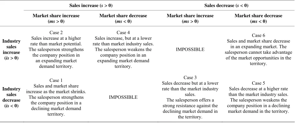
Table 1 provides an eight-cell cross-tabulation of selling
units’ market performance situations according to the variation directions of the territory’s industry sales (is1 >
0 or < 0), sales volumes (s1 > 0 or < 0), and market share
(ms1 > 0 or < 0). (From here on, for simplification pur-
pose, the subscript 1 will be omitted, unless necessary.) These three dimensions are somewhat interrelated. In- creased sales in a decreasing industry sales territory im- ply an increased market share (Case 1). Decreased sales in an increasing industry sales market imply a decreased market share (Case 6). No inference about market share variations can be made, however, on the basis of sales and industry sales variations alone when both sales and market industry sales increase (decrease). In such cases, market share increases or decreases, depending on the relative sizes of the sales and industry sales increase (de- crease) rates. Therefore, one should explicitly take mar- ket share variations into consideration. The six possible cases defined in Table 1 provide clear indications about
how a selling unit market position has evolved in its ter- ritory over time, taking into account factors over which this unit has no control (such as market size variation, competitive strength, or other factors).
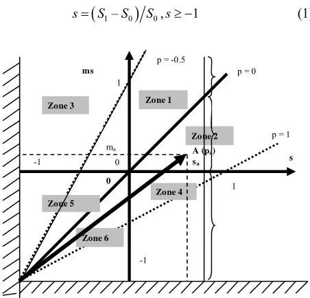
The six situations described above are represented graphically in Figure 1 (Zone 1 to 6). This diagram re-
lates a selling unit’s territory sales (s) and market share (ms) variations over the benchmark. For instance, a sell- ing unit A may have experienced a sales increase (sa) and a market share increase (msa) and consequently be posi- tioned at point A in Figure 1. The slope of the vector NA
reflects the corresponding industry sales variation (isa) during that period of time. Note that every selling unit’s vector must start at point N (−1, −1) (a 100% sales de-
crease always implies a 100% market share decrease). Because industry sales variations are generally beyond their control, selling units cannot choose the slope of the vector along which they can move. However, how far they move on their respective vectors in the direction of the arrow does reflect the quantity and quality of the work accomplished by the firm in this territory. The
length of the vector NA reflects Selling Unit A’s market performance. In other words, the unit’s market perfor- mance (the length of Vector NA) has been disentangled from uncontrollable market size variations (the slope of Vector NA).
Although theoretically, s, is, and ms can possibly vary between −1 and infinity, in most usual cases, their values are likely to be relatively close to zero (NO = status quo,
i.e., no change over the benchmark: s = is = ms = 0). The six zones shown in Figure 1 correspond to the six cases
in Table 1. Because the length of the vector is character-
istic of a given selling unit market performance, iso- market performance curves are quarter of circles centered on N. A larger radius of the circle reflects a higher mar- ket performance level.
In order to compare the market performance of various selling units, one can compare the percentages by which each one has moved on its vector compared with the
status quo N0. A formal measure called ISUMP (Index of Selling Unit Market Performance) can be used to that effect.
3.3. Analytical Formulation
Let successively be sales variations (s), industry sales variations (is) and market share variations (ms) in Selling Unit i’s territory (all in decimal form) (subscript i omit- ted unless necessary):
1– 0
0,s S S S s 1 (1)
ms
p = -0.5
Zone 1
p = 0
Zone 2 p = 1
-1
ma
0 Zone 3
Zone 4 Zone 5
Zone 6
1
s
-1
1
A (pa)
sa 0
1All the selling units are assumed to make at least some profit in T0and T1. In some relatively rare instances, however, it may be possible to observe π1 < −1 whenever a loss rather than a profit occurs in either T0 or T1. In such cases, a profit (or loss) percentage variation is meani-ngless. Whenever this situation arises, the problem can be handled in different ways: 1) excluding such selling units from this analysis and dealing with them separately; 2) If the loss is small and affects a rela-tively small number of selling units, the profit variation can be ap-proximated by the −1 value (this would slightly overestimate these selling units’ market performance); 3) the reference period could be changed (or replaced by objectives) in order to suppress the problem; and 4) the same profit amount could be added to the profit results in T0 and T1 for all the selling units, in such a way as to suppress the loss for
[image:4.595.310.536.501.718.2]Table 1. Six possible strategic performance situations according to territory sales, market industry sales, and market share variations.
Sales increase (s > 0) Sales decrease (s < 0)
Market share increase (ms > 0)
Market share decrease (ms < 0)
Market share increase (ms > 0)
Market share decrease (ms < 0)
Industry sales increase
(is > 0)
Case 2
Sales increase at a higher rate than market potential. The salesperson strengthens
the company position in an expanding market
demand territory.
Case 4
Sales increase, but at a lower rate than market industry sales.
The salesperson weakens the company position in an expanding market demand
territory.
IMPOSSIBLE
Case 6
Sales and market share decrease in an expanding market. The salesperson cannot take advantage
of the market opportunities in the territory.
Industry sales decrease
(is < 0)
Case 1 Sales and market share increase as the market shrinks.
The salesperson strengthens the company position in a declining market demand
territory.
IMPOSSIBLE
Case 3
Sales decrease but at a lower rate than the market industry
sales. The salesperson offers a strong resistance against the declining market demand in
the territory.
Case 5
Sales decrease at a higher rate than the market industry sales. The salesperson weakens the company position in a declining
market demand in the territory.
1 0
0,is IS IS IS is 1 (2)
1– 0
0,ms MS MS MS ms 1, (3) with MS0S IS0 0, and MS1S IS1 1,
where:
1 sales level achieved by Selling unit i in period 1,
in dollars; S
0 sales level for this unit in the benchmark situation,
in dollars; S
1
IS industry sales in period 1, in dollars;
0
IS industry sales in the benchmark situation, in dollars;
1
MS market share achieved in this unit’s territory in period 1, in decimal form;
0
MS market share for this selling unit’s territory in the benchmark situation, in decimal form.
Replacing S1 and IS1 by their values in (1) and (2) in
Equation (3) leads to:
1 1 1
ms is sis is (4)
Given specific values of is
1 is
, one can de- termine the linear relationship linking market share ms to sales volume s variations, as shown in Equation (4). Thus, for is 1,ms ; for is 1 2,ms2s1; for is = 0, ms = s, and for is1,ms s 2 1 2 . In the same way, because the three concepts are interrelated, each one can be expressed as a function of the other two:
1
and
1
s ms is is is s ms ms (5)
As shown in Figure 1, every selling unit can move
along a vector characteristic of its territory situation, and market performance is reflected by the position an entity has reached on its vector. By simple application of the
Pythagorean Theorem, the status quo (benchmark situa- tion) iso-performance curve has a radius equal to the square root of 2, i.e. (2)½.
In order to compare the market performance achieved by various selling units, one must assess by which per- centage each unit has moved on its vector from the status quo. For a given unit i which has achieved sales varia- tions of si0 and market share variation of msi0 in period 1,
the market performance increase (or decrease) in com- parison with the benchmark situation 0 (or Index of Sell- ing Unit Market Performance, ISUMP) is given by:
2 2
1 20 0
ISUMP 100 1si 1 msi 2 (6)
By replacing si0 and msi0 by their values in (1 - 3) and
rearranging the terms leads to another expression of the ISUMP:
1 22 2
1 1 0 1 0
ISUMP
100 IS S S IS IS 2
(7)
ISUMP = 100 means no market performance improve- ment, ISUMP > 100, some improvement, and ISUMP < 100 some market performance decrease. In order to as- sess how a selling unit’s market performance compares with the overall higher order entity (e.g., a given sales territory within its corresponding branch office) market performance, this index can be supplemented by an ad- justed ISUMP defined as2:
100 entity s ISUMP
Adjusted ISUMP
higher order entity s ISUMP
’
’ (8)
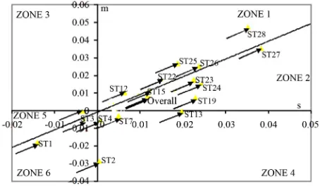
The analysis can be supplemented by locating the po- sition of every selling unit on the six-zone map (tips of market performance vectors in Figure 2). For instance,
in the reported application (see the following section), the market performance vectors of twenty-eight sales territories (ST1 to ST28) constituted of a 713 salesperson sales force have been cast into one single common graph and can be compared directly. For greater visibility, however, only representative cases from each zone are shown in Figure 2.
3.4. Selling Units’ Market Performance (Including Gross Profits)
The same principles apply when profit margin variations are added to the analysis. In this case, there are twelve situations (and twelve corresponding zones); each case identified in Table 1 being characterized either by a
profit margin (pm) increase or decrease over the bench- mark. Consequently, all previous zones are split accord- ing whether they are characterized by a profit margin increase (indexed a) or a profit margin decrease (indexed
b). As shown in Figure 3, the market performance vec-
[image:6.595.59.286.382.514.2]tors are cast into a three dimensional space characterized
Figure 2. Positions (tips of market performance vectors) of seventeen selected sales manager on the six-zone grid and overall office (darker arrow).
Figure 3. Selling unit’s market performance vector in a three dimensional space.
by the s, ms, and pm variations.
There are two ways through which a selling unit can increase profits: increasing sales and/or the profit mar- gins on the goods or service sold (either through negotia- tion of higher prices and/or selling more profitable prod- ucts). The profit situation is therefore characterized by:
1 1 0 0 0 0 0 1 1
π – , with PM S and PM S1
(9) where PM0 and PM1 are the profit margin rates respec-
tively in the benchmark situation and achieved in Period 1. Defining the profit margin variation as
1 0
pm PM PM PM0
leads to:
π pm pms s or pm π s s1 (10) A simple extension of the previous analysis leads to an estimate of the Index of Selling Unit Market Perform- ance (ISUMP):
2 2 2
1 20 0 0
ISUMP 100 1msi + 1si 1 pmi 3
(11) or using Equation (10):
1 22 2 2 2
0 0 0
ISUMP
100 1 msi 1 si + 1 π 1 si 3
(12)
3.5. Market Strategy Implementation Performance
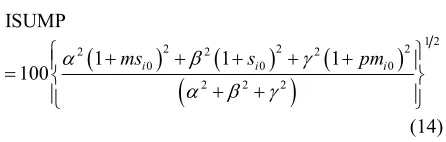
In many cases, a firm may equally value sales, market share, and profit achievement. Alternatively, when in- troducing a new product line, a firm may select a strategy of fast market penetration. In this case, sales and market shares may be assigned a higher weight than immediate profits. In other instances, the firm may select a market skimming strategy. In this case, profits may be given more importance relative to market share. Other strate- gies may be pursued. In such cases, selling units that are given the responsibility to implement market strategies, and it seems natural to assess the units’ market perform- ance at implementing them. This issue can be easily han- dled by management assigning different weights reflect- ing the relative importance of the three outcomes. Let:
weight assigned to market share increases weight assigned to sales volume increases weight assigned to profit margin increases with
1
(13)
[image:6.595.63.278.564.708.2]
1 2
2 2
2 2 2
0 0 0
2 2 2
ISUMP
1 1 1
100 msi si pmi
2
(14) In addition, when management wishes to assess selling units’ performance at implementing different market stra- tegies for different product lines, the analysis may be carried out for the various product lines separately. Then, management may assign different weights to the product lines reflecting their relative strategic importance. A weighted market performance index is computed for every unit, and compared to the corresponding higher le- vel selling entity’s ISUMP.
4. Application
This procedure has been implemented in a large North- American insurance company which sells directly to cus- tomers with no intermediary involved. Like many North American insurance companies, this firm lacked ade- quate means to properly assess the market performance of the various selling units (sales agents and sales ma- nagers) at developing their territories over time. Thus, the general sales manager was highly concerned about the current market performance evaluation procedure where sales managers were essentially relying on one single criterion, i.e., the sales volume achieved in each territory. As a result, several salespersons grew dis- satisfied with this criterion: they argued that even though their sales grew slowly (or even decreased) their territory market share was increasing. Market share data were collected from internal services and communicated to the sales personnel each month.
In this case, the application involved all the branch offices covering the North American market. The com- pany used 713 insurance agents under the supervision of sales managers in 28 sales territories. Because of space constraints, only the results of the 28 sales offices are reported here. In other words, the branch office has been selected as the selling unit. For that purpose, the required data are the summated results across territories belonging to a selling unit. Those were calculated by cumulating the results of the insurance agents they supervise.
4.1. Cross-Sectional Market Performance Analysis
Selecting an adequate time period length to assess per- formance variations is an important decision. Too short a period of time (e.g., monthly data) could lead to wide market performance variations and may hide the true longer term performance of some selling units. Alterna-
tively, too long a period of time (e.g., more than one year) may not be flexible enough, especially if management bases some financial rewards on short-term performance. This is why it may be worthwhile to carry the analysis with various time period lengths, whenever possible. In this application, quarterly performance results were not judged by management to be stable enough. Conse- quently, a one-year time period length (t = one year) was deemed most appropriate.
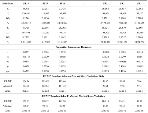
In addition, management selected market perform- ances achieved during the previous year as benchmarks for comparing current market performances. During that year, no new product had been launched, marketing in- vestments had been normal and the market had remained pretty stable. For illustration purpose, for a sample of sales territories at both ends of the performance spectrum (ST1-ST3 and ST26-ST28), the first eight rows of Table 2 give the sales levels, industry sales (estimated by the
internal services of the company), the territory market shares, and the gross profit margins during both Year 1 (Y1) and Year 2 (Y2), with Y0 as thebenchmark situation.
The percentage variations (in decimal form) in sales (s), industry sales (is), market shares (ms), gross profits (π) and gross profit margins (pm) in Year 2 over Year 1 have been used for computing the Index of Selling Unit Market Performance (ISUMP), using Equation (11) or (12). In this application, gross profit margins were esti- mated as:
Gross profit marginsrevenues sales cost general administration cost costs of customer claims
The interpretation is straightforward: the ISUMP index relates market performance in every sales territory, rela- tive to the benchmark year, taking into account the evo- lution of industry sales and consequently, the impacts of competition and other environmental factors in the terri- tory.
Considering first the Year 2 results (excluding profits), as can be seen in Figure 2, among the four highest
performing territories (ST25 to ST28), three are located in Zone 1. Overall, nine sales territories (or 32 percent) were high sales performers, located in Zone 1: the firm’s position is aggressively strengthened in a declining opportunity market. In ten sales territories, i.e., 36 percent, market shares and sales volumes could increase while demand had been slightly increasing. These territories are located in Zone 2 and their managers have been able to take advantage of the industry sales growth in their territories. They include the second best performing territories (ST27) in which sales significantly increased in an almost stagnant market (borderline of Zone 2). In addition, six sales territories (21 percent) fell
[image:7.595.66.289.81.152.2]Table 2. Sales and territory market share variations over the benchmark period for selected sales territories.
Sales Data ST28 ST27 ST26 ... ST3 ST2 ST1
S0 38,375 22,251 27,438 30,104 26,857 32,562
IS0 170,860 119,913 194,451 168,074 148,469 149,122
MS0 0.2246 0.1856 0.1411 0.1791 0.1809 0.2184
P0 3,640,118 1,307,837 3,058,069 2,772,587 1,981,117 3,130,635
S1 39,730 23,106 28,092 30,021 26,870 32,105
IS1 168,894 120,262 194,174 168,405 152,908 149,719
MS1 0.2352 0.1921 0.1447 0.1783 0.1757 0.2144
P1 6,144,282 1,612,006 3,341,885 2,800,849 2,786,131 3,094,727
Proportion Increases or Decreases
s 0.0353 0.0384 0.0238 −0.0028 0.0005 −0.014
is −0.0115 0.0029 −0.0014 0.0020 0.0299 0.004
ms 0.0474 0.0354 0.0253 −0.0047 −0.0286 −0.018
p 0.6879 0.2326 0.0928 0.0102 0.4063 −0.0115
pm 0.6303 0.1870 0.0674 0.0130 0.4056 0.0025
ISUMP Based on Sales and Market Share Variations Only
ISUMP 104.14 103.69 102.46 99.63 98.61 98.4
Adjusted* 103.08 102.64 101.42 98.61 97.6 97.4
Zone Zone 1 Zone 2 Zone 1 Zone 6 Zone 4 Zone 6
ISUMP Based on Sales, Profit, and Market Share Variations
ISUMP 126.85 108.92 103.90 100.19 114.31 99.02
Adjusted** 106.14 91.15 86.94 83.84 95.66 82.86
Zone Zone 1a Zone 2a Zone 1a Zone 6a Zone 4a Zone 6b
exploited the growth opportunities of their markets: their sales volumes increased in an expanding market, but not sufficiently to maintain the firm’s market position at its original level. Finally, two sales territories (7 percent), performed pretty poorly: their management failed to exploit the market growth opportunities and weakened the firm’s position in an expanding market (Zone 6). Only in one sales territory (4 percent) management could strengthen the firm’s market position in a decreasing market demand, but not enough to keep the same sales rate (Zone 3). No sales territory has been observed in Zone 5.
The graphic illustration of Figure 2 allows a better
diagnostic of the relative market performances in the different sales territories. Using these results, the top management learned that territories operated in different zones and that it was desirable to adopt different stra- tegies for the territories in the various zones. For instance, it was decided to better reward the efforts of the best performing agents in Zone 1, who aggressively streng- thened the firm’s position in a declining market.
[image:8.595.57.541.101.472.2]Adding the profit dimension to this analysis (bottom of
Table 2) provides a somewhat different picture. In the
insurance industry, the profitability of a company is characterized by a rigorous risk selection. Consequently, one observes substantial variations of profitability from one year to another depending on the rigor of the risk selection decisions. Sometimes, insurance agents sub- scribe bad risks in order to increase their sales. For this reason, great variability may exist between the indices depending on whether profits are taken into account or not.
into the analysis sheds some new light on the various territories’ market performances. For example, ST5 with a below average sales performance (adjusted ISUMP = 98.81), had a superior performance when profits were also considered (adjusted ISUMP = 123.71). From a managerial point of view, sales territories that depart sharply from an ISUMP value of 100 should be consid- ered for further diagnosis and possible corrective actions.
4.2. Compararison with the Other Evaluation Methods
One of the most frequently used bases for evaluating a unit’s sales performance is sales increase/decrease over the last (similar) period. In the reported case study, va- riations of selling unit’s sales as a measure of market performance does not fully account for the different territory situations (industry sales variations or market share evolution). As can be seen in Figure 1, a given
level of sales decrease (for instance s = 0.90) can yield quite different market performance assessments, de- pending on whether the performance vector ends up in Zone 1, 2, or 4.
Table 3 provides a comparison of the sales territory
rankings based on their ISUMP scores (including profits) and based on sales variations exclusively. The Spearman coefficient of correlation is a low 0.100. In addition, in the present case, several sales territories experienced a low market performance with the ISUMP index exclud- ing profit and a good market performance with the index including profit.
4.3. Strategic Market Performance Analysis
This analysis has been extended to the cases where the firm would pursue either market penetration (MPS) or market skimming strategies (MSS) (versus an undiffer- entiated strategy giving equal importance to all three objectives). In such cases, top management could assign different weights to the three objectives (sales volume, market share, and profits). In these occurrences, the firm’s management should clearly communicate those weights to all the concerned managers, and inform them of the strategic market priorities. As an example, man- agement could assign the following weights:
Weights for: MSS MPS Market share increases α = 0.1 α = 0.6 Sales volume increases β = 0.3 β = 0.3 Profit increases γ = 0.6 γ = 0.1 Total 1.0 1
The results obtained after application of Equation (14) are shown in Table 4. This firm would achieve a better
overall market performance by following a market skimming strategy (ISUMP = 145.46 (Year 1) and 140.64 (Year 2)), and a lower market performance by following
a market penetration strategy (ISUMP = 102.82 (Year 1) and 102.24 (Year 2)) or an undifferentiated strategy (ISUMP = 122.15 (Year 1) and 119.50 (Year 2)). ST28’s market performance assessment would follow a very similar pattern. As a result, the adjusted ISUMP for ST28 remains very stable, irrespective of the strategy being followed (respectively 109.63, 107.93, and 108.26 for Year 1; 108.15, 103.77, and 106.45 for Year 2). Con- sequently, weighting the different elements included
Table 3. Comparison of managers’ market performance under sales variations versus sales, profits, and market share variations.
Sales, Profits, and Market Share Assessment Basis
Sales Assessment Basis Sales
territories
Index Zone Ranking* Index Ranking* ST4 582.45 Zone 4a 1 0.0010 23 ST18 205.95 Zone 2a 2 0.0176 9 ST17 164.78 Zone 2a 3 0.0125 13
ST5 147.84 Zone 3a 4 −0.0035 26 ST14 147.80 Zone 1a 5 0.0091 16 ST15 142.18 Zone 2a 6 0.0123 14 ST16 139.81 Zone 1a 7 0.0111 15 ST24 133.99 Zone 2a 8 0.0244 3
ST8 133.61 Zone 4a 9 0.0050 19 ST22 131.08 Zone 1a 10 0.0153 12 ST28 126.85 Zone 1a 11 0.0353 2 ST19 122.66 Zone 2a 12 0.0230 5 ST2 114.31 Zone 4a 13 0.0005 24 ST27 108.92 Zone 2a 14 0.0384 1 ST21 108.48 Zone 2b 15 0.0161 10 ST7 107.08 Zone 4a 16 0.0051 18 ST13 105.97 Zone 4a 17 0.0198 7 ST12 105.78 Zone 1b 18 0.0064 17 ST25 105.29 Zone 1a 19 0.0188 8 ST23 104.01 Zone 2a 20 0.0226 6 ST26 103.90 Zone 1a 21 0.0238 4 ST10 101.63 Zone 2a 22 0.0031 21 ST6 101.00 Zone 4a 23 0.0026 22 ST3 100.19 Zone 6a 24 −0.0028 25 ST1 99.02 Zone 6b 25 −0.0140 27 ST9 98.26 Zone 2a 26 0.0040 20 ST20 87.38 Zone 1a 27 0.0154 11 Total Office 119.51 Zone 2a
[image:9.595.309.535.247.719.2]Table 4. Impact of various market strategies upon ISUMPS (yearly data).
Sales Data Year 1 Year 2 SALES TERRITORY ST28
s 0.0379 0.0353
ms 0.1058 0.0473
p 0.7817
pm 0.7166
0.6879 0.6303
ISUMP Based on a Market Skimming Strategy (a = 0.1, b = 0.3, g = 0.6)
ISUMP 159.48 152.11
Adjusted 109.63 108.15
ISUMP Based on a Market Penetration Strategy (a = 0.6, b = 0.3, g = 0.1)
ISUMP 110.98 106.10
Adjusted 107.93 103.77
ISUMP Based on Equal Weight for Sales, Profits, and Market Share Variations (a = 0.33, b = 0.33, g = 0.33)
ISUMP 132.24 Adjusted 108.26
126.84 106.14
TOTAL OFFICE
s 0.0171 0.0117
ms 0.0126 0.0087
p 0.5812 0.5153
pm 0.5546 0.4977
ISUMP Based on a Market Skimming Strategy (a = 0.1, b = 0.3, g = 0.6)
ISUMP 145.46 140.64
ISUMP Based on a Market Penetration Strategy (a = 0.6, b = 0.3, g = 0.1)
ISUMP 102.82 102.24
ISUMP Based on Equal Weight for Sales, Profits, and Market Share Variations (a = 0.33, b = 0.33, g = 0.33)
ISUMP 122.15 119.50
in the ISUMP index so as to reflect the selected market strategy makes it possible to assess how effective every selling unit has been at implementing this strategy.
Following implementation, the company’s top mana- gers in charge of business development in North Ame- rica were impressed by the outcomes of this project. For the first time, they could make a sound analysis of the market performance in the different sales territories in terms of business development, which was not done before. For Year 2 annual sales territories’ evaluation, top management used the results of this analysis for making a better allocation of its resources. They had at their disposal a sound basis for denying additional re-
sources requested by some sales agents and assigning them to sales territories that could profitably take ad- vantage of market opportunities. This method provided top management with a powerful tool that could help assess their own strategies and decisions and point to possible resource allocation improvements. In addition, managers could identify the zones with large untapped company potential for growth. Although the ISUMP indices are only indicators of market performance and do not provide a diagnosis, they could allow management to identify and question the sales managers in charge of every territory in order to find proper explanations for their market performance and plan actions to take ad- vantage of every market opportunity.
Advantages and Limits
market performance [65]. As can be seen from Equation (7), this amounts to providing a reward that is pro- portional to current sales (S1), but at a rate that is specific
to each selling unit and that accounts for basic territory characteristics. Note that when selling teams are involved, one part of the bonus may be allocated according to the unit (e.g., regional office) market performance index, and one part according to individual market performance measures.
The proposed procedure has also a few limitations: First, this method is applicable in cases where several firms compete in the same market and when the consid- ered firm does not hold too large a market position com- pared to its competitors. Second, random sales variations due to environmental uncertainties or unusual circum- stances are accounted for only implicitly. For instance, an unexpected windfall sale would increase S1, s, and
consequently, provide too high a market performance evaluation for that period. Although the ISUMP indices are effective market performance diagnosis tools and point to more and/or less efficient selling units taking the territory conditions into account, they do not diagnose why such market performance levels have been reached. In other words, the ISUMP index can identify possible problems, but does not provide a diagnosis. Third, as a corollary, such market performance analyses should not prevent management from watching other more qualita- tive aspects of selling units’ market performances. For instance many human aspects (such as, for instance, the characteristics of the salespersons or the sales teams in charge of the selling units, e.g., their experience or career stage) should be kept in mind when carrying such an analysis. This index may be considered along other indi- cators in order to obtain a complete picture of every sell- ing unit market performance. Finally, the proposed me- thod requires access to sufficiently reliable market share data for every selling unit. Note, however, that in many industries (like the pharmaceutical industry) firms have access to such syndicated data on a regular basis.
5. Summary and Conclusion
This paper has described a relatively simple procedure for assessing various selling units’ market performance, not only in the short-run, but also accounting for a firm’s market position improvement (or decay) a typical long- term firm’s marketing concern and a more relevant selling unit’s market performance measure. The assess- ment formula is simple to explain and easy to administer. It requires only three sets of data: selling units’ sales volumes, market shares, and profits in the corresponding territories. In addition, the outcomes of a selected market strategy can be assessed easily. A firm can integrate this procedure into its CRM or other sales intelligence system
easily and at low cost. This procedure has been illus- trated with an actual case study. It has been shown to provide more adequate results (from a marketing point of view), and more equitable market performance assess- ments than more complex (or even simpler) comparable procedures.
There are several ways in which the proposed proce- dure could be extended or refined. For instance, it could be modified to account for various variables, such as random factors and uncertainties. It should be kept in mind, however, that these refinements would come at the cost of making the procedure more complex. Conse- quently, they should be included only if the new benefits are worth the additional complexity.
REFERENCES
[1] A. Baldauf, D. W. Cravens and N. F. Piercy, “Examining Business Strategy, Sales Management, and Salesperson Antecedents of Sales Organization Effectiveness,” Jour- nal of Personal Selling & Sales Management, Vol. 21, No. 2, 2001, pp. 109-122.
[2] S. P. Brown and R. A. Peterson, “Antecedents and Con- sequences of Salesperson Job Satisfaction: Meta-Analysis and Assessment of Causal Effects,” Journal of Marketing Research, Vol. 30, No. 1, 1993, pp. 63-77.
doi:10.2307/3172514
[3] G. A. Churchill, N. M. Ford, S. W. Harley and O. C. Walker, “The Determinants of Salesperson Performance: A Meta-Analysis,” Journal of Marketing Research, Vol. 22, No. 2, 1985, pp. 103-118. doi:10.2307/3151357 [4] M. J. Barone and T. E. DeCarlo, “Performance Trends
and Salesperson Evaluations: The Moderating Roles of Evaluation Task, Managerial Risk Propensity, and Firm Strategic Orientation,” Journal of Personal Selling & Sales Management, Vol. 32, No. 2, 2012, pp. 207-224. doi:10.2753/PSS0885-3134320203
[5] H. C. Barksdale, D. N. Bellenger, J. S. Boles and T. G. Brashear, “The Impact of Realistic Job Previews and Per- ceptions of Training on Sales Force Performance and Continuance Commitment: A Longitudinal Test,” Journal of Personal Selling & Sales Management, Vol. 23, No. 2, 2003, pp. 125-138.
[6] F. Jaramillo, F. A. Carrillat and W. B. Locander, “A Meta- Analytic Comparison of Managerial Ratings and Self- Evaluations,” Journal of Personal Selling & Sales Man-agement, Vol. 25, No. 4, 2006, pp. 315-328.
[7] S. McKay, J. F. Hair, M. W. Johnston and D. L. Sherrell, “An Exploratory Investigation of Reward and Corrective Responses to Salesperson Performance: An Attributional Approach,” Journal of Personal Selling & Sales Ma- nagement, Vol. 11, No. 2, 1991, pp. 39-48.
Ment, Vol. 11, No. 3, 1991, pp. 25-35.
[9] L. B. Chonko, T. W. Low, J. A. Roberts and J. F. Tanner, “Sales Performance: Timing of Measurement and Type of Measurement Make a Difference,” Journal of Personal Selling & Sales Management, Vol. 20, No. 1, 2000, pp. 23-36.
[10] R. A. Avila, E. F. Fern and O. K. Mann, “Unravelling Criteria for Assessing the Performance of Salespeople: A Causal Analysis,” Journal of Personal Selling & Sales Management, Vol. 8, No. 2, 1988, pp. 45-54.
[11] S. B. MacKenzie, P. M. Podsakoff and M. Aherne, “Some Possible Antecedents and Consequences of In-Role and Extra-Role Salesperson Performance,” Journal of Mar- keting, Vol. 62, No. 3, 1998, pp. 87-98.
doi:10.2307/1251745
[12] L. S. Silver, S. Dwyer and B. Alford, “Learning and Per- formance Goal Orientation of Salespeople Revisited: The Role of Performance-Approach and Performance-Avoi- dance Orientations,” Journal of Personal Selling & Sales Management, Vol. 26, No. 1, 2006, pp. 27-38.
doi:10.2753/PSS0885-3134260103
[13] D. Berry, “Sales Performance: Fact or Fiction?” Journal of Personal Selling & Sales Management, Vol. 6, No. 3, 1986, pp. 71-79.
[14] J. S. Boles, N. Donthu and R. Lohtia, “Salesperson Eva- luation Using Relative Performance Efficiency: The Ap- plication of Data Envelopment Analysis,” Journal of Personal Selling & Sales Management, Vol. 15, No. 3, 1995, pp. 31-49.
[15] W. L. Cron and M. Levy, “Sales Management Perform- ance Evaluation: A Residual Income Perspective,” Jour- nal of Personal Selling & Sales Management, Vol. 7, No. 3, 1987, pp. 57-66.
[16] D. J. Dalrymple and W. M. Strahle, “Career Path Chart- ing: Framework for Sales Force Evaluation,” Journal of Personal Selling & Sales Management, Vol. 10, No. 3, 1990, pp. 59-68.
[17] A. J. Dubinsky, S. J. Skinner and T. E. Whittler, “Evalu- ating Sales Personnel: An Attribution Theory Perspec- tive,” Journal of Personal Selling & Sales Management, Vol. 9, No. 2, 1989, pp. 9-21.
[18] M. R. Edwards, W. T. Cummings and J. L. Schlacter, “The Paris-Peoria Solution: Innovations in Appraising Re- gional and International Sales Personnel,” Journal of Personal Selling & Sales Management, Vol. 4, No. 4, 1984, pp. 26-38.
[19] J. W. Gentry, J. C. Mowen and L. Tasaki, “Salesperson Evaluation: A Systematic Structure for Reducing Judg- mental Biases,” Journal of Personal Selling & Sales Management, Vol. 11, No. 2, 1991, pp. 27-38.
[20] D. Jobber, G. J. Hooley and D. Shipley, “Organizational Size and Salesforce Evaluation Practices,” Journal of Personal Selling & Sales Management, Vol. 13, No. 2, 1993, pp. 37-48.
[21] R. G. McFarland and B. Kidwell, “An Examination of Instrumental and Expressive Traits on Performance: The Mediating Role of Learning, Prove, and Avoid Goal Ori- entation,” Journal of Personal Selling & Sales Manage-
ment, Vol. 26, No. 2, 2006, pp. 143-159. doi:10.2753/PSS0885-3134260203
[22] J. P. Muczyk and M. Gable, “Managing Sales Perform- ance through a Comprehensive Performance Appraisal System,” Journal of Personal Selling & Sales Manage- ment, Vol. 7, No. 2, 1987, pp. 41-52.
[23] O. C. Walker, G. A. Churchill and N. M. Ford, “Motiva- tion and Performance in Industrial Selling: Present Know- ledge and Needed Research,” Journal of Marketing Re- search, Vol. 14, No. 2, 1977, pp. 156-158.
doi:10.2307/3150465
[24] T. E. DeCarlo, R. K. Teas and J. C. McElroy, “Sales- person Performance Attribution Processes and the Forma- tion of Expectancy Estimates,” Journal of Personal Sell- ing & Sales Management, Vol. 17, No. 3, 1997, pp. 1-17. [25] B. C. Krishnan, R. G. Netemeyer and J. S. Boles, “Self-
Efficacy, Competitiveness, and Effort as Antecedents of Salesperson Performance,” Journal of Personal Selling & Sales Management, Vol. 22, No. 4, 2002, pp. 285-295. [26] R. E. Plank and J. N. Greene, “Personal Construct Psy-
chology and Personal Selling Performance,” European Journal of Marketing, Vol. 30, No. 7, 1996, pp. 25-48. doi:10.1108/03090569610123807
[27] R. E. Plank and D. A. Reid, “The Mediating Role of Sales Behavior: An Alternative Perspective of Sales Perform- ance and Effectiveness,” Journal of Personal Selling & Sales Management, Vol. 14, No. 3, 1994, pp. 43-56. [28] B. A. Weitz, “Effectiveness in Sales Interactions: A Con-
tingency Framework,” Journal of Marketing, Vol. 45, No. 1, 1981, pp. 85-104. doi:10.2307/1251723
[29] B. A. Weitz, H. Sujan and M. Sujan, “Knowledge, Moti- vation, and Adaptive Behavior: A Framework for Im- proving Selling Effectiveness,” Journal of Marketing, Vol. 50, No. 4, 1986, pp. 174-191. doi:10.2307/1251294 [30] G. J. Avlonitis and N. G. Panagopoulos, “Role Stress,
Attitudes, and Job Outcomes in Business-to-Business Selling: Does the Type of Selling Situation Matter?” Journal of Personal Selling & Sales Management, Vol. 26, No. 1, 2006, pp. 67-77.
doi:10.2753/PSS0885-3134260106
[31] L. B. Chonko, R. D. Howell and D. N. Bellenger, “Con- gruence in Sales Force Evaluations: Relation to Sales Force Perceptions of Conflict and Ambiguity,” Journal of Personal Selling & Sales Management, Vol. 6, No. 2, 1986, pp. 35-48.
[32] T. B. Flaherty, R. Dahlstrom and S. J. Skinner, “Organ- izational Values and Role Stress as Determinants of Cus- tomer-Oriented Selling Performance,” Journal of Per- sonal Selling & Sales Management, Vol. 19, No. 2, 1999, pp. 1-18.
[33] D. N. Behrman and W. D. Perreault, “Measuring the Per- formance of Industrial Salespersons,” Journal of Business Research, Vol. 10, No. 3, 1982, pp. 355-369.
doi:10.1016/0148-2963(82)90039-X
[35] G. K. Hunter and W. D. Perreault, “Sales Technology Orientation, Information Effectiveness, and Sales Per- formance,” Journal of Personal Selling & Sales Man- agement, Vol. 26, No. 2, 2006, pp. 95-113.
doi:10.2753/PSS0885-3134260201
[36] R. W. Giacobbe, D. W. Jackson, L. A. Crosby and C. M. Bridges, “A Contingency Approach to Adaptive Selling Behavior and Sales Performance: Selling Situations and Salesperson Characteristics,” Journal of Personal Selling & Sales Management, Vol. 26, No. 2, 2006, pp. 115-142. doi:10.2753/PSS0885-3134260202
[37] F. Jaramillo, J. P. Mulki and P. Solomon, “The Role of Ethical Climate on Salesperson’s Role Stress, Job Atti- tudes, Turnover Intention, and Job Performance,” Journal of Personal Selling & Sales Management, Vol. 26, No. 3, 2006, pp. 271-282. doi:10.2753/PSS0885-3134260302 [38] W. E. Patton and R. H. King, “The Use of Human Judg-
ment Models in Evaluating Sales Force Performance,” Journal of Personal Selling & Sales Management, Vol. 5, No. 2, 1985, pp. 1-14.
[39] W. H. Bommer, J. L. Johnson, G. A. Rich, P. M. Podsa- koff and S. B. MacKennzie, “On the Interchangeability of Objective and Subjective Measures of Employee Per- formance: A Meta-Analysis,” Personnel Psychology, Vol. 48, No. 3, 1995, pp. 587-605.
doi:10.1111/j.1744-6570.1995.tb01772.x
[40] H. G. Heneman, “The Relationship between Supervisory Ratings and Result-Oriented Measures of Performance: A Meta-Analysis,” Personnel Psychology, Vol. 39, No. 1, 1986, pp. 811-826.
[41] G. W. Marshall and J. C. Mowen, “An Experimental In- vestigation of the Outcome Bias in Salesperson Perform- ance Evaluations,” Journal of Personal Selling & Sales Management, Vol. 13, No. 3, 1993, pp. 31-47.
[42] G. W. Marshall, J. C. Mowen and K. J. Fabes, “The Im- pact of Territory Difficulty and Self versus Other Ratings on Managerial Evaluations of Sales Personnel,” Journal of Personal Selling & Sales Management, Vol. 12, No. 4, 1992, pp. 35-47.
[43] J. C. Mowen, S. W. Brown and D. W. Jackson, “Cogni- tive Biases in Sales Management Evaluations,” Journal of Personal Selling & Sales Management, Vol. 1, No. 4, 1980, pp. 83-89.
[44] G. A. Rich, W. H. Bommer, S. B. MacKenzie, P. M. Pod- sakoff and J. L. Johnson, “Methods in Sales Research: Apples and Apples or Apples and Oranges? A Meta- Analysis of Objective and Subjective Measures of Sales- person Performance,” Journal of Personal Selling & Sales Management, Vol. 19, No. 4, 1999, pp. 41-52. [45] F. Jaramillo, F. A. Carrillat and W. B. Locander, “Re-
sponse to Comments: Starting to Solve the Method Puz-zle in Salesperson Self-Report Evaluation,” Journal of Personal Selling & Sales Management, Vol. 24, No. 2, 2004, pp. 141-155.
[46] A. Sharma, G. A. Rich and M. Levy, “Comment: Starting to Solve the Method Puzzle in Salesperson Self-Report Evaluations,” Journal of Personal Selling & Sales Ma- nagement, Vol. 24, No. 2, 2004, pp. 135-139.
[47] C. E. Pettijohn, L. S. Pettijohn and A. J. Taylor, “An
Ex-ploratory Analysis of Salesperson Perceptions of the Cri-teria Used in Performance Appraisals, Job Satisfaction, and Organizational Commitment,” Journal of Personal Selling & Sales Management, Vol. 20, No. 2, 2000, pp. 77-80.
[48] D. W. Jackson, J. E. Keith and J. L. Schlacter, “Evalua- tion of Selling Performance: A Study of Current Prac- tices,” Journal of Personal Selling & Sales Management, Vol. 3, No. 4, 1983, pp. 42-51.
[49] B. K. Pilling, N. Donthu and S. Henson, “Accounting for the Impact of Territory Characteristics on Sales Perform- ance: Relative Efficiency as a Measure of Salesperson Performance,” Journal of Personal Selling & Sales Man- agement, Vol. 19, No. 2, 1999, pp. 35-45.
[50] G. Challagalla and T. Shervani, “Dimensions and Types of Supervisory Controls: Effects on Salesperson Perfor- mance and Satisfaction,” Journal of Marketing, Vol. 60, No. 1, 1996, pp. 89-105. doi:10.2307/1251890
[51] D. W. Cravens, T. N. Ingram, R. W. LaForge and C. E. Young, “Behavior-Based and Outcome-Based Salesforce Control Systems,” Journal of Marketing, Vol. 57, No. 4, 1993, pp. 47-59.doi:10.2307/1252218
[52] R. L. Oliver and E. Anderson, “An Empirical Test of the Consequences of Behavior- and Outcome-Based Sales Control Systems,” Journal of Marketing, Vol. 58, No. 4, 1994, pp. 53-67.doi:10.2307/1251916
[53] K. R. Bartkus, M. F. Peterson and D. N. Bellenger, “Type A Behavior, Experience, and Salesperson Performance,” Journal of Personal Selling & Sales Management, Vol. 9, No. 3, 1989, pp. 11-18.
[54] D. W. Cravens, R. W. LaForge, G. M. Pickett and C. E. Young, “Incorporating a Quality Improvement Perspec- tive into Measures of Salesperson Performance,” Journal of Personal Selling & Sales Management, Vol. 13, No. 1, 1993, pp. 1-14.
[55] M. R. Hyman and J. S. Sager, “Marginally Performing Salespeople: A Definition,” Journal of Personal Selling & Sales Management, Vol. 19, No. 4, 1999, pp. 67-74. [56] B. J. Jaworski, “Toward a Theory of Marketing Control:
Environmental Context, Control Types, and Conse quen- ces,” Journal of Marketing, Vol. 52, No. 3, 1988, pp. 23- 39.doi:10.2307/1251447
[57] R. L. Oliver and E. Anderson, “Behavior- and Outcome- Based Sales Control Systems: Evidence and Conse- quences of Pure-Form and Hybrid Governance,” Journal of Personal Selling & Sales Management, Vol. 15, No. 4, 1995, pp. 1-16.
[58] W. G. Ouchi and M. Mcguire, “Organizational Control: Two Functions,” Administrative Science Quarterly, Vol. 20, No. 4, 1975, pp. 559-569.doi:10.2307/2392023 [59] J. C. Mowen, K. J. Fabes and R. W. LaForge, “Effects of
Effort, Territory Situation, and Rater on Salesperson Evaluation,” Journal of Personal Selling & Sales Man- agement, Vol. 6, No. 2, 1986, pp. 1-8.
[60] J. U. Farley, “An Optimal Plan for Salesmen’s Compen- sation,” Journal of Marketing Research, Vol. 1, No. 1, 1964, pp. 39-44.doi:10.2307/3149920
tisfaction Based Incentive Systems on Salespeople’s Customer Service Response: An Empirical Study,” Jour- nal of Personal Selling & Sales Management, Vol. 15, No. 3, 1995, pp. 17-29.
[62] A. Cohen, “General Electric,” Sales & Marketing Man- agement, Vol. 149, No. 4, 1997, p. 57.
[63] A. Charnes, W. W. Cooper and E. Rhodes, “Measuring the Efficiency of Decision-Making Units,” European Journal of Operational Research, Vol. 2, No. 1, 1978, pp. 429-
444. doi:10.1016/0377-2217(78)90138-8
[64] L. M. Parsons, “Productivity versus Relative Efficiency in Marketing: Past and Future?” In: G. Lilien, G. Laurent, and B. Pras, Ed., Research Traditions in Marketing, Klu- wer, Amsterdam, 1992, pp. 169-196.